method validation methodology and case study for biologics

An official website of the United States government

The .gov means it’s official. Federal government websites often end in .gov or .mil. Before sharing sensitive information, make sure you’re on a federal government site.

The site is secure. The https:// ensures that you are connecting to the official website and that any information you provide is encrypted and transmitted securely.

• Publications
• Account settings

Preview improvements coming to the PMC website in October 2024. Learn More or Try it out now .

• Advanced Search
• Journal List
• Pharm Methods
• v.1(1); Oct-Dec 2010

Bioanalytical method validation: An updated review

Gaurav tiwari.

Department of Pharmaceutics, Pranveer Singh Institute of Technology, Kalpi Road, Bhauti, Kanpur - 208 020, Uttar Pradesh, India

Ruchi Tiwari

The development of sound bioanalytical method(s) is of paramount importance during the process of drug discovery and development, culminating in a marketing approval. The objective of this paper is to review the sample preparation of drug in biological matrix and to provide practical approaches for determining selectivity, specificity, limit of detection, lower limit of quantitation, linearity, range, accuracy, precision, recovery, stability, ruggedness, and robustness of liquid chromatographic methods to support pharmacokinetic (PK), toxicokinetic, bioavailability, and bioequivalence studies. Bioanalysis, employed for the quantitative determination of drugs and their metabolites in biological fluids, plays a significant role in the evaluation and interpretation of bioequivalence, PK, and toxicokinetic studies. Selective and sensitive analytical methods for quantitative evaluation of drugs and their metabolites are critical for the successful conduct of pre-clinical and/or biopharmaceutics and clinical pharmacology studies.

INTRODUCTION

The reliability of analytical findings is a matter of great importance in forensic and clinical toxicology, as it is of course a prerequisite for correct interpretation of toxicological findings. Unreliable results might not only be contested in court, but could also lead to unjustified legal consequences for the defendant or to wrong treatment of the patient. The importance of validation, at least of routine analytical methods, can therefore hardly be overestimated. This is especially true in the context of quality management and accreditation, which have become matters of increasing importance in analytical toxicology in the recent years. This is also reflected in the increasing requirements of peer-reviewed scientific journals concerning method validation. Therefore, this topic should extensively be discussed on an international level to reach a consensus on the extent of validation experiments and on acceptance criteria for validation parameters of bioanalytical methods in forensic (and clinical) toxicology. In the last decade, similar discussions have been going on in the closely related field of pharmacokinetic (PK) studies for registration of pharmaceuticals. This is reflected by a number of publications on this topic in the last decade, of which the most important are discussed here.[ 1 ]

NEED OF BIONALYTICAL METHOD VALIDATION

It is essential to employ well-characterized and fully validated bioanalytical methods to yield reliable results that can be satisfactorily interpreted. It is recognized that bioanalytical methods and techniques are constantly undergoing changes and improvements, and in many instances, they are at the cutting edge of the technology. It is also important to emphasize that each bioanalytical technique has its own characteristics, which will vary from analyte to analyte. In these instances, specific validation criteria may need to be developed for each analyte. Moreover, the appropriateness of the technique may also be influenced by the ultimate objective of the study. When sample analysis for a given study is conducted at more than one site, it is necessary to validate the bioanalytical method(s) at each site and provide appropriate validation information for different sites to establish interlaboratory reliability.[ 2 ]

BIONALYTICAL METHOD DEVELOPMENT AND VALIDATION

The process by which a specific bioanalytical method is developed, validated, and used in routine sample analysis can be divided into

• reference standard preparation,
• bioanalytical method development and establishment of assay procedure and
• application of validated bioanalytical method to routine drug analysis and acceptance criteria for the analytical run and/or batch.

IMPORTANT PUBLICATIONS ON VALIDATION (FROM 1991 TO PRESENT)

A review on validation of bioanalytical methods was published by Karnes et al . in 1991 which was intended to provide guidance for bioanalytical chemists. One year later, Shah et al . published their report on the conference on “Analytical Methods Validation: Bioavailability, Bioequivalence and Pharmacokinetic Studies” held in Washington in 1990 (Conference Report). During this conference, consensus was reached on which parameters of bioanalytical methods should be evaluated, and some acceptance criteria were established. In the following years, this report was actually used as guidance by bioanalysts. Despite the fact, however, that some principle questions had been answered during this conference, no specific recommendations on practical issues like experimental designs or statistical evaluation had been made. In 1994, Hartmann et al . analyzed the Conference Report performing statistical experiments on the established acceptance criteria for accuracy and precision.

Requirements for Registration of Pharmaceuticals for Human Use (ICH) were approved by the regulatory agencies of the European Union, the United States of America and Japan. Despite the fact that these were focused on analytical methods for pharmaceutical products rather than bioanalysis, they still contain helpful guidance on some principal questions and definitions in the field of analytical method validation. The first document, approved in 1994, concentrated on the theoretical background and definitions, and the second one, approved in 1996, concentrated on methodology and practical issues.

TERMINOLOGY

It is accepted that during the course of a typical drug development program, a defined bioanalytical method will undergo many modifications. These evolutionary changes [e.g. addition of a metabolite, lowering of the lower limit of quantification (LLOQ)] require different levels of validation to demonstrate continuity of the validity of an assay's performance. Three different levels/types of method validations, full validation, partial validation, and cross-validation, are defined and characterized as follows.

Full validation

Full validation is necessary when developing and implementing a bioanalytical method for the first time for a new drug entity. If metabolites are added to an existing assay for quantification, then full validation of the revised assay is necessary for all analytes measured.[ 3 ]

Partial validation

Partial validations are modifications of validated bioanalytical methods that do not necessarily require full revalidations. Partial validation can range from as little as one assay accuracy and precision determination to a “nearly” full validation. Typical bioanalytical method changes that fall into this category include, but are not limited to, bioanalytical method transfers between laboratories or analysts, instrument and/or software platform changes, change in species within matrix (e.g., rat plasma to mouse plasma), changes in matrix within a species (e.g., human plasma to human urine), change in analytical methodology (e.g., change in detection systems), and change in sample processing procedures.

Cross-validation

Cross-validation is a comparison of two bioanalytical methods. Cross-validations are necessary when two or more bioanalytical methods are used to generate data within the same study. For example, an original validated bioanalytical method serves as the “reference” and the revised bioanalytical method is the “comparator.” The comparisons should be done both ways. Cross-validation with spiked matrix and subject samples should be conducted at each site or laboratory to establish interlaboratory reliability when sample analyses within a single study are conducted at more than one site, or more than one laboratory, and should be considered when data generated using different analytical techniques [e.g., LC-MS (Liquid chromatography mass spectroscopy) vs. enzyme-linked immunosorbent assay (ELISA)] in different studies are included in a regulatory submission.

VALIDATION PARAMETERS

Linearity assesses the ability of the method to obtain test results that are directly proportional to the concentration of the analyte in the sample. The linear range of the method must be determined regardless of the phase of drug development. Table 1 indicates US Food and Drug Administration (FDA) guidelines for bioanalytical method validation. ICH guidelines recommend evaluating a minimum of five concentrations to assess linearity. The five concentration levels should bracket the upper and lower concentration levels evaluated during the accuracy study.[ 4 ] ICH guidelines recommend the following concentration ranges be evaluated during method validation:

US FDA guidelines for bioanalytical method validation

• Assay (finished product or drug substance): 80–120% of the sample concentration. This range must bracket that of the accuracy study, however. If accuracy samples are to be prepared at 80, 100, and 120% of nominal, then the linearity range should be expanded to a minimum of 75–125%.
• Content uniformity method: 70–130% of the sample concentration, unless a wider, more appropriate, range is justified based on the nature of the dosage form (e.g., metered dose inhalers).
• Dissolution method: This requires ±20% of the specified range. In cases where dissolution profiles are required, the range for the linearity evaluation should start below the typical amount recovered at the initial pull point to 120% of total drug content.
• Impurity method: Reporting level to 120% of the specification.
• Impurity and assay method combined: One hundred percent level standard is used for quantification; reporting level of impurity to 120% of assay specification.

The linearity solutions are prepared by performing serial dilutions of a single stock solution; alternatively, each linearity solution may be separately weighed. The resulting active response for each linearity solution is plotted against the corresponding theoretical concentration. The linearity plot should be visually evaluated for any indications of a nonlinear relationship between concentration and response. A statistical analysis of the regression line should also be performed, evaluating the resulting correlation coefficient, Y intercept, slope of the regression line, and residual sum of squares. A plot of the residual values versus theoretical concentrations may also be beneficial for evaluating the relationship between concentration and response.

In cases where individual impurities are available, it is a good practice to establish both relative response factors and relative retention times for each impurity, compared to the active compound. Response factors allow the end user to utilize standard material of the active constituent for quantitation of individual impurities, correcting for response differences. This approach saves the end user the cost of maintaining supplies of all impurities and simplifies data processing. To determine the relative response factors, linearity curves for each impurity and the active compound should be performed from the established limit of quantitation to approximately 200% of the impurity specification. The relative response factor can be determined based upon the linearity curve generated for each impurity and the active:

There is a general agreement that at least the following validation parameters should be evaluated for quantitative procedures: selectivity, calibration model, stability, accuracy (bias, precision) and limit of quantification.[ 5 ] Additional parameters which might have to be evaluated include limit of detection (LOD), recovery, reproducibility and ruggedness (robustness).

Selectivity (Specificity)

For every phase of product development, the analytical method must demonstrate specificity. The method must have the ability to unambiguously assess the analyte of interest while in the presence of all expected components, which may consist of degradants, excipients/sample matrix, and sample blank peaks. The sample blank peaks may be attributed to things such as reagents or filters used during the sample preparation.

For identification tests, discrimination of the method should be demonstrated by obtaining positive results for samples containing the analyte and negative results for samples not containing the analyte. The method must be able to differentiate between the analyte of interest and compounds with a similar chemical structure that may be present. For a high performance liquid chromatography (HPLC) identification test, peak purity evaluation should be used to assess the homogeneity of the peak corresponding to the analyte of interest.

For assay/related substances methods, the active peak should be adequately resolved from all impurity/degradant peaks, placebo peaks, and sample blank peaks. Resolution from impurity peaks could be assessed by analyzing a spiked solution with all known available impurities present or by injecting individual impurities and comparing retention to that of the active. Placebo and sample matrix components should be analyzed without the active present in order to identify possible interferences.

If syringe filters are to be used to clarify sample solutions, an aliquot of filtered sample diluent should be analyzed for potential interferences. If the impurities/degradants are unknown or unavailable, forced degradation studies should be performed. Forced degradation studies of the active pharmaceutical ingredient (API) and finished product, using either peak purity analysis or a mass spectral evaluation, should be performed to assess resolution from potential degradant products.[ 6 ]

The forced degradation studies should consist of exposing the API and finished product to acid, base, peroxide, heat, and light conditions, until adequate degradation of the active has been achieved. An acceptable range of degradation may be 10–30% but may vary based on the active being degraded. Overdegradation of the active should be avoided to prevent the formation of secondary degradants. If placebo material is available, it should be stressed under the same conditions and for the same duration as the API or finished product. The degraded placebo samples should be evaluated to ensure that any generated degradants are resolved from the analyte peak(s) of interest.

Evaluation of the forced degraded solutions by peak purity analysis using a photodiode array detector or mass spectral evaluation must confirm that the active peak does not co-elute with any degradation products generated as a result of the forced degradation. Another, more conservative, approach for assay/related substances methods is to perform peak purity analysis or mass spectral evaluation on all generated degradation peaks and verify that co-elution does not occur for those degradant peaks as well as the active peak.

Whereas the selectivity experiments for the first approach can be performed during a prevalidation phase (no need for quantification), those for the second approach are usually performed together with the precision and accuracy experiments during the main validation phase. At this point it must be mentioned that the term specificity is used interchangeably with selectivity, although in a strict sense specificity refers to methods, which produce a response for a single analyte, whereas selectivity refers to methods that produce responses for a number of chemical entities, which may or may not be distinguished. Selective multianalyte methods (e.g., for different drugs of abuse in blood) should of course be able to differentiate all interesting analytes from each other and from the matrix.[ 7 ]

Calibration model

The choice of an appropriate calibration model is necessary for reliable quantification. Therefore, the relationship between the concentration of analyte in the sample and the corresponding detector response must be investigated. This can be done by analyzing spiked calibration samples and plotting the resulting responses versus the corresponding concentrations. The resulting standard curves can then be further evaluated by graphical or mathematical methods, the latter also allowing statistical evaluation of the response functions. Whereas there is a general agreement that calibration samples should be prepared in blank matrix and that their concentrations must cover the whole calibration range, recommendations on how many concentration levels should be studied with how many replicates per concentration level differ significantly. In the Conference Report II, “a sufficient number of standards to define adequately the relationship between concentration and response” was demanded. Furthermore, it was stated that at least five to eight concentration levels should be studied for linear relationships and it may be more for nonlinear relationships.

However, no information was given on how many replicates should be analyzed at each level. The guidelines established by the ICH and those of the Journal of Chromatography B also required at least five concentration levels, but again no specific requirements for the number of replicate set at each level were given. Causon recommended six replicates at each of the six concentration levels, whereas Wieling et al . used eight concentration levels in triplicate. This approach allows not only a reliable detection of outliers but also a better evaluation of the behavior of variance across the calibration range. The latter is important for choosing the right statistical model for the evaluation of the calibration curve. The often used ordinary least squares model for linear regression is only applicable for homoscedastic data sets (constant variance over the whole range), whereas in case of heteroskedasticity (significant difference between variances at lowest and highest concentration levels), the data should mathematically be transformed or a weighted least squares model should be applied. Usually, linear models are preferable, but, if necessary, the use of nonlinear models is not only acceptable but also recommended. However, more concentration levels are needed for the evaluation of nonlinear models than for linear models.[ 8 ]

After outliers have been purged from the data and a model has been evaluated visually and/or by, for example, residual plots, the model fit should also be tested by appropriate statistical methods. The fit of unweighted regression models (homoscedastic data) can be tested by the analysis of variance (ANOVA) lack-of-fit test. The widespread practice to evaluate a calibration model via its coefficients of correlation or determination is not acceptable from a statistical point of view.

However, one important point should be kept in mind when statistically testing the model fit: The higher the precision of a method, the higher the probability to detect a statistically significant deviation from the assumed calibration model. Therefore, the relevance of the deviation from the assumed model must also be taken into account. If the accuracy data (bias and precision) are within the required acceptance limits and an alternative calibration model is not applicable, slight deviations from the assumed model may be neglected. Once a calibration model has been established, the calibration curves for other validation experiments (precision, bias, stability, etc.) and for routine analysis can be prepared with fewer concentration levels and fewer or no replicates

Accuracy should be performed at a minimum of three concentration levels. For drug substance, accuracy can be inferred from generating acceptable results for precision, linearity, and specificity. For assay methods, the spiked placebo samples should be prepared in triplicate at 80, 100, and 120%. If placebo is not available and cannot be formulated in the laboratory, the weight of drug product may be varied in the sample preparation step of the analytical method to prepare samples at the three levels listed above. In this case, the accuracy study can be combined with method precision, where six sample preparations are prepared at the 100% level, while both the 80 and 120% levels are prepared in triplicate. For impurity/related substances methods, it is ideal if standard material is available for the individual impurities. These impurities are spiked directly into sample matrix at known concentrations, bracketing the specification level for each impurity. This approach can also be applied to accuracy studies for residual solvent methods where the specific residual solvents of interest are spiked into the product matrix.

If individual impurities are not available, placebo can be spiked with drug substance or reference standard of the active at impurity levels, and accuracy for the impurities can be inferred by obtaining acceptable accuracy results from the active spiked placebo samples. Accuracy should be performed as part of late Phase 2 and Phase 3 method validations. For early phase method qualifications, accuracy can be inferred from obtaining acceptable data for precision, linearity, and specificity.[ 9 ] Stability of the compound(s) of interest should be evaluated in sample and standard solutions at typical storage conditions, which may include room temperature and refrigerated conditions. The content of the stored solutions is evaluated at appropriate intervals against freshly prepared standard solutions. For assay methods, the change in active content must be controlled tightly to establish sample stability. If impurities are to be monitored in the method sample, solutions can be analyzed on multiple days and the change in impurity profiles can be monitored. Generally, absolute changes in the impurity profiles can be used to establish stability. If an impurity is not present in the initial sample (day 0) but appears at a level above the impurity specification during the course of the stability evaluation, then this indicates that the sample is not stable for that period of storage. In addition, impurities that are initially present and then disappear, or impurities that are initially present and grow greater than 0.1% absolute, are also indications of solution instability.

During phase 3 validation, solution stability, along with sample preparation and chromatographic robustness, should also be evaluated. For both sample preparation and chromatographic robustness evaluations, the use of experimental design could prove advantageous in identifying any sample preparation parameters or chromatographic parameters that may need to be tightly controlled in the method. For chromatographic robustness, all compounds of interest, including placebo-related and sample blank components, should be present when evaluating the effect of modifying chromatographic parameters. For an HPLC impurity method, this may include a sample preparation spiked with available known impurities at their specification level or, alternatively, a forced degraded sample solution can be utilized. The analytical method should be updated to include defined stability of solutions at evaluated storage conditions and any information regarding sample preparation and chromatographic parameters, which need to be tightly controlled. Sample preparation and chromatographic robustness may also be evaluated during method development. In this case, the evaluations do not require repeating during the actual method validation.[ 10 ]

Establishment of an appropriate qualification/validation protocol requires assessment of many factors, including phase of product development, purpose of the method, type of analytical method, and availability of supplies, among others. There are many approaches that can be taken to perform the testing required for various validation elements, and the experimental approach selected is dependent on the factors listed above. As with any analytical method, the defined system suitability criteria of the method should be monitored throughout both method qualification and method validation, ensuring that the criteria set for the suitability is appropriate and that the method is behaving as anticipated. The accuracy of a method is affected by systematic (bias) as well as random (precision) error components. This fact has been taken into account in the definition of accuracy as established by the International Organization for Standardization (ISO). However, it must be mentioned that accuracy is often used to describe only the systematic error component, that is, in the sense of bias. In the following, the term accuracy will be used in the sense of bias, which will be indicated in brackets.

According to ISO, bias is the difference between the expectation of test results and an accepted reference value. It may consist of more than one systematic error component. Bias can be measured as a percent deviation from the accepted reference value. The term trueness expresses the deviation of the mean value of a large series of measurements from the accepted reference value. It can be expressed in terms of bias. Due to the high workload of analyzing such large series, trueness is usually not determined during method validation, but rather from the results of a great number of quality control samples (QC samples) during routine application.[ 11 ]

Precision and repeatability

Repeatability reflects the closeness of agreement of a series of measurements under the same operating conditions over a short interval of time. For a chromatographic method, repeatability can be evaluated by performing a minimum of six replicate injections of a single sample solution prepared at the 100% test concentration.

Alternatively, repeatability can be determined by evaluating the precision from a minimum of nine determinations that encompass the specified range of the method. The nine determinations may be composed of triplicate determinations at each of three different concentration levels, one of which would represent the 100% test concentration.

Intermediate precision reflects within-laboratory variations such as different days, different analysts, and different equipments. Intermediate precision testing can consist of two different analysts, each preparing a total of six sample preparations, as per the analytical method. The analysts execute their testing on different days using separate instruments and analytical columns.[ 12 ]

The use of experimental design for this study could be advantageous because statistical evaluation of the resulting data could identify testing parameters (i.e., brand of HPLC system) that would need to be tightly controlled or specifically addressed in the analytical method. Results from each analyst should be evaluated to ensure a level of agreement between the two sets of data. Acceptance criteria for intermediate precision are dependent on the type of testing being performed. Typically, for assay methods, the relative standard deviation (RSD) between the two sets of data must be ≤2.0%, while the acceptance criteria for impurities is dependent on the level of impurity and the sensitivity of the method. Intermediate precision may be delayed until full ICH validation, which is typically performed during late Phase 2 or Phase 3 of drug development. However, precision testing should be conducted by one analyst for early phase method qualification.

Reproducibility reflects the precision between analytical testing sites. Each testing site can prepare a total of six sample preparations, as per the analytical method. Results are evaluated to ensure statistical equivalence among various testing sites. Acceptance criteria similar to those applied to intermediate precision also apply to reproducibility.

Repeatability expresses the precision under the same operating conditions over a short interval of time. Repeatability is also termed intra-assay precision. Repeatability is sometimes also termed within-run or within-day precision.

Intermediate precision

Intermediate precision expresses within-laboratories variations: different days, different analysts, different equipments, etc.[ 13 ] The ISO definition used the term “M-factor different intermediate precision”, where the M-factor expresses the number of factors (operator, equipment, or time) that differ between successive determinations. Intermediate precision is sometimes also called between-run, between-day, or inter-assay precision.

Reproducibility

Reproducibility expresses the precision between laboratories (collaborative studies, usually applied to standardization of methodology). Reproducibility only has to be studied, if a method is supposed to be used in different laboratories. Unfortunately, some authors also used the term reproducibility for within-laboratory studies at the level of intermediate precision. This should, however, be avoided in order to prevent confusion.[ 14 ] As already mentioned above, precision and bias can be estimated from the analysis of QC samples under specified conditions. As both precision and bias can vary substantially over the calibration range, it is necessary to evaluate these parameters at least at three concentration levels (low, medium, high). In the Conference Report II, it was further defined that the low QC sample must be within three times LLOQ. The Journal of Chromatography B requirement is to study precision and bias at two concentration levels (low and high), whereas in the experimental design proposed by Wieling et al ., four concentration levels (LLOQ, low, medium, high) were studied.[ 15 ]

Causon also suggested estimating precision at four concentration levels. Several authors have specified acceptance limits for precision and/or accuracy (bias). The Conference Reports required precision to be within 15% RSD except at the LLOQ where 20% RSD is accepted. Bias is required to be within ±15% of the accepted true value, except at the LLOQ where ±20% is accepted.[ 16 ] These requirements have been subject to criticism in the analysis of the Conference Report by Hartmann et al . They concluded from statistical considerations that it is not realistic to apply the same acceptance criteria at different levels of precision (repeatability, reproducibility) as RSD under reproducibility conditions is usually considerably greater than under repeatability conditions. Furthermore, if precision and bias estimates are close to the acceptance limits, the probability to reject an actually acceptable method (b-error) is quite high. Causon proposed the same acceptance limits of 15% RSD for precision and ±15% for accuracy (bias) for all concentration levels. The guidelines established by the Journal of Chromatography B required precision to be within 10% RSD for the high QC samples and within 20% RSD for the low QC sample. Acceptance criteria for accuracy (bias) were not specified there.

Again, the proposals on how many replicates at each concentration levels should be analyzed vary considerably.[ 17 ] The Conference Reports and Journal of Chromatography B guidelines required at least five replicates at each concentration level. However, one would assume that these requirements apply to repeatability studies; at least no specific recommendations are given for studies of intermediate precision or reproducibility. Some more practical approaches to this problem have been described by Wieling et al ., Causon, and Hartmann et al . In their experimental design, Wieling et al . analyzed three replicates at each of four concentration levels on each of 5 days.[ 18 ] Similar approaches were suggested by Causon (six replicates at each of four concentrations on each of four occasions) and Hartmann et al . (two replicates at each concentration level on each of 8 days). All three used one-way ANOVA to estimate within-run precision (repeatability) and between-run precision (intermediate precision).

In the design proposed by Hartmann et al ., the degrees of freedom for both estimations are most balanced, namely, eight for within-run precision and seven for between-run precision. In the information for authors of the Clinical Chemistry journal, an experimental design with two replicates per run, two runs per day over 20 days for each concentration level is recommended. This allows estimation of not only within-run and between-run standard deviations but also within-day, between-day, and total standard deviations, which are in fact all estimations of precision at different levels. However, it seems questionable if the additional information provided by this approach can justify the high workload and costs, compared to the other experimental designs. Daily variations of the calibration curve can influence bias estimation.[ 19 ] Therefore, bias estimation should be based on data calculated from several calibration curves. In the experimental design of Wieling et al ., the results for QC samples were calculated via daily calibration curves. Therefore, the overall means from these results at the different concentration levels reliably reflect the average bias of the method at the corresponding concentration level. Alternatively, as described in the same paper, the bias can be estimated using confidence limits around the calculated mean values at each concentration. If the calculated confidence interval includes the accepted true value, one can assume the method to be free of bias at a given level of statistical significance. Another way to test the significance of the calculated bias is to perform a t -test against the accepted true value. However, even methods exhibiting a statistically significant bias can still be acceptable, if the calculated bias lies within previously established acceptance limits.[ 20 ]

Lower limit of quantification

The LLOQ is the lowest amount of an analyte in a sample that can be quantitatively determined with suitable precision and accuracy (bias). There are different approaches to the determination of LLOQ.[ 21 ]

LLOQ based on precision and accuracy (bias) data: This is probably the most practical approach and defines the LLOQ as the lowest concentration of a sample that can still be quantified with acceptable precision and accuracy (bias). In the Conference Reports, the acceptance criteria for these two parameters at LLOQ are 20% RSD for precision and ±20% for bias. Only Causon suggested 15% RSD for precision and ±15% for bias. It should be pointed out, however, that these parameters must be determined using an LLOQ sample independent from the calibration curve. The advantage of this approach is the fact that the estimation of LLOQ is based on the same quantification procedure used for real samples.[ 22 ]

LLOQ based on signal to noise ratio (S/N): This approach can only be applied if there is baseline noise, for example, to chromatographic methods. Signal and noise can then be defined as the height of the analyte peak (signal) and the amplitude between the highest and lowest point of the baseline (noise) in a certain area around the analyte peak. For LLOQ, S/N is usually required to be equal to or greater than 10. The estimation of baseline noise can be quite difficult for bioanalytical methods, if matrix peaks elute close to the analyte peak.

Upper limit of quantification

The upper limit of quantification (ULOQ) is the maximum analyte concentration of a sample that can be quantified with acceptable precision and accuracy (bias). In general, the ULOQ is identical with the concentration of the highest calibration standard.[ 23 ]

Limit of detection

Quantification below LLOQ is by definition not acceptable. Therefore, below this value a method can only produce semi-quantitative or qualitative data. However, it can still be important to know the LOD of the method. According to ICH, it is the lowest concentration of an analyte in a sample which can be detected but not necessarily quantified as an exact value. According to Conference Report II, it is the lowest concentration of an analyte in a sample that the bioanalytical procedure can reliably differentiate from background noise.

The definition according to Conference Report II was as follows: The chemical stability of an analyte in a given matrix under specific conditions for given time intervals. Stability of the analyte during the whole analytical procedure is a prerequisite for reliable quantification. Therefore, full validation of a method must include stability experiments for the various stages of analysis, including storage prior to analysis.[ 24 ]

Long-term stability

The stability in the sample matrix should be established under storage conditions, that is, in the same vessels, at the same temperature and over a period at least as long as the one expected for authentic samples.

Freeze/thaw stability

As samples are often frozen and thawed, for example, for reanalyis, the stability of analyte during several freeze/thaw cycles should also be evaluated. The Conference Reports require a minimum of three cycles at two concentrations in triplicate, which has also been accepted by other authors.

In-process stability

The stability of analyte under the conditions of sample preparation (e.g., ambient temperature over time needed for sample preparation) is evaluated here. There is a general agreement that this type of stability should be evaluated to find out if preservatives have to be added to prevent degradation of analyte during sample preparation.[ 25 – 27 ]

Processed sample stability

Instability can occur not only in the sample matrix but also in prepared samples. It is therefore important to also test the stability of an analyte in the prepared samples under conditions of analysis (e.g., autosampler conditions for the expected maximum time of an analytical run). One should also test the stability in prepared samples under storage conditions, for example, refrigerator, in case prepared samples have to be stored prior to analysis.

As already mentioned above, recovery is not among the validation parameters regarded as essential by the Conference Reports. Most authors agree that the value for recovery is not important as long as the data for LLOQ, LOD, precision and accuracy (bias) are acceptable. It can be calculated by comparison of the analyte response after sample workup with the response of a solution containing the analyte at the theoretical maximum concentration. Therefore, absolute recoveries can usually not be determined if the sample workup includes a derivatization step, as the derivatives are usually not available as reference substances. Nevertheless, the guidelines of the Journal of Chromatography B require the determination of the recovery for analyte and internal standard at high and low concentrations.[ 28 – 31 ]

Ruggedness (Robustness)

Ruggedness is a measure for the susceptibility of a method to small changes that might occur during routine analysis like small changes of pH values, mobile phase composition, temperature, etc. Full validation must not necessarily include ruggedness testing; it can, however, be very helpful during the method development/prevalidation phase, as problems that may occur during validation are often detected in advance. Ruggedness should be tested if a method is supposed to be transferred to another laboratory.

SPECIFIC RECOMMENDATION FOR BIOANALYTICAL METHOD VALIDATION

• The matrix-based standard curve should consist of a minimum of six standard points, excluding blanks, using single or replicate samples. The standard curve should cover the entire range of expected concentrations. Standard curve fitting is determined by applying the simplest model that adequately describes the concentration–response relationship using appropriate weighting and statistical tests for goodness of fit.[ 32 ]
• LLOQ is the lowest concentration of the standard curve that can be measured with acceptable accuracy and precision. The LLOQ should be established using at least five samples independent of standards and determining the coefficient of variation (CV) and/or appropriate confidence interval. The LLOQ should serve as the lowest concentration on the standard curve and should not be confused with the LOD and/or the low QC sample. The highest standard will define the ULOQ of an analytical method.
• For validation of the bioanalytical method, accuracy and precision should be determined using a minimum of five determinations per concentration level (excluding blank samples). The mean value should be within 15% of the theoretical value, except at LLOQ, where it should not deviate by more than 20%. The precision around the mean value should not exceed 15% of the CV, except for LLOQ, where it should not exceed 20% of the CV. Other methods of assessing accuracy and precision that meet these limits may be equally acceptable.[ 33 ]
• The accuracy and precision with which known concentrations of analyte in biological matrix can be determined should be demonstrated. This can be accomplished by analysis of replicate sets of analyte samples of known concentration QC samples from an equivalent biological matrix. At a minimum, three concentrations representing the entire range of the standard curve should be studied: one within 3× the LLOQ (low QC sample), one near the center (middle QC), and one near the upper boundary of the standard curve (high QC).
• Reported method validation data and the determination of accuracy and precision should include all outliers; however, calculations of accuracy and precision excluding values that are statistically determined as outliers can also be reported.
• The stability of the analyte in biological matrix at the intended storage temperatures should be established. The influence of freeze–thaw cycles (a minimum of three cycles at two concentrations in triplicate) should be studied.
• The stability of the analyte in matrix at ambient temperature should be evaluated over a time period equal to the typical sample preparation, sample handling, and analytical run times.
• Reinjection reproducibility should be evaluated to determine if an analytical run could be reanalyzed in the case of instrument failure.[ 34 ]
• The specificity of the assay methodology should be established using a minimum of six independent sources of the same matrix. For hyphenated mass spectrometry based methods, however, testing six independent matrices for interference may not be important. In the case of LC-MS and LC-MS-MS based procedures, matrix effects should be investigated to ensure that precision, selectivity, and sensitivity will not be compromised. Method selectivity should be evaluated during method development and throughout method validation and can continue throughout application of the method to actual study samples.
• Acceptance/rejection criteria for spiked, matrix-based calibration standards and validation QC samples should be based on the nominal (theoretical) concentration of analytes. Specific criteria can be set up in advance and achieved for accuracy and precision over the range of the standards, if so desired.

DOCUMENTATION

The validity of an analytical method should be established and verified by laboratory studies and documentation of successful completion of such studies should be provided in the assay validation report. General and specific SOPs(standard operating procedure) and good record keeping are an essential part of a validated analytical method. The data generated for bioanalytical method establishment and the QCs should be documented and available for data audit and inspection. Documentation for submission to the agency should include[ 35 ]

• Summary information,
• Method development and establishment,
• Bioanalytical reports of the application of any methods to routine sample analysis and
• Other information applicable to method development and establishment and/or to routine sample analysis.

Summary information

• Summary table of validation reports, including analytical method validation, partial revalidation, and cross-validation reports. The table should be in chronological sequence and include assay method identification code, type of assay, and the reason for the new method or additional validation (e.g., to lower the limit of quantitation).
• Summary table with a list, by protocol, of assay methods used. The protocol number, protocol title, assay type, assay method identification code, and bioanalytical report code should be provided.
• A summary table allowing cross-referencing of multiple identification codes should be provided (e.g., when an assay has different codes for the assay method, validation reports, and bioanalytical reports, especially when the sponsor and a contract laboratory assign different codes).[ 36 ]

Documentation for method establishment

Documentation for method development and establishment should include:

• An operational description of the analytical method.
• Evidence of purity and identity of drug standards, metabolite standards, and internal standards used in validation experiments[ 37 ].
• A description of stability studies and supporting data.
• A description of experiments conducted to determine accuracy, precision, recovery, selectivity, limit of quantification, calibration curve (equations and weighting functions used, if any), and relevant data obtained from these studies.
• Documentation of intra- and inter-assay precision and accuracy.
• In NDA (new drug approval) submissions, information about cross-validation study data, if applicable.
• Legible annotated chromatograms or mass spectrograms, if applicable and
• Any deviations from SOPs, protocols, or (Good Laboratory Practice) GLPs (if applicable), and justifications for deviations.[ 38 ]

Application to routine drug analysis

Documentation of the application of validated bioanalytical methods to routine drug analysis should include the following.

• Evidence of purity and identity of drug standards, metabolite standards, and internal standards used during routine analyses.
• Summary tables containing information on sample processing and storage : Tables should include sample identification, collection dates, storage prior to shipment, information on shipment batch, and storage prior to analysis. Information should include dates, times, sample condition, and any deviation from protocols.
• Summary tables of analytical runs of clinical or preclinical samples : Information should include assay run identification, date and time of analysis, assay method, analysts, start and stop times, duration, significant equipment and material changes, and any potential issues or deviation from the established method.[ 39 ]
• Equations used for back-calculation of results.
• Tables of calibration curve data used in analyzing samples and calibration curve summary data.
• Summary information on intra- and inter-assay values of QC samples and data on intra- and inter-assay accuracy and precision from calibration curves and QC samples used for accepting the analytical run. QC graphs and trend analyses in addition to raw data and summary statistics are encouraged.
• Data tables from analytical runs of clinical or preclinical samples : Tables should include assay run identification, sample identification, raw data and back-calculated results, integration codes, and/or other reporting codes.
• Complete serial chromatograms from 5 to 20% of subjects, with standards and QC samples from those analytical runs : For pivotal bioequivalence studies for marketing, chromatograms from 20% of serially selected subjects should be included. In other studies, chromatograms from 5% of randomly selected subjects in each study should be included. Subjects whose chromatograms are to be submitted should be defined prior to the analysis of any clinical samples.
• Reasons for missing samples.
• Documentation for repeat analyses : Documentation should include the initial and repeat analysis results, the reported result, assay run identification, the reason for the repeat analysis, the requestor of the repeat analysis, and the manager authorizing reanalysis. Repeat analysis of a clinical or preclinical sample should be performed only under a predefined SOP.[ 40 ]
• Documentation for reintegrated data : Documentation should include the initial and repeat integration results, the method used for reintegration, the reported result, assay run identification, the reason for the reintegration, the requestor of the reintegration, and the manager authorizing reintegration. Reintegration of a clinical or preclinical sample should be performed only under a predefined SOP.
• Deviations from the analysis protocol or SOP, with reasons and justifications for the deviations.

OTHER INFORMATION

Other information applicable to both method development and establishment and/or to routine sample analysis could include: lists of abbreviations and any additional codes used, including sample condition codes, integration codes, and reporting codes, reference lists and legible copies of any references.[ 41 – 43 ]

SOPs or protocols cover the following areas:

• calibration standard acceptance or rejection criteria,
• calibration curve acceptance or rejection criteria,
• QC sample and assay run acceptance or rejection criteria,
• acceptance criteria for reported values when all unknown samples are assayed in duplicate,
• sample code designations, including clinical or preclinical sample codes and bioassay sample code,
• assignment of clinical or preclinical samples to assay batches,
• sample collection, processing, and storage and
• repeat analyses of samples, reintegration of samples.

APPLICATION OF VALIDATED METHOD TO ROUTINE DRUG ANALYSIS

Assays of all samples of an analyte in a biological matrix should be completed within the time period for which stability data are available. In general, biological samples can be analyzed with a single determination without duplicate or replicate analysis if the assay method has acceptable variability as defined by validation data.[ 44 ] This is true for procedures where precision and accuracy variabilities routinely fall within acceptable tolerance limits. For a difficult procedure with a labile analyte where high precision and accuracy specifications may be difficult to achieve, duplicate or even triplicate analyses can be performed for a better estimate of analyte.

The following recommendations should be noted in applying a bioanalytical method to routine drug analysis.

• A matrix-based standard curve should consist of a minimum of six standard points, excluding blanks (either single or replicate), covering the entire range.
• Response function : Typically, the same curve fitting, weighting, and goodness of fit determined during pre-study validation should be used for the standard curve within the study. Response function is determined by appropriate statistical tests based on the actual standard points during each run in the validation. Changes in the response function relationship between pre-study validation and routine run validation indicate potential problems.
• The QC samples should be used to accept or reject the run. These QC samples are matrix spiked with analyte.[ 45 ]
• System suitability : Based on the analyte and technique, a specific SOP (or sample) should be identified to ensure optimum operation of the system used.
• Any required sample dilutions should use like matrix (e.g., human to human) obviating the need to incorporate actual within-study dilution matrix QC samples.
• Repeat analysis : It is important to establish an SOP or guideline for repeat analysis and acceptance criteria. This SOP or guideline should explain the reasons for repeating sample analysis. Reasons for repeat analyses could include repeat analysis of clinical or preclinical samples for regulatory purposes, inconsistent replicate analysis, samples outside of the assay range, sample processing errors, equipment failure, poor chromatography, and inconsistent PK data. Reassays should be done in triplicate if the sample volume allows. The rationale for the repeat analysis and the reporting of the repeat analysis should be clearly documented.
• Sample data reintegration : An SOP or guideline for sample data reintegration should be established. This SOP or guideline should explain the reasons for reintegration and how the reintegration is to be performed. The rationale for the reintegration should be clearly described and documented. Original and reintegration data should be reported.

ACCEPTANCE CRITERIA FOR THE RUN

The following acceptance criteria should be considered for accepting the analytical run.

• Standards and QC samples can be prepared from the same spiking stock solution, provided the solution stability and accuracy have been verified. A single source of matrix may also be used, provided selectivity has been verified.
• Standard curve samples, blanks, QCs, and study samples can be arranged as considered appropriate within the run.
• Placement of standards and QC samples within a run should be designed to detect assay drift over the run.
• Matrix-based standard calibration samples : 75%, or a minimum of six standards, when back-calculated (including ULOQ), should fall within 15%, except for LLOQ, when it should be 20% of the nominal value. Values falling outside these limits can be discarded, provided they do not change the established model.
• Specific recommendation for method validation should be provided for both the intra-day and intra-run experiment.[ 46 ]
• QC samples : QC samples replicated (at least once) at a minimum of three concentrations [one within 3× of the LLOQ (low QC), one in the midrange (middle QC), and one approaching the high end of the range (high QC)] should be incorporated into each run. The results of the QC samples provide the basis of accepting or rejecting the run. At least 67% (four out of six) of the QC samples should be within 15% of their respective nominal (theoretical) values; 33% of the QC samples (not all replicates at the same concentration) can be outside the 15% of the nominal value. A confidence interval approach yielding comparable accuracy and precision is an appropriate alternative.
• The minimum number of samples (in multiples of three) should be at least 5% of the number of unknown samples or six total QCs, whichever is greater.
• Samples involving multiple analytes should not be rejected based on the data from one analyte failing the acceptance criteria.
• The data from rejected runs need not be documented, but the fact that a run was rejected and the reason for failure should be recorded.[ 47 ]

Bioanalysis and the production of PK, toxicokinetic and metabolic data play a fundamental role in pharmaceutical research and development; therefore, the data must be produced to acceptable scientific standards. For this reason and the need to satisfy regulatory authority requirements, all bioanalytical methods should be properly validated and documented. The lack of a clear experimental and statistical approach for the validation of bioanalytical methods has led scientists in charge of the development of these methods to propose a practical strategy to demonstrate and assess the reliability of chromatographic methods employed in bioanalysis. The aim of this article is to provide simple to use approaches with a correct scientific background to improve the quality of the bioanalytical method development and validation process. Despite the widespread availability of different bioanalytical procedures for low-molecular weight drug candidates, ligand binding assay remains of critical importance for certain bioanalytical applications in support of drug development such as for antibody, receptor, etc. This article gives an idea about which criteria bioanalysis based on immunoassay should follow to reach for proper acceptance. Applications of bioanalytical method in routine drug analysis are also taken into consideration in this article. These various essential development and validation characteristics for bioanalytical methodology have been discussed with a view to improving the standard and acceptance in this area of research.

Source of Support: Nil

Conflict of Interest: None declared.

M10: bioanalytical method validation and study sample analysis : guidance for industry

• Skip to main content
• Skip to FDA Search
• Skip to in this section menu
• Skip to footer links

The .gov means it’s official. Federal government websites often end in .gov or .mil. Before sharing sensitive information, make sure you're on a federal government site.

The site is secure. The https:// ensures that you are connecting to the official website and that any information you provide is encrypted and transmitted securely.

U.S. Food and Drug Administration

•   Search
•   Menu
• Regulatory Information
• Search for FDA Guidance Documents
• Bioanalytical Method Validation Guidance for Industry

GUIDANCE DOCUMENT

Bioanalytical Method Validation Guidance for Industry May 2018

The Food and Drug Administration (FDA or Agency) is announcing the availability of a final guidance for industry entitled “Bioanalytical Method Validation.” This final guidance incorporates public comments to the revised draft published in 2013 as well as the latest scientific feedback concerning bioanalytical method validation and provides the most up-to-date information needed by drug developers to ensure the bioanalytical quality of their data.

Submit Comments

You can submit online or written comments on any guidance at any time (see 21 CFR 10.115(g)(5))

If unable to submit comments online, please mail written comments to:

Dockets Management Food and Drug Administration 5630 Fishers Lane, Rm 1061 Rockville, MD 20852

All written comments should be identified with this document's docket number: FDA-2013-D-1020 .

• The Biopharmaceutical and Gene Therapy Terminology Guide
• CHROMtalks 2024

• Publications
• Conferences

Validation of Stability-Indicating HPLC Methods for Pharmaceuticals: Overview, Methodologies, and Case Studies

• Anissa W. Wong

In the pharmaceutical industry, method validation is essential. But what are the best practices? We review regulatory requirements, validation parameters, methodologies, acceptance criteria, trends, and software tools.

This installment is the third in a series of three articles on stability testing of small-molecule pharmaceuticals. This article provides a comprehensive and updated overview of the validation of stability-indicating methods for drug substances and drug products, and addresses regulatory requirements, validation parameters, methodologies, acceptance criteria, trends, and software tools. Examples of generic protocols, reporting templates, and data summaries are included as supplemental reference resources.

The validation of analytical procedures used in regulated stability testing of drug substances (DS) and drug products (DP) is required by law and regulatory guidelines. For instance:

"The accuracy, sensitivity, specificity, and reproducibility of test methods employed by the firm shall be established and documented. Such validation and documentation may be accomplished in accordance with 211.194(a)" (1).

"The objective of validation of an analytical procedure is to demonstrate that it is suitable for its intended purpose" (2).

Method validation is the process of ensuring that a test procedure is accurate, reproducible, and sensitive within the specified analysis range for the intended application. Although regulatory authorities require method validation for the analytical procedures used in the quality assessments of DS and DP, the actual implementation is open to interpretation and may differ widely among organizations and in different phases of drug development. The reader is referred to regulations (1), guidelines (2–5), books (6–9), journal references (10, 11), and other resources (12) for further descriptions or discussions of associated regulations, methodologies, and common practices. This article focuses on methodologies for small-molecule DS and DP (such as tablets and capsules). Analytical procedures for biologics, gene and cell therapies, and genotoxic impurities are not discussed (6).

The purpose of method validation is to confirm that a method can execute reliably and reproducibly as well as ensure accurate data are generated to monitor the quality of DS and DP. It is essential to understand the intended use of the method to design an appropriate validation plan. The requirements of the plan also must be suitable for the phase of development, because method validation is an ongoing process through the life cycle of the product.

The method validation process can be broken down into three main steps: method design, method validation, and method maintenance (continued verification). Thus, the method itself continues to evolve throughout the product development life cycle. A method is typically “fully” validated at a late phase prior to testing of the biobatches (validation batches). Based on the International Council for Harmonization (ICH) Q6 guideline (13), analytical procedures are also part of the specifications that are submitted to and approved by a regulatory agency. Therefore, changes in a method must be monitored closely (13). After product launch, changes may need to be managed through a formal change control program, depending upon the changes, because prior approval from the regulatory agency, based on ICH Q10, may be required (14).

This section describes data elements required for method validation (see Figure 1) extracted from ICH Q2 (R1) and United States Pharmacopeia (USP) general chapter <1225> (3). Table I lists definitions of the required method validation parameters, extracted from ICH Q2 R1. Discussions of each parameter follow in the next section.

Table II lists the data requirements of different types of analytical procedures. as listed in USP <1225> (3). As described in the previous article in this series (15), the analytical procedures used today are predominantly “composite” reversed-phase liquid chromatography (RPLC) gradient methods with UV detection for the simultaneous determinations of both potency (active pharmaceutical ingredient, or API) and impurities and degradation products. These high-performance liquid chromatography (HPLC) methods often do double duty as a secondary identification test to supplement the spectroscopic identification (such as infrared or UV) of the API in DS or DP samples. For these reasons, the validation data elements required include those for USP Assay Category I (assay), Category II (quantitative), and Category IV (identification), as shown in Table II.

Table XIV provides a summary of validation results for this stability-indicating composite assay and impurity method. This data set is included to illustrate a real-life validation summary to document the scientific soundness of the method (20, 26). However, the data collected exceeded the typical requirements expected for early development.

Challenges in the Analytical Characterization of VLPs Through HPLC-Based Methods

This article discusses the challenges and effective solutions for high performance liquid chromatography (HPLC)-based analytical characterization of virus-like particles (VLPs).

Eyes on the Prize: Overcoming Uncertainty to Realize the Power of 2D-LC Separations

In this month’s column, I highlight some of the primary considerations we face in method development and point to resources that can help users overcome uncertainty and develop highly effective 2D-LC methods.

Recent Developments in HPLC & UHPLC

In the world of liquid chromatography, innovative strides in column technology continue to take place. We are also reminded that there is always more to learn about “well-known” methodologies, and our craft is continuously influenced by important social concerns.

Applying Sustainability Concepts to Modern Liquid Chromatography

Governments are striving to implement policy changes towards a greater use of green technology, specifically around the generation of energy. Individuals and industrial organizations have also taken up the challenge, and now many companies are driving to significantly reduce their environmental footprint, or indeed become carbon negative within very short time frames.

On the Surprising Retention Order of Ketamine Analogs Using a Biphenyl Stationary Phase

An unexpected retention order for ketamine analogs was observed when using a biphenyl stationary phase for liquid chromatography-mass spectrometry (LC–MS).

The LCGC Blog: Celebrating Women in Separation Chemistry at Pittcon 2024

In this edition of The LCGC Blog, Emanuela Gionfriddo discusses the two world-class scientists and trailblazer women in separation chemistry and the awards they received at Pittcon 2024.

2 Commerce Drive Cranbury, NJ 08512

609-716-7777

• Open access
• Published: 05 June 2024

A miRNA-disease association prediction model based on tree-path global feature extraction and fully connected artificial neural network with multi-head self-attention mechanism

• Hou Biyu 1 ,
• Li Mengshan 1 ,
• Hou Yuxin 2 ,
• Zeng Ming 1 ,
• Wang Nan 3 &
• Guan Lixin 1  

BMC Cancer volume  24 , Article number:  683 ( 2024 ) Cite this article

117 Accesses

1 Altmetric

Metrics details

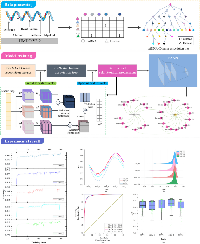
MicroRNAs (miRNAs) emerge in various organisms, ranging from viruses to humans, and play crucial regulatory roles within cells, participating in a variety of biological processes. In numerous prediction methods for miRNA-disease associations, the issue of over-dependence on both similarity measurement data and the association matrix still hasn’t been improved. In this paper, a miRNA-Disease association prediction model (called TP-MDA) based on tree path global feature extraction and fully connected artificial neural network (FANN) with multi-head self-attention mechanism is proposed. The TP-MDA model utilizes an association tree structure to represent the data relationships, multi-head self-attention mechanism for extracting feature vectors, and fully connected artificial neural network with 5-fold cross-validation for model training.

The experimental results indicate that the TP-MDA model outperforms the other comparative models, AUC is 0.9714. In the case studies of miRNAs associated with colorectal cancer and lung cancer, among the top 15 miRNAs predicted by the model, 12 in colorectal cancer and 15 in lung cancer were validated respectively, the accuracy is as high as 0.9227.

Conclusions

The model proposed in this paper can accurately predict the miRNA-disease association, and can serve as a valuable reference for data mining and association prediction in the fields of life sciences, biology, and disease genetics, among others.

Graphical Abstract

Peer Review reports

Introduction

MicroRNA (miRNA) is a class of short 20–24 nucleotide non-coding RNA molecules that play critical regulatory roles in cells [ 1 , 2 ]. They form a complex regulatory network and are involved in various biological processes such as cell proliferation, differentiation and apoptosis [ 3 ]. In addition, miRNA is closely related to the occurrence and development of cancer, cardiovascular diseases, nervous system diseases and other diseases [ 4 , 5 , 6 , 7 ]. For example, cancer stem cell-like cells (CSCs) are increasingly recognized as key cell tumor populations that drive not only tumorigenesis, but also cancer progression, treatment resistance, and metastatic recurrence. Existing evidence suggests that different metabolic pathways regulated by let-7 miRNA can impact CSC self-renewal, differentiation, and treatment resistance [ 8 ]. Therefore, in-depth research on the association between miRNAs and diseases is of great importance for understanding cellular regulatory mechanisms, discovering new therapeutic targets, and developing relevant biomedical applications [ 9 , 10 , 11 , 12 ].

With the continuous advancement of bioinformatics and the advent of the artificial intelligence era, researchers are increasingly using machine learning and deep learning algorithms to predict miRNA-disease associations [ 13 , 14 , 15 ]. It can provide validation guidance for biological experiments, thereby conserving resources and further advancing the field of miRNA and disease association prediction [ 16 , 17 , 18 ].It also has the potential to drive further advances in miRNA-disease association prediction. Based on different prediction strategies, existing methods can be categorized into four types: machine learning-based methods, information propagation-based methods, scoring function-based methods, and matrix transformation-based methods [ 19 , 20 ]. Machine learning-based prediction methods have recently become a focus and are gaining popularity among researchers [ 21 , 22 ]. Yu et al. [ 23 ] constructed a heterogeneous information network including miRNA, diseases, and genes. They defined seven symmetric meta-paths based on different semantic interpretations. After initializing the feature vectors for all nodes, they extracted and aggregated the vector information carried by all nodes on meta-path instances and updated the starting node’s feature vector. Then, they aggregated the vector information obtained from nodes on different meta-paths. Finally, they used miRNA and disease embedding feature vectors to compute their association scores. Xie et al. [ 24 ] constructed miRNA-disease bias scores using aggregated hierarchical clustering. A bipartite network recommendation algorithm was then used to assign transfer weights based on these bias ratings to predict potential miRNA-disease associations. Chen et al. [ 25 ] combined known miRNA and disease similarities to establish transfer weights and appropriately configured initial information. They then used a two-stage bipartite network algorithm to infer potential miRNA-disease associations.

In the study of miRNA-disease associations, there are two areas that need improvement: (1) The ability to capture indirect association features is inadequate. Among various computational methods, researchers use miRNA-disease heterogeneous networks to structure miRNA-disease association data and then extract feature vectors from the heterogeneous network. However, the associations within the heterogeneous network are limited to direct relationships between miRNAs and diseases, and their ability to capture indirect associations is often weak. This limitation may result in reduced model performance. (2) Over-reliance on similarity measurement data. Many computational methods rely on similarity information such as miRNA similarity and disease similarity for model training. The reliance on similarity data can, to a certain extent, influence the discriminative ability of the model and have an impact on its predictive accuracy.

To address the first issue, this paper investigates a data organization approach based on a tree-like topological structure. It represents miRNAs or diseases as root nodes and then searches for all related diseases or miRNAs as the second layer of the tree. All miRNAs or disease nodes associated with each disease or miRNA in the second layer are then found in the dataset. This process is repeated until the entire dataset has been thoroughly searched. At this point, there is a unique tree with the miRNA or disease as the root node, called the miRNA-disease association tree. This tree contains all association relationships related to that miRNA or disease within the dataset. Next, the vector information carried by all nodes on each path instance is extracted on the paths of the tree. Vector information obtained from nodes on different tree-paths is aggregated to generate feature vectors for model training. The miRNA-disease association tree has the potential to improve the capture of indirect association features. In response to Problem 2, since the similarity of data is often subjective based on some human-set metric, these data may produce misleading results in some cases, which in turn affects the performance of the algorithm. In contrast to similarity measures, multi-head self-attention mechanisms better capture long-distance dependencies in input sequences by allowing the model to focus on information from different locations, which in turn improves the predictive performance of the model. In this paper, we explore the use of the multi-head self-attention mechanism to fully extract the long dependencies carried by association trees, avoiding the bias created by using similarity measures and overcoming the problem of over-reliance on similarity measure data. As a result, the paper introduces a miRNA-disease association prediction model. This model uses a multi-head self-attention mechanism for comprehensive feature extraction on the tree-paths. It then trains the dataset using the Fully Connected Artificial Neural Network (FANN) model in a 5-fold cross-validation experiment. This model is referred to as TP-MDA.

Materials and methods

Establishing the association matrix.

Based on the miRNA-disease association information, remove duplicate, missing, and invalid data in order to construct the miRNA-disease association matrix. Given m miRNAs, M={m 1 、…、m i 、…、m m },and n diseases, D = {d 1 , …, d j , …, d n },the miRNA-disease association matrix is defined as R, where R ∈ R m×n , as shown in Eq. ( 1 ):

Subsequently, the miRNA-disease association tree is constructed by continuously exploring the association matrix. The process of association tree construction is shown in Fig.  1 .

The construction of the association tree

• Multi-head self-attention mechanism

The self-attention mechanism is a special type of attention mechanism used to handle relationships between different positions in sequence data. The multi-head self-attention mechanism is a common extension of the attention mechanism in deep learning that employs multiple attention heads at the same level, allowing for the fusion of different attention weights. In this paper, a multi-head self-attention mechanism is used to process the feature vectors extracted from the miRNA-disease association tree. The self-attention mechanism is as shown in Eqs. ( 2 ) and ( 3 ):

In the equations, X represents the vector information extracted from the miRNA-disease association tree, and Q, K, V represent the query matrix, key matrix, and value matrix, respectively. These three matrices are obtained by linear transformations of X using W Q , W K , and W V . Here, d k represents the dimension of the query, key, or value.

The multi-head self-attention mechanism transforms the linear matrices from a set ( \({\varvec{W}}^{\varvec{Q}},\) \({\varvec{W}}^{\varvec{K}},\) \({\varvec{W}}^{\varvec{V}}\) ) to multiple sets {( \({\varvec{W}}_{0}^{\varvec{Q}}\) , \({\varvec{W}}_{0}^{\varvec{K}}\) , \({\varvec{W}}_{0}^{\varvec{V}}\) ), …, ( \({\varvec{W}}_{\varvec{i}}^{\varvec{Q}}\) , \({\varvec{W}}_{\varvec{i}}^{\varvec{K}}\) , \({\varvec{W}}_{\varvec{i}}^{\varvec{V}}\) ) }. Different sets of linear matrices with random initialization ( \({\varvec{W}}^{\varvec{Q}}\) , \({\varvec{W}}^{\varvec{K}}\) , \({\varvec{W}}^{\varvec{V}}\) ) can map the input vectors to different subspaces, allowing the model to understand input information from different spatial dimensions. The multi-head attention mechanism is represented as shown in Eqs. ( 4 ) and ( 5 ):

In these equations, \({\varvec{W}}_{\varvec{i}}^{\varvec{Q}}\) , \({\varvec{W}}_{\varvec{i}}^{\varvec{K}}\) , \({\varvec{W}}_{\varvec{i}}^{\varvec{V}}\) represent the query matrix, key matrix, and value matrix for the i-th head, where h is the number of heads. \({\varvec{W}}^{\varvec{O}}\) is the linear transformation matrix used to map the output of the multi-head self-attention mechanism into the same dimensional space.

The key point of the self-attention mechanism is the ability to consider information about all other elements in the sequence while calculating the association between each element, rather than considering only a fixed number of adjacent elements as in traditional fixed window or convolution operations. Therefore, the self-attention mechanism can effectively manage long dependencies, allowing for improved capture of semantic information within the sequence, and there are numerous long dependencies to be addressed within the miRNA-disease association tree. In this paper, after the initial feature vector information is extracted from the tree nodes, the multi-head self-attention mechanism is used for information processing, resulting in the acquisition of the updated feature vector, which is used as input for model training. The operation principle is shown in Fig.  2 .

TP-MDA model

In the TP-MDA model, the miRNA-disease association matrix is transformed into a miRNA-disease association tree to explore long dependencies between nodes. A multi-head self-attention mechanism network is used to aggregate and extract information along the tree-paths. The outputs are concatenated to create feature vectors, which are subsequently used as input for training the FANN model. The schematic diagram of the TP-MDA model is illustrated in Fig.  3 .

Model diagram

In this paper, a Fully Connected Artificial Neural Network (FANN) is used to train the data. In addition to the input and output layers, three hidden layers have been configured. The ReLU (Rectified Linear Unit) function is used as the activation function, as depicted in Eq. ( 6 ):

For the output layer, a sigmoid function is set as the activation function, as shown in Eq. ( 7 ):

The loss function used is cross-entropy loss, and the TP-MDA model is trained using the Adam optimizer. The learning rate is set to 0.000001 and the number of iterations is set to 800. The prediction results of the model represent the predicted values for miRNA-disease associations.

Data source and model evaluation

The data in this paper is sourced from the Human microRNA Disease Database (HMDD, v4.0, http://www.cuilab.cn/hmdd ). The database is a widely used miRNA-disease association database that not only compiles experimentally validated miRNA-disease associations, but also enables normalized naming of miRNAs. The original dataset obtained from this database download contains 35,547 miRNA-disease association information. Since this data is a large dataset consisting of five assay methods, there are a certain number of duplicate entries. After removing duplicate entries and irrelevant information, the miRNA-disease association information is obtained, as shown in Table  1 .

As shown in Table  1 , a total of 21,152 miRNA-disease associations were obtained after preprocessing the dataset. A large sparse matrix with a dimension of 1207*889 was obtained from the construction of these data, and the miRNA-disease association tree was subsequently constructed by traversal operations on the matrix. During the training process of the TP-MDA model, samples with the same number of positive samples were randomly selected as negative samples among all unknown samples. In order to increase the generalization ability of the TP-MDA model to different sets of negative samples, it is set in the subsequent 5-fold cross-validation experiments that the negative samples selected in each experiment are not duplicated with the previous fold experiment.

During model training, a 5-fold cross-validation is used for training and validation, as shown in Eq. ( 8 ):

In the equation, k = 5 indicates the use of 5-fold cross-validation in the experiment, and MSE represents Mean Squared Error, a common measure used to evaluate the model’s performance.

When plotting the Receiver Operating Characteristic (ROC) curve, the data includes one-fifth of the positive samples and an equal number of randomly selected negative samples for validation. The true positive rate (TPR) and false positive rate (FPR) are calculated using the prediction results from this data, as shown in Eqs. ( 9 ) and ( 10 ):

In the equations, TP represents the number of correctly identified positive samples, while FN represents the number of incorrectly identified positive samples.

Where FP represents the number of incorrectly identified negative samples, and TN represents the number of correctly identified negative samples. By setting different classification thresholds, FPR and TPR are represented on the horizontal and vertical axes to create the Receiver Operating Characteristic (ROC) curve, which serves as one of the performance evaluation metrics for the model. The area under the ROC curve, defined as AUC, is typically considered an indicator of classifier performance, with larger AUC values associated with better classifier performance.

Additionally, accuracy is employed as one of the model evaluation metrics. In this paper, accuracy is calculated using validation data, as illustrated in Eq. ( 11 ):

The TP-MDA model consists of the following three parts: (1) Data processing: The miRNA-disease association data are transformed into an association matrix. The miRNA-disease association tree is constructed by continuously searching through the association matrix. In this paper, a miRNA-disease association tree is defined, with separate trees constructed using miRNA and disease as root nodes. All diseases or miRNAs associated with them in the association matrix are considered as the next-layer child nodes. Each disease or miRNA node is then traversed to identify its associated miRNAs or diseases. This process is repeated until the entire dataset has been completely traversed, yielding a distinct association tree with the miRNA or disease as the root node. (2) Feature Extraction: In the association tree, there are many long dependencies. The multi-head attention mechanism is employed to extract information held by the nodes of the tree structure. The information from different types of root nodes in the association tree is extracted separately and then concatenated to form feature vectors for potential miRNA-disease association prediction models. (3) Model training: The feature vectors are fed into a five-layer fully connected neural network whose output represents the miRNA-disease association score.

Analysis of node number optimization experiment results

In this paper, the data is trained using a 5-layer fully connected neural network, and the number of neurons in each fully connected layer is a critical parameter, especially in the last fully connected layer. The number of neurons in the final fully connected layer determines the dimension of the potential miRNA-disease interaction vectors, and this is a critical factor in predicting miRNA-disease associations [ 26 ]. However, running experiments with different hyperparameter combinations using LOOCV can be time-consuming. To save experimental resources, we only compare the performance of different numbers of neurons in the last fully connected layer. Therefore, we select different numbers of nodes for optimization with the goal of obtaining better parameters for model training. The AUC values of the model under different numbers of nodes are shown in Fig.  4 .

AUC statistical results of 800 rounds of experiments with different number of nodes. a AUC statistics when the number of nodes is 32, b AUC statistics when the number of nodes is 64, c AUC statistics when the number of nodes is 128, d AUC statistics when the number of nodes is 256

In the ridge plot, each peak represents one fold of the experiment, and it summarizes the AUC values during the 800 training rounds. The higher the peak, the more training rounds the model has reached at that specific AUC value, and peaks located to the right indicate a larger median in the statistical data, which corresponds to better model performance. As the number of nodes increases, the statistical results of the AUC value under the 5-fold cross-validation experiment are basically the same. The experimental results show that the best performance is observed in the fourth fold, while the second fold shows the worst performance. The median of all peaks is above 0.95, and in the fourth replicate there are more AUC values reaching 0.96. The results indicate that the HMDD v3.2 dataset can be effectively used for stable predictions in the TP-MDA model, which shows promising predictive performance in miRNA-disease association experiments. This suggests that the TP-MDA algorithm has superior performance in predicting miRNA-disease associations.

The experimental results for different numbers of nodes are statistically analyzed. A more detailed examination of all the results from the fourth fold in Fig.  4 is performed to determine the optimal number of nodes. The statistical results are shown in Fig.  5 .

The final experimental results under different nodes. a The final AUC experimental results under different number of nodes, b The final AUC statistics under different node numbers

The trend of AUC values remains consistent as the number of nodes changes in Fig.  5 a. When the number of nodes is set to 128, the AUC performance is superior to that at other node counts and is optimal in the second, third, and fourth fold experiments. The models with 32 and 128 nodes perform similarly in Fig.  5 b. By analyzing Fig.  5 a and b together, it can be concluded that the model performs better when the number of nodes is 128.

Analysis of learning rate optimization experiment results

The learning rate is crucial for determining whether the network model can converge to the optimal point, so a learning rate optimization process is carried out. The results are shown in Fig.  6 .

Experimental results at different learning rates. a When the learning rate is equal to 0.00001, the AUC statistical result of 800 rounds of experiments, b The final experimental results of AUC under different learning rates

During the learning rate optimization process, other parameters were held constant while the learning rate was changed. When the learning rate was set to 0.000001, it produced the same results as the model experiments shown in Fig.  4 d. In the experimental results shown in Fig.  4 d, there were no model AUC values that exceeded 0.97. In the experimental results shown in Fig.  6 a, some of the AUC values exceeded 0.97, at which point the learning rate (lr) was set to 0.00001. This indicates that when the learning rate is set to 0.00001, the model’s predictive performance improved over multiple rounds of experiments. Figure  6 b compares the final AUC values of the model under different learning rates, and the results show that the AUC values are consistently higher when lr = 0.00001 in the 5-fold cross-validation experiments compared to when lr = 0.000001. By optimizing the learning rate under the same experimental conditions, it was found that the prediction performance of the model is better when lr = 0.00001. The learning rate is crucial for TP-MDA to find the optimal point, and a more suitable learning rate parameter can improve the accuracy of miRNA-disease association prediction.

Comparison between association tree and association matrix in experiments

To validate whether the improvement of the miRNA-disease association tree has a positive impact on the model, this paper conducted experiments with the same experimental parameters on the miRNA-disease association matrix. In these experiments, the rows and columns of the association matrix were concatenated to form a vector. Attention mechanisms were then used to extract feature vectors, and the resulting vectors were fed into a fully connected neural network for training. A comparison of the model training results using the miRNA-disease association matrix and the miRNA-disease association tree as inputs is shown in Fig.  7 .

Comparison of AUC values of association matrix and association tree. a Comparison of AUC results under 5-fold cross-validation experiment using association matrix and association tree as input, b Statistics of AUC results under 5-fold cross-validation experiment using association matrix and association tree as input

The green line represents the AUC results obtained using the miRNA-disease association tree as input, while the yellow line represents the AUC results obtained using the miRNA-disease association matrix as input, as shown in Fig.  7 a. In the experiments with 5-fold cross-validation using the association tree as input, the AUC values exceeded 0.97, while using the association matrix as input did not reach 0.94. The model using the miRNA-disease association tree shows significantly better and more stable performance under 5-fold cross-validation, as shown in Fig.  7 b. The experimental results show a significant improvement in predictive performance when using the association tree as input, indicating the superiority of the TP-MDA model in predicting potential miRNA-disease associations.

Comparing the model experimental results using accuracy as the evaluation parameter for models with association matrix and association tree as inputs, the results are shown in Figs.  8 and 9 .

Accuracy statistics of model prediction results using miRNA-disease association matrix as input were obtained in the 5-fold cross-validation experiment, and 800 rounds of model training were performed in each fold experiment

Comparison of accuracy results under 5-fold cross-validation experiment using association matrix and association tree as input

When training the model using the miRNA-disease association matrix as input, the accuracy remains below 0.9 in all cases, as shown in Fig.  8 . The blue line in Fig.  9 represents the model trained with the association tree as input. In four out of five folds, the accuracy is better than 0.9, and all of them outperform the results obtained with the association matrix as input. This shows a significant improvement in accuracy. It can be concluded that by using the miRNA-disease association tree as input, a more reliable prediction model can be obtained, which can more accurately predict the potential miRNA-disease association.

Analysis of experiments with the optimal model parameters

The TP-MDA model is trained with the optimal parameters under 5-fold cross-validation. ROC curves are plotted on the basis of the prediction results and the experimental results are statistically analyzed, as shown in Fig.  10 .

AUC experiment results of optimal parameters. a When the optimal parameters are used, the ROC curve under the experiment is 5-fold cross-verified, b Statistics of AUC results of TP-MDA model in 800 rounds of experiments

The lowest AUC value in Fig.  10 a reaches 0.9691 in the 5-fold cross-validation experiments. The statistical results in Fig.  10 b show that more than 50% of the AUC values are greater than 0.97, indicating that this set of experimental parameters performs well during model training, leading to an improvement in the predictive performance of the model. At the same time, the model exhibits considerable stability across the entire dataset, avoiding the randomness of good model performance due to unbalanced sample selection. Compared to using the miRNA-disease association matrix as the model input, extracting the numerous node relationships from the association tree as feature vectors can result in a more accurate and superior prediction model for miRNA-disease associations.

Accuracy, as another parameter to evaluate, is critical to improving model performance. The changes in accuracy as the model is trained with optimal parameters are shown in Figs.  11 and 12 .

The accuracy statistics of the model were obtained by using the optimal parameters and the miRNA-disease association tree as input

The accuracy distribution of the model was obtained by using the optimal parameters and the miRNA-disease association tree as input

There is a fluctuation in accuracy in each fold of the experiment, but the overall trend is upward and stabilizes around 600 training cycles, as shown in Fig.  11 . The selection of these models for further training can have more reliable prediction results. The accuracy distribution of the 800 training cycles in a 5-fold cross-validation experiment is shown in Fig.  12 . The highest accuracy is 0.9227. More than 50% of the data in the four folds exceed 0.9. The experimental results show that the model performs better when the parameters are optimized. This also confirms the stability and efficiency of the TP-MDA model.

Comparison and analysis with other models

In this paper, TP-MDA was compared to three other miRNA-based models for predicting disease association using 5-fold cross validation. Comparison models are shown in Table  2 .

The comparison of the AUC results for the four different models is shown in Fig.  13 .

Graph comparing AUC values with other models

TP-MDA obtained the highest AUC value. WBNPMD and BNPMDA had lower AUC values because they predicted miRNA-disease associations by resource allocation and transfer, which over-relied on the similarity matrix and affected their predictive performance. Compared to these two models, MDPBMP used 0.5 as the threshold to filter miRNA similarity, improved the reliability of similarity values, and increased the prediction accuracy by constructing feature vectors for nodes and aggregating information from all nodes in each meta path instance. The TP-MDA model presented in this paper does not rely on any known similarity measures. Instead, it uses the construction of a miRNA-disease association tree to describe the global relationships between nodes. It uses an efficient model to learn long dependencies within the association tree, resulting in a high-performing model with the highest AUC value.

Case studies

For our case studies, we chose colorectal cancer [ 27 , 28 , 29 , 30 ] and lung cancer [ 31 , 32 ], two common cancers. We used TP-MDA to score and rank the relevance of miRNA for unknown samples. The top 15 miRNAs were selected for validation by comparison with biomedical literature from the PubMed database. The predicted results of miRNA associated with colorectal cancer are shown in Table  3 .

The validation results for lung cancer based on the predictions of the TP-MDA model are shown in Table  3 . In the miRNA naming convention, “-1” and “-2” are added to the miRNA names to indicate that these miRNAs are transcribed and processed from DNA sequences on different chromosomes but share the same mature sequence [ 45 ]. Therefore, even though the top-ranked miRNA, hsa-mir-101-2, hasn’t been directly validated to be associated with colorectal cancer, it is known that miRNA hsa-mir-101, which shares the same mature sequence, is associated with colorectal cancer. Therefore, there is an association between the miRNA hsa-mir-101-2 and colorectal cancer. In summary, of the top 15 miRNAs predicted to be associated with colorectal cancer by TP-MDA, 12 were validated.

The prediction results of miRNA associated with lung cancer are shown in Table  4 :

The top 15 miRNAs predicted to be associated with lung cancer by the TP-MDA model are shown in Table  4 . Among them, the sixth ranked miRNA, hsa-mir-30b, and the tenth ranked miRNA, hsa-mir-30b, share a high degree of sequence homology. The eleventh ranked miRNA, hsa-let-7c, follows an earlier nomenclature and is primarily used to represent the let-7 miRNA family. The study by Yin et al. [ 60 ] demonstrated that the let-7 miRNA family is involved in the regulation of resistance to epidermal growth factor receptor tyrosine kinase inhibitors (EGFR-TKIs) and may serve as predictive biomarker for EGFR-TKI resistance in non-small cell lung cancer (NSCLC). EGFR-TKI resistance represents a significant challenge in treating NSCLC. In summary, all of the top 15 miRNAs predicted to be associated with lung cancer by TP-MDA were validated. The statistics and visualization of the verification results are shown in Fig.  14 .

Case study results statistics and visualization. a The proportion of the number of results obtained by actual verification, b Number of validation results, c Validation result visualization

Among the top 15 miRNAs associated with colorectal cancer and lung cancer, 12 and 15 miRNAs were validated, accounting for 80% and 100% of the total validated miRNAs, respectively, as shown in Fig.  12 a and b. Among the top 15 predicted miRNAs associated with colorectal cancer and lung cancer, hsa-mir-219 is associated with both diseases simultaneously, as shown in Fig.  14 c. The miRNA hsa-mir-181a-1, which is associated with colorectal cancer, shares the same mature sequence with hsa-mir-181a, which is associated with lung cancer. In addition, the hsa-let-7 family members, hsa-let-7f and hsa-let-7c, are associated with colorectal cancer and lung cancer, respectively. This suggests that the relationships between miRNAs and diseases are complex and that the TP-MDA model has the ability to predict complex associations between miRNAs and diseases.

This paper introduces the TP-MDA miRNA-disease association prediction model. This model does not rely on any similarity measures and employs a multi-head self-attention mechanism to extract global vector information from the miRNA-disease association tree. Finally, the model is trained using a FANN framework in a 5-fold cross-validation experiment. The experimental results show that this algorithm performs excellently in predicting miRNA-disease associations. It shows good and stable performance in cross-validation. Compared with other models, it has better prediction effect. The TP-MDA model can serve as a reference method for data mining and association prediction in various fields, including life sciences, biology, and medical genetics. However, the field of miRNA-disease association prediction still needs to be further explored despite the positive experimental results. For example, understanding the complex interactions between different biological information in disease mechanisms is a significant challenge. In future work, the development of algorithms capable of handling multiple types of biological information will be critical to achieving more accurate and effective predictions in this area.

Availability of data and materials

The codes, architecture, parameters, dataset, functions, usage and output of the proposed model are available free of charge at GitHub. ( https://github.com/BiyuHou/miRNA-disease.git ).

Wu L, et al. Research progress on plant long non-coding RNA. Plants (Basel). 2020;9(4):408.

CAS   PubMed   Google Scholar  

Wang S, et al. Computational annotation of miRNA transcription start sites. Brief Bioinform. 2021;22(1):380–92.

Article   PubMed   Google Scholar  

Darbeheshti F, et al. Investigation of BRCAness associated miRNA-gene axes in breast cancer: cell-free mir-182-5p as a potential expression signature of BRCAness. BMC Cancer. 2022;22(1):668.

Article   PubMed   PubMed Central   Google Scholar  

Toden S, Zumwalt TJ, Goel A. Non-coding RNAs and potential therapeutic targeting in cancer. Biochim Biophys Acta Rev Cancer. 2021;1875(1):188491.

Article   CAS   PubMed   Google Scholar  

Pan L, et al. Association between single nucleotide polymorphisms of miRNAs and gastric cancer: a scoping review. Genet Test Mol Biomarkers. 2022;26(10):459–67.

Park JH, et al. Genetic variations in MicroRNA genes and cancer risk: a field synopsis and meta-analysis. Eur J Clin Invest. 2020;50(4):e13203.

Son SM, et al. MicroRNA 29a therapy for CEACAM6-expressing lung adenocarcinoma. BMC Cancer. 2023;23(1):843.

Article   CAS   PubMed   PubMed Central   Google Scholar  

Ma Y, et al. The roles of the Let-7 family of MicroRNAs in the regulation of cancer stemness. Cells. 2021;10(9):2415.

Arfin S, et al. Differentially expressed genes, miRNAs and network models: a strategy to shed light on molecular interactions driving HNSCC tumorigenesis. Cancers (Basel). 2023;15(17):4420.

Jabeer A, et al. miRdisNET: discovering microRNA biomarkers that are associated with diseases utilizing biological knowledge-based machine learning. Front Genet. 2022;13:1076554.

Simiene J, et al. Potential of miR-181a-5p and miR-630 as clinical biomarkers in NSCLC. BMC Cancer. 2023;23(1):857.

Wang Z, et al. MiR-16-5p suppresses breast cancer proliferation by targeting ANLN. BMC Cancer. 2021;21(1):1188.

Liu B, et al. Combined embedding model for MiRNA-disease association prediction. BMC Bioinformatics. 2021;22(1):161.

Lou Z, et al. Predicting miRNA-disease associations via learning multimodal networks and fusing mixed neighborhood information. Brief Bioinform. 2022;23(5):bbac159.

Wang XF, et al. KS-CMI: a circRNA-miRNA interaction prediction method based on the signed graph neural network and denoising autoencoder. iScience. 2023;26(8):107478.

Jing R, et al. layerUMAP: a tool for visualizing and understanding deep learning models in biological sequence classification using UMAP. iScience. 2022;25(12):105530.

Yousef M, et al. miRcorrNet: machine learning-based integration of miRNA and mRNA expression profiles, combined with feature grouping and ranking. PeerJ. 2021;9:e11458.

Cao B, et al. Predicting miRNA-disease association through combining miRNA function and network topological similarities based on MINE. iScience. 2022;25(11):105299.

Yu L, et al. Research progress of miRNA-disease association prediction and comparison of related algorithms. Brief Bioinform. 2022;23(3):bbac066.

Gu C, Li X. Prediction of disease-related miRNAs by voting with multiple classifiers. BMC Bioinformatics. 2023;24(1):177.

Ji BY, et al. Predicting miRNA-disease association from heterogeneous information network with GraRep embedding model. Sci Rep. 2020;10(1):6658.

Ghobadi MZ, Emamzadeh R, Afsaneh E. Exploration of mRNAs and miRNA classifiers for various ATLL cancer subtypes using machine learning. BMC Cancer. 2022;22(1):433.

Yu L, Zheng Y, Gao L. MiRNA-disease association prediction based on meta-paths. Brief Bioinform. 2022;23(2):bbab571.

Xie G, et al. WBNPMD: weighted bipartite network projection for microRNA-disease association prediction. J Transl Med. 2019;17(1):322.

Chen X, et al. BNPMDA: bipartite network projection for MiRNA-disease association prediction. Bioinformatics. 2018;34(18):3178–86.

Zeng M, et al. DMFLDA: a deep learning framework for predicting lncRNA-disease associations. IEEE/ACM Trans Comput Biol Bioinform. 2021;18(6):2353–63.

Itakura H, et al. Tumor-suppressive role of the musculoaponeurotic fibrosarcoma gene in colorectal cancer. iScience. 2023;26(4):106478.

Chiu CC, et al. Correlation of body mass index with oncologic outcomes in colorectal cancer patients: a large population-based study. Cancers (Basel). 2021;13(14):3592.

Ullah I, et al. Multi-omics approaches in colorectal cancer screening and diagnosis, recent updates and future perspectives. Cancers (Basel). 2022;14(22):5545.

Heublein S, et al. Association of differential miRNA expression with hepatic vs. peritoneal metastatic spread in colorectal cancer. BMC Cancer. 2018;18(1):201.

Gencel-Augusto J, Wu W, Bivona TG. Long non-coding RNAs as emerging targets in lung cancer. Cancers (Basel). 2023;15(12):3135.

Shao C, et al. The value of miR-155 as a biomarker for the diagnosis and prognosis of lung cancer: a systematic review with meta-analysis. BMC Cancer. 2019;19(1):1103.

Wang XW, et al. SIRT1 promotes the progression and chemoresistance of colorectal cancer through the p53/miR-101/KPNA3 axis. Cancer Biol Ther. 2023;24(1):2235770.

Javanmard AR, et al. LOC646329 long non-coding RNA sponges miR-29b-1 and regulates TGFβ signaling in colorectal cancer. J Cancer Res Clin Oncol. 2020;146(5):1205–15.

Pliakou E, et al. Circulating miRNA expression profiles and machine learning models in association with response to irinotecan-based treatment in metastatic colorectal cancer. Int J Mol Sci. 2022;24(1):46.

Han C, Song Y, Lian C. MiR-769 inhibits colorectal cancer cell proliferation and invasion by targeting HEY1. Med Sci Monit. 2018;24:9232–9.

Bjeije H, et al. YWHAE long non-coding RNA competes with miR-323a-3p and mir-532-5p through activating K-Ras/Erk1/2 and PI3K/Akt signaling pathways in HCT116 cells. Hum Mol Genet. 2019;28(19):3219–31.

Gu J, et al. Astragalus mongholicus Bunge-Curcuma aromatica Salisb. suppresses growth and metastasis of colorectal cancer cells by inhibiting M2 macrophage polarization via a Sp1/ZFAS1/miR-153-3p/CCR1 regulatory axis. Cell Biol Toxicol. 2022;38(4):679–97.

Xu H, et al. CircRNA_0000392 promotes colorectal cancer progression through the miR-193a-5p/PIK3R3/AKT axis. J Exp Clin Cancer Res. 2020;39(1):283.

Chen LY, et al. The circular RNA circ-ERBIN promotes growth and metastasis of colorectal cancer by miR-125a-5p and miR-138-5p/4EBP-1 mediated cap-independent HIF-1α translation. Mol Cancer. 2020;19(1):164.

Niculae AM, et al. Let-7 microRNAs are possibly associated with perineural invasion in colorectal cancer by targeting IGF axis. Life (Basel). 2022;12(10):1638.

Tang HQ, et al. Decreased long noncoding RNA ADIPOQ promoted cell proliferation and metastasis via miR-219c-3p/TP53 pathway in colorectal carcinoma. Eur Rev Med Pharmacol Sci. 2020;24(14):7645–54.

PubMed   Google Scholar  

Wang N, et al. Serum miR-663 expression and the diagnostic value in colorectal cancer. Artif Cells Nanomed Biotechnol. 2019;47(1):2650–3.

Yang K, et al. Rosmarinic acid inhibits migration, invasion, and p38/AP-1 signaling via mir-1225-5p in colorectal cancer cells. J Recept Signal Transduct Res. 2021;41(3):284–93.

Budak H, et al. MicroRNA nomenclature and the need for a revised naming prescription. Brief Funct Genomics. 2016;15(1):65–71.

Chen Y, et al. MiR-181a reduces radiosensitivity of non-small-cell lung cancer via inhibiting PTEN. Panminerva Med. 2022;64(3):374–83.

Ma J, Qi G, Li L. LncRNA NNT-AS1 promotes lung squamous cell carcinoma progression by regulating the miR-22/FOXM1 axis. Cell Mol Biol Lett. 2020;25:34.

Pirlog R, et al. Cellular and molecular profiling of tumor microenvironment and early-stage lung cancer. Int J Mol Sci. 2022;23(10):5346.

Qu CX, et al. LncRNA CASC19 promotes the proliferation, migration and invasion of non-small cell lung carcinoma via regulating miRNA-130b-3p. Eur Rev Med Pharmacol Sci. 2019;23(3 Suppl):247–55.

Charkiewicz R, et al. miRNA-Seq tissue diagnostic signature: a novel model for NSCLC subtyping. Int J Mol Sci. 2023;24(17):13318.

Shangguan WJ, et al. TOB1-AS1 suppresses non-small cell lung cancer cell migration and invasion through a ceRNA network. Exp Ther Med. 2019;18(6):4249–58.

CAS   PubMed   PubMed Central   Google Scholar  

Shen Q, Sun Y, Xu S. LINC01503/miR-342-3p facilitates malignancy in non-small-cell lung cancer cells via regulating LASP1. Respir Res. 2020;21(1):235.

Sun SN, et al. Relevance function of microRNA-708 in the pathogenesis of cancer. Cell Signal. 2019;63:109390.

Young MJ, et al. Estradiol-mediated inhibition of Sp1 decreases miR-3194-5p expression to enhance CD44 expression during lung cancer progression. J Biomed Sci. 2022;29(1):3.

Shadbad MA, et al. A scoping review on the significance of programmed death-ligand 1-inhibiting microRNAs in non-small cell lung treatment: a single-cell RNA sequencing-based study. Front Med (Lausanne). 2022;9:1027758.

Xie L, et al. SKA3, negatively regulated by miR-128-3p, promotes the progression of non-small-cell lung cancer. Per Med. 2022;19(3):193–205.

Peng XX, et al. Correlation of plasma exosomal microRNAs with the efficacy of immunotherapy in EGFR/ALK wild-type advanced non-small cell lung cancer. J Immunother Cancer. 2020;8(1):e000376.

Wang Q, et al. XB130, regulated by miR-203, miR-219, and miR-4782-3p, mediates the proliferation and metastasis of non-small-cell lung cancer cells. Mol Carcinog. 2020;59(5):557–68.

Yang S, et al. Expression of miR-486-5p and its significance in lung squamous cell carcinoma. J Cell Biochem. 2019;120(8):13912–23.

Yin J, et al. let–7 and miR–17 promote self–renewal and drive gefitinib resistance in non–small cell lung cancer. Oncol Rep. 2019;42(2):495–508.

Download references

The authors gratefully acknowledge the support from the National Natural Science Foundation of China 21(Grant Numbers: 51663001, 52063002, 42061067, 61741202).

Author information

Authors and affiliations.

College of Physics and Electronic Information, Gannan Normal University, Ganzhou, Jiangxi, 341000, China

Hou Biyu, Li Mengshan, Zeng Ming & Guan Lixin

College of Computer Science and Engineering, Shanxi Datong University, Datong, Shanxi, 037000, China

College of Life Sciences, Jiaying University, Meizhou, Guangdong, 514000, China

You can also search for this author in PubMed   Google Scholar

Contributions

Li Mengshan and Hou Biyu designed the study; Zeng Ming and Hou Yuxin performed the research; Li Mengshan and Hou Biyu conceived the idea; Guan Lixin and Wang Nan provided and analyzed the data; Zeng Ming and Hou Biyu helped perform the analysis with constructive discussions; all authors contributed to writing and revision. All authors read and approved the final manuscript.

Corresponding author

Correspondence to Li Mengshan .

Ethics declarations

Competing interests.

The authors declare no competing interests.

Conflict of interest

No potential conflict of interest was reported by authors.

Additional information

Publisher’s note.

Springer Nature remains neutral with regard to jurisdictional claims in published maps and institutional affiliations.

Rights and permissions

Open Access This article is licensed under a Creative Commons Attribution 4.0 International License, which permits use, sharing, adaptation, distribution and reproduction in any medium or format, as long as you give appropriate credit to the original author(s) and the source, provide a link to the Creative Commons licence, and indicate if changes were made. The images or other third party material in this article are included in the article's Creative Commons licence, unless indicated otherwise in a credit line to the material. If material is not included in the article's Creative Commons licence and your intended use is not permitted by statutory regulation or exceeds the permitted use, you will need to obtain permission directly from the copyright holder. To view a copy of this licence, visit http://creativecommons.org/licenses/by/4.0/ . The Creative Commons Public Domain Dedication waiver ( http://creativecommons.org/publicdomain/zero/1.0/ ) applies to the data made available in this article, unless otherwise stated in a credit line to the data.

Reprints and permissions

About this article

Cite this article.

Biyu, H., Mengshan, L., Yuxin, H. et al. A miRNA-disease association prediction model based on tree-path global feature extraction and fully connected artificial neural network with multi-head self-attention mechanism. BMC Cancer 24 , 683 (2024). https://doi.org/10.1186/s12885-024-12420-5

Download citation

Received : 18 November 2023

Accepted : 23 May 2024

Published : 05 June 2024

DOI : https://doi.org/10.1186/s12885-024-12420-5

Share this article

Anyone you share the following link with will be able to read this content:

Sorry, a shareable link is not currently available for this article.

Provided by the Springer Nature SharedIt content-sharing initiative

• Association tree
• miRNA-disease association
• Deep learning

ISSN: 1471-2407

• Submission enquiries: [email protected]
• General enquiries: [email protected]

Loading metrics

Open Access

Peer-reviewed

Research Article

Leveraging conformal prediction to annotate enzyme function space with limited false positives

Roles Data curation, Investigation, Methodology, Software, Validation, Visualization, Writing – original draft, Writing – review & editing

Affiliation School of Computational Science and Engineering, Georgia Institute of Technology, Atlanta, Georgia, United States of America

Roles Investigation, Methodology, Software, Writing – original draft, Writing – review & editing

Roles Conceptualization, Funding acquisition, Investigation, Methodology, Project administration, Resources, Supervision, Writing – original draft, Writing – review & editing

* E-mail: [email protected]

• Kerr Ding, 
• Jiaqi Luo, 

• Published: May 29, 2024
• https://doi.org/10.1371/journal.pcbi.1012135
• Reader Comments

This is an uncorrected proof.

Machine learning (ML) is increasingly being used to guide biological discovery in biomedicine such as prioritizing promising small molecules in drug discovery. In those applications, ML models are used to predict the properties of biological systems, and researchers use these predictions to prioritize candidates as new biological hypotheses for downstream experimental validations. However, when applied to unseen situations, these models can be overconfident and produce a large number of false positives. One solution to address this issue is to quantify the model’s prediction uncertainty and provide a set of hypotheses with a controlled false discovery rate (FDR) pre-specified by researchers. We propose CPEC, an ML framework for FDR-controlled biological discovery. We demonstrate its effectiveness using enzyme function annotation as a case study, simulating the discovery process of identifying the functions of less-characterized enzymes. CPEC integrates a deep learning model with a statistical tool known as conformal prediction, providing accurate and FDR-controlled function predictions for a given protein enzyme. Conformal prediction provides rigorous statistical guarantees to the predictive model and ensures that the expected FDR will not exceed a user-specified level with high probability. Evaluation experiments show that CPEC achieves reliable FDR control, better or comparable prediction performance at a lower FDR than existing methods, and accurate predictions for enzymes under-represented in the training data. We expect CPEC to be a useful tool for biological discovery applications where a high yield rate in validation experiments is desired but the experimental budget is limited.

Author summary

Machine learning (ML) models are increasingly being applied as predictors to generate biological hypotheses and guide biological discovery. However, when applied to unseen situations, ML models can be overconfident and make enormous false positive predictions, resulting in the challenges for researchers to trade-off between high yield rates and limited budgets. One solution is to quantify the model’s prediction uncertainty and generate predictions at a controlled false discovery rate (FDR) pre-specified by researchers. Here, we introduce CPEC, an ML framework designed for FDR-controlled biological discovery. Using enzyme function prediction as a case study, we simulate the process of function discovery for less-characterized enzymes. Leveraging a statistical framework, conformal prediction, CPEC provides rigorous statistical guarantees that the FDR of the model predictions will not surpass a user-specified level with high probability. Our results suggested that CPEC achieved reliable FDR control for enzymes under-represented in the training data. In the broader context of biological discovery applications, CPEC can be applied to generate high-confidence hypotheses and guide researchers to allocate experimental resources to the validation of hypotheses that are more likely to succeed.

Citation: Ding K, Luo J, Luo Y (2024) Leveraging conformal prediction to annotate enzyme function space with limited false positives. PLoS Comput Biol 20(5): e1012135. https://doi.org/10.1371/journal.pcbi.1012135

Editor: Cameron Mura, University of Virginia, UNITED STATES

Received: September 2, 2023; Accepted: May 3, 2024; Published: May 29, 2024

Copyright: © 2024 Ding et al. This is an open access article distributed under the terms of the Creative Commons Attribution License , which permits unrestricted use, distribution, and reproduction in any medium, provided the original author and source are credited.

Data Availability: The dataset underlying this article was derived from sources in the public domain. We used the data downloaded from https://github.com/flatironinstitute/DeepFRI . Our code is publicly available at https://github.com/luo-group/CPEC .

Funding: This work is supported in part by the National Institute Of General Medical Sciences of the National Institutes of Health ( https://www.nih.gov/ ) under the award R35GM150890, the 2022 Amazon Research Award ( https://www.amazon.science/research-awards ), and the Seed Grant Program from the NSF AI Institute: Molecule Maker Lab Institute (grant #2019897) at the University of Illinois Urbana-Champaign (UIUC; https://moleculemaker.org/ ). The funders had no role in study design, data collection and analysis, decision to publish, or preparation of the manuscript.

Competing interests: The authors have declared that no competing interests exist.

Introduction

Machine learning (ML) algorithms have proven to be transformative tools for generating biological hypotheses and uncovering knowledge from large datasets [ 1 , 2 ]. Applications include designing function-enhanced proteins [ 3 , 4 ], searching for novel drug molecules [ 5 ], and optimizing human antibodies against new viral variants [ 6 ]. These discoveries often involve a combination of computation and experimentation, where ML-based predictive models generate biological hypotheses and wet-lab experiments are then used to validate them. This approach is beneficial as it greatly reduces the search space and eliminates candidates that are unlikely to be successful, thus saving time and resources in the discovery process. For example, in drug discovery, ML has become a popular strategy for virtual screening of molecule libraries, where researchers use ML models to predict the properties of molecules, such as binding affinity to a target, and identify the most promising candidates for downstream experimental validation and lead optimization [ 7 ].

To gain new insights into biological systems or make novel discoveries (e.g., designing new drugs), ML algorithms are often used to make predictions for previously unseen data samples. For example, to support the design of new vaccines or therapeutics for COVID-19, ML algorithms need to predict the potential for immune escape of future variants that are composed of mutations that have not yet been seen. Similarly, in drug screening, ML algorithms should be able to predict molecules that are structurally different from those in the training data, which helps scientists avoid re-discovering existing drugs. However, making predictions for samples that are under-represented in the training data is a challenging task in ML. While human experts can assess the success likelihood of generated hypotheses based on their domain knowledge or intuition, this ability is not naturally developed by an ML model and, as a result, the model could be susceptible to pathological failure and only provide overconfident or unreliable predictions. This can have critical implications in ML-assisted biological discovery, as unreliable ML predictions can guide experimental efforts in the wrong direction, wasting resources on validating false positives.

In this work, we aim to develop ML models that can generate hypotheses with limited false positives, providing confident and accurate predictions that can potentially help improve the yield rate in downstream validation experiments. Specifically, we use the function annotation problem of protein enzymes as an example to demonstrate our method. The underlying computational problem of function annotation is a multi-class, multi-label classification problem as a protein can have multiple functions. In computational protein function annotation, a model typically predicts a set of functions that the query protein may potentially have. The set of predicted functions, if validated by experiments, can be incorporated into existing databases to augment our knowledge of the protein function space. There is often a trade-off regarding the size of the prediction set: researchers prefer a set with a small size, containing a handful of very confident predictions, as it is not desirable to spend resources on too many hypotheses that ultimately turn out to be false positives; on the other hand, researchers may be willing to increase the budget to validate a larger set of predictions in order to improve the chance of discovering novel functions for under-studied proteins.

The above tradeoff is often captured by different notions of prediction score cutoff, which decides whether to assign a particular function label to a protein, in existing computational methods for function annotation. For example, when annotating protein functions using sequence-similarity-based tools such as BLAST [ 8 ], a cutoff of the BLAST E-value can be used to determine the significance of sequence match. However, the choice of E-value cutoff is often based on the user’s intuition and good cutoff values on a dataset may not generalize to another dataset. Recent ML methods for enzyme function annotation typically first predict the probability that the input protein has a particular function and annotate the protein with this function if the predicted probability is greater than 0.5 [ 9 – 11 ]. However, using an arbitrary cutoff such as 0.5 is problematic as the predicted probabilities do not always translate to the confidence of the ML model, especially when the model is not well-calibrated (e.g., a predicted function with probability 0.95 may still be an unreliable prediction if the model is overconfident and produces very high probability scores most of the time). Recently, Hie et al. [ 12 ] developed a framework that used the Gaussian process to estimate the confidence or uncertainty in the ML model’s predictions. While the framework was shown to be effective to guide biological discovery, it is unclear how the estimated uncertainty is related to the final false discovery rate (FDR) in experimental validation and how to set a cutoff on the uncertainty scores to achieve a desired FDR. Consequently, it is challenging to provide FDR estimates before the experimental validation, and FDR typically can only be assessed post-validation.

Here, we propose an ML method, called CPEC (Conformal Prediction of EC number), to achieve FDR-controlled enzyme function prediction by leveraging a statistical framework known as conformal prediction (CP) [ 13 ]. CPEC receives the sequence or structure of an enzyme as input and predicts a set of functions (EC numbers) that the enzyme potentially has. The unique strength of CPEC is that the averaged per-protein FDR (i.e., the number of incorrect predictions divided by the prediction set size for a protein) can be controlled by a user-specified hyper-parameter α . The CP framework theoretically guarantees that the FDR of our per-protein predictions is no larger than α with a very high probability. This equips researchers with foresight, offering success rate estimates even before experimental validation. In an ML-guided workflow of protein function discovery, researchers can specify the desired FDR level α based on the experiment budget or expectations. For example, setting α to a smaller value when only the most confident predictions are needed or the test budget is limited, or setting to a larger value when the goal is to discover novel functions and a slightly higher FDR and budget are acceptable. The base ML model of CPEC is PenLight2, an improved version of the deep learning model PenLight [ 14 ] for the multi-class multi-label protein function annotation problem, which uses a graph neural network to integrate 3D protein structure data and protein language model embeddings to learn structure-aware representations for function prediction. Benchmarked on a carefully curated dataset, we first found that CPEC outperformed existing deep learning methods for enzyme function prediction. We also demonstrated that CPEC provides rigorous guarantees of FDR and allows users to trade-off between precision and recall in the predictions by tuning the desired maximum value α of FDR. Additionally, we showed that CPEC consistently provides FDR-controlled predictions for proteins with different sequence identities to the training set, suggesting its robustness even in regimes beyond its training data distribution. Moreover, based on CPEC, we proposed a cascade model that can better balance the resolution and coverage for EC number prediction.

Materials and methods

Problem formulation.

• PPT PowerPoint slide
• PNG larger image
• TIFF original image

(A) CPEC is a machine learning (ML) framework that leverages conformal prediction to control the false discovery rate (FDR) while performing enzyme function predictions. Compared to conventional ML predictions, CPEC allows users to select the desired FDR tolerance α and generates corresponding FDR-controlled prediction sets. Enabled by conformal prediction, CPEC provides a rigorous statistical guarantee such that the FDR of its predictions will not exceed the FDR tolerance α set by the users. The FDR tolerance α offers flexibilities in ML-guided biological discovery: when α is small, CPEC only produces hypotheses for which it has the most confidence; a larger α value would allow CPEC to afford a higher FDR, and CPEC thus can predict a set with more function labels to improve the true positive rate. Abbreviation: Func: function. Incorrect predictions in prediction sets are colored gray. (B) We developed a deep learning model, PenLight2, as the base model of the CPEC framework. The model is a graph neural network that receives the three-dimensional structure and the sequence of a protein as input and generates a function-aware representation for the protein. It employs a contrastive learning scheme to learn a vector representation for proteins, such that the representations of functionally similar proteins in the latent space are pulled together while dissimilar proteins are pushed apart.

https://doi.org/10.1371/journal.pcbi.1012135.g001

Conformal risk control

Overview of conformal risk control..

Conformal risk control guarantee for FDR control.

Calibration algorithm for FDR control.

Given the FDR control guarantee, the natural follow-up question would be how to find a valid parameter λ that can control the risk through the calibration step on calibration data. The Learn then Test (LTT) algorithm [ 22 ], which formulated the selection of λ as a multiple hypotheses testing problem, has been proposed to solve this question. CPEC adopts the LTT algorithm established upon the data distribution assumption that all feature-response pairs ( X , Y ) from the calibration set and the test set are independent and identically distributed (i.i.d.).

Algorithm 1: CPEC for FDR control

/* Calculation of Hoeffding’s inequality p-values { p 1 , …, p N }    */

for i ← 1 N do

  for j ← 1 n c do

while p i ≤ δ and i ≥ 1 do

  i ← i − 1;

Protein function prediction

Ec number prediction dataset..

We applied CPEC on the task of Enzyme Commission (EC) numbers [ 17 ] prediction to demonstrate its effectiveness. EC number is a widely used four-level classification scheme, which organizes the protein according to their functions of catalyzing biochemical reactions. In specific, a protein would be labeled with an EC number if it catalyzes the type of biochemical reactions represented by that EC number. For each four-digit EC number a . b . c . d , the 1st-level a is the most general classification level while the 4th-level d is the most specific one. We used the dataset that contains EC number-labeled protein sequences and structures, provided by Gligorijević et al. [ 10 ]. The protein structures were retrieved from Protein Data Bank (PDB) [ 27 ]. Protein chains were then clustered at 95% sequence identity using the BLASTClust function in the BLAST tool [ 8 ] and then organized into a non-redundant set which only included one labeled high-resolution protein chain from each cluster. The EC number annotations were collected from SIFTS (structure integration with function, taxonomy, and sequence) [ 28 ]. As the 4th-level EC number is the most informative functional label, we only kept proteins that have ground-truth level-4 EC numbers in our experiments. Eventually, the dataset we used has 10, 245 proteins and a train/valid/test ratio of roughly 7: 1: 2. The proteins in the test set have a maximum sequence identity of 95% to the training set. Within the test set, test proteins were further divided into disjoint groups with [0, 30%), [30%, 40%), [40%, 50%), [50%, 70%), and [70%, 95%] sequence identity to the training set. The lower the sequence identity to the training set, the more difficult the test protein would be for ML models to predict its functions. In experiments, we have used the more challenging test data group ([0, 30%)) to evaluate the robustness of our framework.

Contrastive learning-based protein function prediction.

For protein function prediction tasks, supervised learning has long been a popular choice in the deep learning community. Supervised learning-based methods take protein sequences or structures as input and directly map them into class labels. While the idea is simple and efficient, supervised learning has been suffering from a major drawback: its performance could be severely affected by the class imbalances of the training data, an unfortunately common phenomenon in protein function prediction tasks. For example, in the EC number database, some EC classes contain very few proteins (less than ten), while some other EC classes contain more than a hundred proteins. Those classes with more proteins would dominate the training, thereby suppressing the minority classes and degrading the performance of supervised learning. To overcome this challenge, a new paradigm called contrastive learning has become popular in recent years [ 29 ]. Instead of directly outputting class labels, contrastive learning-based models map the training proteins into an embedding space where functionally similar proteins are close to each other and functionally dissimilar pairs are far away. Our previously developed ML methods PenLight and CLEAN [ 14 , 30 ] have demonstrated the effectiveness of contrastive learning in enzyme function predictions. In each iteration of the contrastive learning process, the PenLight or CLEAN model samples a triplet including an anchor protein p 0 , a positive protein p + , and a negative protein p − , such the positive protein pairs ( p 0 , p + ) have similar EC numbers (e.g., under the same subtree in the EC number ontology) while the negative pairs ( p 0 , p − ) have dissimilar EC numbers. The objective of contrastive learning is to learn low-dimensional embeddings x 0 , x + , x − for the protein triplet such that the embedding distance d ( x 0 , x + ) is minimized while d ( x 0 , x − ) is maximized ( Fig 1B and S1 Text ). In the prediction time, the EC number of the training protein with the closest embedding distance to the query protein will be used as the predicted function labels for the query protein.

In this work, we developed PenLight2, an extension of our previous PenLight model [ 14 ] for performing multi-label classification of EC numbers. Similar to PenLight, PenLight2 is a structure-based contrastive learning framework that integrates protein sequence and structure data for predicting protein function. It integrated protein 3D structures and protein language model (ESM-1b [ 31 ]) embeddings into a graph attention network [ 32 ] and optimized the model using the contrastive learning approach, which pulled the embeddings of the (anchor, positive) pair together and the embeddings of the (anchor, negative) pair away. By naturally representing the amino acids as nodes and spatial relations between residues as edges, the graph neural network can extract structural features in addition to sequence features and generate function-aware representations of the protein. In this work, we shifted from the multi-class single-label classification approach used in PenLight [ 14 ] to a multi-class multi-label classification framework, which better aligns with the function annotation data of enzymes in which an enzyme can be labeled with multiple EC numbers. PenLight2 achieved two key improvements compared to PenLight: model training (triplet sampling strategy) and model inference (function transfer scheme and prediction cutoff selection):

1) Triplet sampling strategy. For training efficiency, PenLight takes a multi-class single-label classification approach and randomly samples one EC number for promiscuous enzymes when constructing the triplet in contrastive learning, considering that only less than 10% enzymes in the database used are annotated with more than one EC number. To enhance the effectiveness of contrastive learning for promiscuous enzymes, in this work, we adopt a multi-class multi-label classification approach, in which retain the complete four-level EC number annotations for an enzyme in the triplet sampling of PenLight2 ( Fig 1B ). Specifically, we thus generalized PenLight’s hierarchical sampling scheme to accommodate proteins with multiple functions in PenLight2: in each training epoch, for each anchor protein (every protein in the training set), we randomly choose one of its ground truth EC numbers if it has more than one and then follow original sampling scheme in PenLight for the sampling of the positive and the negative proteins ( S1 Text ). A filter is applied to ensure that the anchor and the negative do not share EC numbers.

3) Prediction cutoff selection. In contrast to the original PenLight model that only predicted the top-1 EC number for a query protein, PenLight2 implemented an adaptive method to achieve multi-label EC prediction. Following the max-separation method proposed in our previous study [ 30 ], we sorted the distances between the query protein and all EC clusters and identified the max difference between adjacent distances. PenLight2 then uses the position with the max separation as the cutoff point and outputs all EC numbers before this point as final predictions. This cutoff selection method aligns with the multi-label nature of the task.

With these improvements, we extended the original PenLight from the single-label classification to the multi-label setting. We denote this improved version as PenLight2.

We performed multiple experiments to evaluate CPEC’s prediction accuracy and ability of FDR control. We further evaluated CPEC using test data that have low sequence identities to the training data to demonstrate its utility for generating hypotheses (function annotations) for novel protein sequences.

CPEC achieves accurate enzyme function predictions

We first evaluated the prediction performance of PenLight2, the base ML model in CPEC, for predicting function annotations (EC numbers) of protein enzymes. The purpose of this experiment was to assess the baseline prediction accuracy of CPEC when the FDR control is not applied. We compared CPEC with three state-of-the-art deep learning methods capable of reliably predicting enzyme function on the fourth level of EC hierarchy, including two CNN-based (convolutional neural networks) methods DeepEC [ 9 ] and ProteInfer [ 11 ] that take protein sequence data as input and one GNN-based (graph neural networks) method DeepFRI [ 10 ] that takes both protein sequence and structure data as input. All these three methods applied the multi-class classification paradigm for function prediction: first predicting a score between 0 and 1 as the predicted probability that the input enzyme has a particular EC number and then generating all EC numbers with predicted probability greater than 0.5 (except for DeepFRI which used 0.1 as cutoff) as the final predicted function annotations for the input enzyme. We evaluated all methods using metrics F1 score, which assesses prediction accuracy considering both precision and recall, and the normalized discounted cumulative gain (nDCG) [ 33 ], which rewards higher rankings of true positives over false negatives in the prediction set ( S1 Text ). On a more challenging test set (test proteins with [0, 30%) sequence identity to training proteins), we further evaluated all methods by drawing the micro-averaged precision-recall curves.

The evaluation results showed that our method outperformed all the three state-of-the-art methods in terms of both F1 score and nDCG ( Fig 2A ). For example, PenLight2 achieved a significant improvement of 34% and 26% for F1 and nDCG, respectively, over the second-best baseline DeepFRI. The pronounced performance gaps between PenLight2 and other baselines also suggested the effectiveness of the contrastive learning strategy used in PenLight2. The major reason is that contrastive learning utilized the structure of the function space (the hierarchical tree of the EC number classification system) to learn protein embeddings that reflect function similarity, while the multi-class classification strategy used in the three baselines just treated all EC numbers as a flat list of labels and may only capture sequence/structure similarity but not function similarity. In addition, we observed that methods that incorporated protein structure data (PenLight2 and DeepFRI) achieved better than methods that only use sequence data as input (DeepEC and ProteInfer), suggesting that protein structure may describe features related to functions more explicitly and is useful for predicting protein function. Those results demonstrated that the design choices of PenLight2, including the contrastive learning strategy and representation learning of protein structure, greatly improve the accuracy of protein function prediction. To further analyze PenLight2’s prediction performance, we delineated its F1 score into precision and recall and observed that PenLight2 has slightly lower precision than other methods but substantially higher recall and F1 score ( S1 Fig ). We noted that other baseline methods such as ProteInfer achieved the high precision score at a cost of low coverage ( Fig 2A ), meaning that they did not predict any functions for a large number of query proteins due to their high uncertainties in those proteins. Additionally, we evaluated PenLight despite that it only performs single-label prediction, and we found that PenLight and PenLight2 had similar performances. As the fraction of promiscuous enzymes is low in the test set, we expected PenLight2 to be a more accurate predictor than PenLight in future enzyme function prediction tasks when promiscuous enzymes prevail.

(A) We evaluated DeepEC [ 9 ], ProteInfer [ 11 ], DeepFRI [ 10 ], and PenLight2 for predicting the 4th-level EC number, using F1 score, the normalized discounted cumulative gain (nDCG), and coverage as the metrics. Specifically, coverage is defined as the proportion of test proteins for which a method has made at least one EC number prediction. (B) We further evaluated all methods for predicting the 4th-level EC number on more challenging test proteins with [0, 30%) sequence identities to the training proteins and drew the micro-averaged precision-recall curves. For each curve, we labeled the point with the maximum F1 score (Fmax).

https://doi.org/10.1371/journal.pcbi.1012135.g002

On a more challenging test set which only includes test proteins with [0, 30%) sequence identities to training proteins, we also observed that PenLight2 robustly predicted the EC numbers of the test proteins and outperformed all baseline methods ( Fig 2B and S3 Fig ). The improvement of the micro-averaged Fmax value from the best baseline method ProteInfer to PenLight2 was 32%. In the high recall region, PenLight2 achieved a higher precision value than any of the baseline methods. The results here were consistent with the results on the entire test set, which further proved the effectiveness of PenLight2 for EC number prediction.

CPEC provides FDR control for EC number prediction

After validating its prediction performance, we integrated PenLight2 as the base model into the conformal prediction framework. Conformal prediction provides a flexible, data-driven way to find an optimal cutoff for PenLigth2 to decide whether to predict a function label for the input protein, such that the FDR on the test data is lower than the user-specified FDR upper bound α . Here, we performed experiments to investigate whether CPEC achieves the desired FDRs and how its prediction performance would change when varying α . For comparison, we compared CPEC to several other thresholding strategies for generating the prediction set, including 1) max-separation ( Methods ); 2) top-1, where only the EC number with the closest embedding distance to the input protein is predicted as output; and 3) σ -threshold, where all EC numbers with an embedding distance smaller than μ + 2 σ to the input protein are predicted as output, where μ and σ are the mean and standard deviation of a positive control set that contains the distances between all true protein-EC number pairs. Platt scaling [ 34 ], a parametric calibration method, was further included as a thresholding strategy for comparison. We also included our baseline DeepFRI, which outputs EC numbers if it predicts that the probability of the input having this EC number is greater than a cutoff of 0.1. The purpose of the experiment here is not to show CPEC can outperform all other methods under all metrics but to show that CPEC can achieve a desired tradeoff by tuning the interpretable parameter α and simultaneously provide a rigorous statistical guarantee on its FDR. In an evaluation experiment, we have further compared CPEC with two point-uncertainty prediction methods (Monte Carlo dropout [ 35 ] and RED [ 36 ]), demonstrating that CPEC provides precise FDR control prior to validation, whereas MC dropout and RED can only evaluate FDR post-validation ( S1 Text ).

Reliable FDR controls.

In theory, the conformal prediction framework guarantees that the actual FDR of the base ML model on the test data is smaller than the pre-specified FDR level α with high probability. We first investigated how well this property holds on our function prediction task. We varied the value of α from 0 to 1, with increments of 0.1, and measured CPEC’s averaged per-protein FDR on the test data. As expected, we observed that the actual FDR of CPEC ( Fig 3A , blue line) was strictly below the specified FDR upper bound α ( Fig 3A , diagonal line) across different α values. This result suggested that CPEC successfully achieved reliable FDRs as guaranteed by the conformal prediction. We have further performed an evaluation experiment to investigate the impact of the calibration set sizes on CPEC’s FDR control, and the results suggested that the FDR control performances of CPEC were robust to various calibration set sizes ( S1 Text ).

For FDR tolerance α from 0.1 to 0.9 with increments 0.1, we evaluated how well CPEC controls the FDR for EC number prediction. Observed FDR risks, precision averaged over samples, recall averaged over samples, F1 score averaged over samples, and nDCG were reported for each FDR tolerance on test proteins in (A-E). The black dotted line in (A) represents the theoretical upper bound of FDR over test proteins. Three thresholding strategies were assessed over PenLight2 as a comparison to CPEC, which includes 1) max-separation [ 30 ], 2) top-1, and 3) σ -threshold. The results of CPEC were averaged over five different seeds. DeepFRI was also included for comparison.

https://doi.org/10.1371/journal.pcbi.1012135.g003

Tradeoff between precision and recall with controlled FDR.

Varying the FDR parameter α allowed us to trade-off between the prediction precision and recall of CPEC ( Fig 3B and 3C ). When α was small, CPEC predicted function labels for which it has the most confidence, in order to achieve a lower FDR, resulting in high precision scores (e.g., precision 0.9 when α = 0.1). When CPEC was allowed to tolerate a relatively larger FDR α , it predicted more potential function labels for the input protein at the FDR level it can afford, which resulted in an increasing recall score as α was increasing. Similarly, the nDCG score of CPEC was also increasing with α ( Fig 3E ), indicating that CPEC not only retrieved more true function labels but also ranked the true labels at the top of its prediction list.

Interpretable cutoff for guiding discovery.

CPEC is able to compute an adaptive cutoff internally based on the user-specified FDR parameter α for deciding whether or not to assign a function label to the input protein. This allows researchers to prioritize or balance precision, recall, and FDR, depending on test budget or experiment expectations, in an ML-guided biological discovery process. In contrast, many existing methods that use a constant cutoff often have optimized performance in one metric but suffer in another. For example, in our experiment, DeepFRI and Platt scaling threshold strategy had the highest precisions but their recalls were the lowest among all methods; the σ -threshold strategy had a recall of 0.94 yet its FDR (0.75) was substantially higher than others ( Fig 3A–3C and S2 Fig ). Although some methods such as DeepFRI may achieve a better tradeoff between precision and recall by varying its probability cutoff from 0.1 to other values, they lack a rigorous statistical guarantee on the effect of varying the cutoff values. For example, if the cutoff of DeepFRI was raised from 0.1 to 0.9, one can expect that, qualitatively, it would lead to a higher precision but also a higher FDR. However, it is hard to quantitatively interpret the consequence of raising the cutoff to 0.9 (e.g., how high would the FDR be) until the model is evaluated using ground-truth labels, which are often unavailable before experimental validation in the process of biological discovery. In contrast, with CPEC, researchers are also able to balance the interplay between the prediction precision and recall by tuning the interpretable parameter α and assured that the resulting FDR will not be greater than α .

Overall, through these experiments, we validated that CPEC can achieve the statistical guarantee of FDR. We further evaluated the effect of varying the FDR tolerance α on CPEC’s prediction performances. Compared to conventional strategies for multi-label protein function prediction, CPEC provides a flexible and statistically rigorous way to better tradeoff precision and recall, which can be used to better guide exploration and exploitation in biological discovery with a controlled FDR.

Adaptive prediction of EC numbers for proteins with different sequence identities to the training set

The risk in our conformal prediction framework is defined as the global average of per-protein FDRs, which may raise the concern that the overall FDR control achieved by CPEC on the test set was mainly contributed by FDR controls on those proteins that are easy to characterize and predict, and it is possible that the model suffered from pathological failures and did not give accurate FDR controls on proteins that are hard to predict. To this point, we defined the prediction difficulty based on the level of sequence identity between test proteins and training proteins, following the intuition that it is more challenging for an ML model to predict the functions of a protein if the protein does not have homologous sequences in the training data. We first performed a stratified evaluation to analyze CPEC’s FDR-control performance at different levels of prediction difficulty. After examining the consistency of the FDR control across different difficulties, we explored an adaptive strategy for predicting EC numbers, which allows the ML model not to predict a too specific EC number than what the evidence supported and only predict at the most confident level of EC hierarchy.

Consistency of FDR control.

We first confirmed CPEC’s FDR-control ability across different levels of prediction difficulty. Specifically, we partitioned the test set into disjoint groups based on the following ranges of sequence identity to the training set: [0, 30%), [30%, 40%), [40%, 50%), [50%, 70%) and [70%, 95%]. We varied the values of α from 0.05 to 0.5 with increments of 0.05. For each level of FDR tolerance α , we examined the FDR within each group of test proteins. As shown in Fig 4A , CPEC achieved consistent FDR controls across different levels of train-test sequence identity and different values of α , where the observed FDR were all below the pre-specified FDR tolerance α . Even for the most difficult group of test proteins that only have [0, 30%) sequence identity to the training proteins, CPEC still achieved an FDR of 0.03 when tolerance α = 0.1. This is because a well-trained ML model would have low confidence when encountering difficult inputs, and CPEC would abstain from making predictions if the model’s confidence does not exceed the decision threshold. The results of this experiment built upon the conclusion of the previous subsection and validated that CPEC can not only control the FDR of the entire test set but also the FDR for each group of test proteins with different levels of prediction difficulty. We have performed an evaluation experiment to further assess CPEC’s FDR control on test proteins that do not belong to the same CATH superfamilies [ 37 ] as any of the training proteins. We found that CPEC provided effective FDR control for these test proteins from unseen superfamilies ( S5 – S7 Figs and S1 Text ), suggesting that CPEC can offer effective FDR-controlled EC number predictions even for test proteins that are very dissimilar to its training proteins.

(A) We reported the observed FDR for test proteins with different sequence identities to the training set (i.e. different difficulty levels) for FDR tolerance α from 0.05 to 0.5 with increments of 0.05. Test proteins were divided into disjoint groups with [0, 30%), [30%, 40%), [40%, 50%), [50%, 70%), and [70%, 95%] sequence identity to the training set. The smaller the sequence identity, the harder the protein would be for machine learning models to predict function labels. (B) We designed the procedure to first predict the EC number at the 4th level. If the model was uncertain at this level and did not make any predictions, we would move to the 3rd level to make more confident conformal predictions instead of continuing with the 4th level with high risks. We used the same FDR tolerance of α = 0.2 for both levels of CPEC prediction. For proteins with different sequence identities to the training data, we reported the hit rate of our proposed procedure. The hit rate on the 4th level, the hit rate on the 3rd level, the percentage of proteins with incorrect predictions on both levels, and the percentage of not called proteins for both levels were reported. The results were calculated as an average over 5 different seeds of splitting the calibration set.

https://doi.org/10.1371/journal.pcbi.1012135.g004

An adaptive strategy for EC number prediction.

The EC number hierarchy assigns four-digit numbers to enzymes, where the 4th-level label describes the most specific functions of enzymes whereas the 1st-level label describes the most general functions. In EC number prediction, ideally, a predictive model should not predict a too specific EC number than what the evidence supported. In other words, if a model is only confident about its prediction up to the 3rd level of an EC number for a protein, it should not output an arbitrary prediction at the 4th level. We first trained two CPEC models, where the first model, denoted as CPEC4, predicts EC numbers at the 4th level as regular, and the other, denoted as CPEC3, predicts the 3rd-level EC numbers. We then combine the two models as a cascade model: given an input protein and a desired value of α , we first apply the CPEC4 to predict the 4th-level EC numbers for the input protein with an FDR at most α . If CPEC4 outputs any 4th-level EC numbers, they will be used as the fine-level annotations for the input; if CPEC4 predicts nothing due to the FDR tolerance α being too stringent, we apply CPEC3 on the same input to predict EC numbers at the 3rd-level. If CPEC3 outputs any 3rd-level EC numbers, they will be used as the coarse-level annotations for the input; otherwise, the cascade model just predicts nothing for this input. The motivation of this adaptive prediction strategy is that even though 3rd-level EC numbers are less informative than 4th-level ones, it might be more useful for researchers in certain circumstances to acquire confident 3rd-level EC numbers than only obtaining a prediction set with a large number of false positive EC numbers at the 4th level.

To validate the feasibility of the above adaptive model, we evaluated CPEC3 and CPEC4 using the same FDR tolerance α = 0.2 on our test set. We reported the hit rate, defined as the fraction proteins for which our model predicted at least one correct EC number, for both the 4th-level and the 3rd-level EC numbers. We found that this adaptive prediction model, compared to the model that only predicts at the 4th level, greatly reduced the number of proteins for which the model made incorrect predictions or did not make predictions ( Fig 4B ). For example, on the test group with sequence identity [0, 30%) to the training data, around 60% proteins were correctly annotated with at least one EC number, while only 40% proteins were correctly annotated if the adaptive strategy was not used. This experiment demonstrated the applicability of CPEC for balancing the prediction resolution and coverage in protein function annotation.

Application: EC number annotation for low-sequence-identity proteins

Conformal prediction quantifies the ML model’s uncertainty in its predictions, especially for the predictions for previously unseen data. This is extremely useful in ML-guided biological discovery as we often need to make predictions for unseen data to gain novel discoveries. For example, in protein function annotation, the most challenging proteins to annotate are those previously uncharacterized or do not have sequence homologous in current databases. Conventional ML models that do not quantify prediction uncertainties are often overconfident when making predictions for the aforementioned challenging samples, leading to a large number of false positives in their predictions, which can incur a high cost in experimental validation without yielding a high true positive rate. Considering the importance of predicting previously uncharacterized data, here we designed an evaluation experiment to assess CPEC’s prediction performance on these challenging proteins. We created a test set that contains only proteins that have less than 30% sequence identity to any proteins in the training set, which simulated a challenging application scenario.

We varied the FDR tolerance α from 0.05 to 0.5 and counted the number of correct predictions, where assigning one EC number to a protein was counted as one prediction. We observed that CPEC had an effective uncertainty quantification for its predictions on this low-sequence-identity test set ( Fig 5A ). For example, when α = 0.05 which forced the model to only output the most confident predictions, CPEC was highly accurate, with a precision of nearly 0.97. At the FDR tolerance level of 0.1, CPEC was able to retrieve 25% (180/777) true protein-EC number pairs at a precision higher than 0.9. Keeping increasing the value of α allowed CPEC to make more correct predictions, without significantly sacrificing precision. For instance, at the level α = 0.5, CPEC successfully predicted 70% true protein-EC number pairs while maintaining a reasonable precision of 0.6 and an nDCG of 0.7. As a comparison, the baseline method DeepFRI correctly predicted 309 protein-EC pairs, out of the total 777 true pairs, with a precision of 0.89 and an nDCG score of 0.50, which roughly corresponds to CPEC’s performance at α = 0.2.

(A) CPEC was evaluated on difficult test proteins ([0, 30%) sequence identity to the training data). For FDR tolerance from 0.05 to 0.5, the total number of correct predictions, precision averaged over samples, and the normalized discounted cumulative gain was reported under five different seeds for splitting calibration data. Note that the upper bound of correct predictions, i.e. the ground truth labels, is 777. As a comparison, DeepFRI successfully made 307 predictions, with a sample-averaged precision of 0.8911 and an nDCG score of 0.5023. (B) An example of the prediction sets generated by CPEC for Gag-Pol polyprotein (UniProt ID: P04584; PDB ID: 3F9K), along with the prediction set from DeepFRI. CPEC used the chain A of the PDB structure as input. The prediction sets were generated under FDR tolerance α = 0.25, 0.3, 0.35. The sequence of this protein has [0, 30%) sequence identity to the training set and, therefore, can be viewed as a challenging sample. Incorrect EC number predictions are colored gray. (C) Boxplots showing the FDR@1st-hit metric, defined as the smallest FDR tolerance α at which CPEC made the first correct prediction for each protein. The evaluation was performed on five groups of test proteins, stratified based on their sequence identities to the training set.

https://doi.org/10.1371/journal.pcbi.1012135.g005

We again note that CPEC is more flexible than methods such as DeepFRI in that it provides an interpretable and principled way to tradeoff between precision and recall, which allows researchers to not only prioritize high-confidence predictions but also increase prediction coverage for improving the yield rate of true positives. To illustrate this, we visualized the prediction results of CPEC and DeepFRI in Fig 5B . We selected a protein that has multiple EC number annotations (UniProt ID: P04584). Using its default setting, DeepFRI predicted four labels for this protein, among which three were correct. For CPEC, we gradually increased the value of α and see how the prediction set was changing. Interestingly, we observed that CPEC gradually predicted more true EC numbers as α was increasing while maintaining a low FDR. In particular, when α = 0.25, CPEC outputted two EC numbers, both of which were correct predictions; when α was relaxed to 0.3, CPEC predicted one more EC number, which turned out to be also correct; when we further relaxed the FDR tolerance α to 0.35, CPEC predicted six EC numbers for the protein, and four of them were correct. This example illustrated CPEC’s utility in practice: researchers have the flexibility when using CPEC to guide experiments, where a small value of α prioritizes accurate and confident hypotheses, and a large value of α promotes a high yield of true positives while ensuring the number of false positives to be limited.

Having observed that CPEC was able to recover more true function labels as we were relaxing the FDR tolerance α , we asked one important question—at which value of α can CPEC output the first correct function label (“hit”) for the input protein. We referred to this α value as FDR@1st-hit. This metric can be viewed as a proxy of the experiment cost researchers need to pay before they obtain the first validated hypothesis. We computed the FDR@1st-hit value for all test proteins in each of the five disjoint groups partitioned by their sequence identity to training sequences ( Fig 5C ). We found that for the majority of the test sequences (the four groups out of five with sequence identity at least 30% to training sequences), CPEC was able to reach the first hit at an FDR lower than 0.15. For the most difficult group where all proteins share [0, 30%) sequence identity to training data, the median FDR@1st-hit was 0.3. This observation was consistent with our intuition and expectation, as low-sequence-identity proteins are more difficult for the ML model to predict, thus requiring a larger hypotheses space to include at least one true positive. Overall, CPEC achieved a reasonable FDR@1st-hit for function annotation, meaning that it produced a limited number of false positives before recovering at least one true positive, which is a highly desired advantage in ML-guided biological discovery.

Machine learning models play a vital role in generating biological hypotheses for downstream experimental analyses and facilitating biological discoveries in various applications. A significant challenge in the process of ML-assisted biological discoveries is the development of ML models with interpretable uncertainty quantification of predictions. When applied to unseen situations, ML models without uncertainty quantification are susceptible to overconfident predictions, which misdirects experimental efforts and resources to the validation of false positive hypotheses. Addressing this challenge becomes essential to ensure the efficiency and reliability of ML-assisted biological discovery.

In this work, we have presented CPEC, an ML framework that enables FDR-controlled ML-assisted biological discoveries. Leveraging the conformal prediction framework, CPEC allows users to specify their desired FDR tolerance α , tailored to the experiment budget or goals and makes corresponding predictions with a controlled FDR. We demonstrate CPEC’s effectiveness using enzyme function annotation as a case study, simulating the discovery process of identifying the functions of less-characterized enzymes. PenLight2, an improved version of PenLight optimized for multi-label classification is utilized as CPEC’s base ML model. Specifically, CPEC takes the sequence and structure of an enzyme as input and outputs a set of functions (EC numbers) that the enzyme potentially has. The conformal prediction algorithm in CPEC theoretically guarantees that the FDR of the predicted set of functions will not exceed α with high probability. The evaluation of CPEC on the EC number prediction task showed that CPEC provides reliable FDR control and has comparable or better prediction accuracy than baseline methods at a much lower FDR. Interpretable cutoffs were provided by CPEC for guiding the EC number annotations of proteins. Furthermore, CPEC demonstrated its robustness in making FDR-controlled predictions even for proteins with low sequence identity to its training set.

Quantifying uncertainties of ML model predictions is a key desideratum in ML-guided biological discovery. Although a few prior studies have investigated the uncertainty quantification of ML models [ 12 , 38 ], their uncertainty estimates are only indicative of prediction errors but do not translate to error-controlled predictions. In contrast, CPEC enables researchers to specify a maximum level of error rate and produces a set of predictions whose error rate is guaranteed to be lower than the specified level. Additionally, CPEC stands out by providing risk estimates, which delivers insights into the potential outcomes even before experimental validation and aids in the strategic allocation of experimental resources. One limitation of the CPEC framework is that when under covariate shift (i.e., P calib ( X ) ≠ P test ( X )), the data assumption of CPEC that the data in the calibration and test sets are i.i.d. is violated, which might lead to suboptimal FDR control performances ( S6 and S7 Figs). Although weighted conformal prediction frameworks have been proposed to address this limitation [ 39 ], the quantification and control of non-monotonic risk functions (e.g., FDR) under covariate shift remained a challenging problem. In this work, we define the error rate as the false discovery rate (FDR) to reflect the practical consideration in experiments where the goal is to maximize the success rate of hypothesis validation given a limited test budget. Nevertheless, the CPEC framework can be extended to support other forms of error rates, such as false negative rate [ 13 ]. In addition to protein function annotation, we expect CPEC to be a valuable tool for researchers in other biological discovery applications particularly when a balance between the experimental budget and the high yield rate is desired, such as drug target identification [ 40 ], material discovery [ 41 ], and virtual molecule screening [ 38 ].

Supporting information

S1 text. supplementary information..

Additional methodology, detailed experiment descriptions, and further evaluation experiments are included in the file.

https://doi.org/10.1371/journal.pcbi.1012135.s001

S1 Fig. Performance evaluation of representative baseline methods for EC number prediction.

We evaluated DeepEC, ProteInfer, DeepFRI, and CPEC (PenLight2) for predicting the 4th level EC number, using sample-averaged precision and recall as the metrics. DeepEC and DeepFRI were evaluated using the only trained model provided in their repositories, whereas ProteInfer was assessed using 5 different trained models. DeepFRI was trained on the same dataset as PenLight2 while DeepEC and ProteInfer were trained by their respective datasets. PenLight2 was trained using 5 different seeds.

https://doi.org/10.1371/journal.pcbi.1012135.s002

S2 Fig. CPEC achieves FDR control for EC number prediction.

Platt scaling [ 34 ], RED [ 36 ], and Monte Carlo dropout [ 35 ] were further evaluated as thresholding strategies, in comparison to CPEC. Due to the requirements of the methods, RED and MC dropout were applied on top of an MLP model. The results of CPEC and all of the thresholding strategies were averaged over five different seeds.

https://doi.org/10.1371/journal.pcbi.1012135.s003

S3 Fig. Performance evaluation of representative baseline methods for EC number prediction on test proteins with [0, 30%) sequence identities to training proteins.

We evaluated DeepEC, ProteInfer, DeepFRI, and CPEC (PenLight2) for predicting the 4th level EC number, using sample-averaged precision, recall, F1 score, nDCG, and coverage as the metrics. DeepEC and DeepFRI were evaluated using the only trained model provided in their repositories, whereas ProteInfer was assessed using 5 different trained models. DeepFRI was trained on the same dataset as PenLight2 while DeepEC and ProteInfer were trained by their respective datasets. PenLight2 was trained using 5 different seeds.

https://doi.org/10.1371/journal.pcbi.1012135.s004

S4 Fig. The FDR control of CPEC with different calibration set sizes.

The performances of CPEC’s FDR control were evaluated using calibration sets with various sizes (abbrev: calib. set size): 20%, 10%, 5%, and 1% of the total number of the training data. The same training data was used across all calibration set sizes to ensure consistency in the comparison. The black dotted line in the first panel represents the theoretical upper bound of FDR over test proteins. The results were averaged over five different seeds.

https://doi.org/10.1371/journal.pcbi.1012135.s005

S5 Fig. Performance evaluation of representative baseline methods for EC number prediction on test proteins that do not belong to the same CATH [ 37 ] superfamilies as the training proteins.

CPEC and three baseline methods (DeepEC, ProteInfer, and DeepFRI) were evaluated for predicting the 4th level EC number, using sample-averaged precision, recall, F1 score, nDCG, and coverage as the metrics. DeepEC and DeepFRI were evaluated using the only trained model provided in their repositories, whereas ProteInfer was assessed using 5 different trained models. DeepFRI was trained on the same dataset as CPEC, while DeepEC and ProteInfer were trained using their respective datasets. Training proteins not labeled in the CATH database were only removed from the training dataset of CPEC but not from the baseline methods’ training sets, which gave potential advantages to baseline methods. CPEC was trained using 5 different seeds.

https://doi.org/10.1371/journal.pcbi.1012135.s006

S6 Fig. Application of the FDR control for the EC number prediction of out-of-distribution (OOD) proteins.

The FDR control of CPEC was evaluated on a more challenging data split: no training and test proteins belong to the same CATH [ 37 ] superfamily. Training proteins not labeled in the CATH database were only removed from the training dataset of CPEC but not from the baseline methods’ training sets, which gave potential advantages to baseline methods. The results were averaged over five different seeds.

https://doi.org/10.1371/journal.pcbi.1012135.s007

S7 Fig. Application of the FDR control for the EC number prediction of out-of-distribution (OOD) proteins.

The FDR control of CPEC was evaluated on a more challenging data split: no training and test proteins belong to the same CATH [ 37 ] superfamily. A total number of 200 test proteins were sampled from the test set, and proteins that belong to the same superfamilies as the sampled test proteins were removed from the training set of CPEC. Training proteins not labeled in the CATH database were only removed from the training dataset of CPEC but not from the baseline methods’ training sets, which gave potential advantages to baseline methods. The results were averaged over five different seeds.

https://doi.org/10.1371/journal.pcbi.1012135.s008

S8 Fig. PenLight2, the base ML model of CPEC, outperforms the state-of-the-art methods for EC number prediction.

CPEC (PenLight2) and four baseline methods (including a baseline MLP model that takes the ESM-1b protein embeddings as the input) were evaluated for predicting the 4th-level EC number on more challenging test proteins with [0, 30%) sequence identities to the training proteins and the micro-averaged precision-recall curves were drawn. For each curve, the point with the maximum F1 score (Fmax) was labeled.

https://doi.org/10.1371/journal.pcbi.1012135.s009

S9 Fig. Evaluation of two point-uncertainty prediction approaches.

Two point-uncertainty prediction methods (Monte Carlo dropout (MC dropout) [ 35 ] and RED [ 36 ]) were evaluated in terms of uncertainty quantification. To make a fair comparison, a multi-layer perception taking ESM-1b protein embedding as the input was selected as the base ML model. The percentiles of the prediction variance (10th, 20th, 30th,…, and 100th percentiles) on the test set were used as the cutoffs. Predictions with variances larger than the cutoff were dropped. Observed false discovery rate (FDR), precision, recall, and coverage were used as metrics. The results were averaged over five different seeds.

https://doi.org/10.1371/journal.pcbi.1012135.s010

Acknowledgments

This work used the Delta GPU Supercomputer at NCSA of UIUC through allocation CIS230097 from the Advanced Cyberinfrastructure Coordination Ecosystem: Services & Support (ACCESS) program ( https://access-ci.org/ ), which is supported by NSF grants #2138259, #2138286, #2138307, #2137603, and #2138296. The authors acknowledge the computational resources provided by Microsoft Azure through the Cloud Hub program at GaTech IDEaS ( https://research.gatech.edu/energy/ideas ) and the Microsoft Accelerate Foundation Models Research (AFMR) program ( https://www.microsoft.com/en-us/research/collaboration/accelerating-foundation-models-research/ ).

• View Article
• PubMed/NCBI
• Google Scholar
• 13. Angelopoulos AN, Bates S. A gentle introduction to conformal prediction and distribution-free uncertainty quantification. arXiv preprint arXiv:210707511. 2021;.
• 14. Luo J, Luo Y. Contrastive learning of protein representations with graph neural networks for structural and functional annotations. In: PACIFIC SYMPOSIUM ON BIOCOMPUTING 2023: Kohala Coast, Hawaii, USA, 3–7 January 2023. World Scientific; 2022. p. 109–120.
• 18. Vovk V, Gammerman A, Shafer G. Algorithmic learning in a random world. Springer Science & Business Media; 2005.
• 19. Papadopoulos H, Proedrou K, Vovk V, Gammerman A. Inductive confidence machines for regression. In: European Conference on Machine Learning. Springer; 2002. p. 345–356.
• 21. Angelopoulos AN, Bates S, Fisch A, Lei L, Schuster T. Conformal risk control. arXiv preprint arXiv:220802814. 2022;.
• 22. Angelopoulos AN, Bates S, Candès EJ, Jordan MI, Lei L. Learn then test: Calibrating predictive algorithms to achieve risk control. arXiv preprint arXiv:211001052. 2021;.
• 23. Vovk V, Gammerman A, Saunders C. Machine-learning applications of algorithmic randomness. 1999;.
• 25. Hoeffding W. Probability inequalities for sums of bounded random variables. In: The collected works of Wassily Hoeffding. Springer; 1994. p. 409–426.
• 32. Brody S, Alon U, Yahav E. How attentive are graph attention networks? arXiv preprint arXiv:210514491. 2021;.
• 33. Wang Y, Wang L, Li Y, He D, Liu TY. A theoretical analysis of NDCG type ranking measures. In: Conference on learning theory. PMLR; 2013. p. 25–54.
• 35. Gal Y, Ghahramani Z. Dropout as a bayesian approximation: Representing model uncertainty in deep learning. In: international conference on machine learning. PMLR; 2016. p. 1050–1059.
• 36. Qiu X, Miikkulainen R. Detecting misclassification errors in neural networks with a gaussian process model. In: Proceedings of the AAAI Conference on Artificial Intelligence. vol. 36; 2022. p. 8017–8027.