
Suggested Searches
- Climate Change
- Expedition 64
- Mars perseverance
- SpaceX Crew-2
- International Space Station
- View All Topics A-Z
Humans in Space
Earth & climate, the solar system, the universe, aeronautics, learning resources, news & events.

NASA Invites Public to Share Excitement of NOAA GOES-U Launch
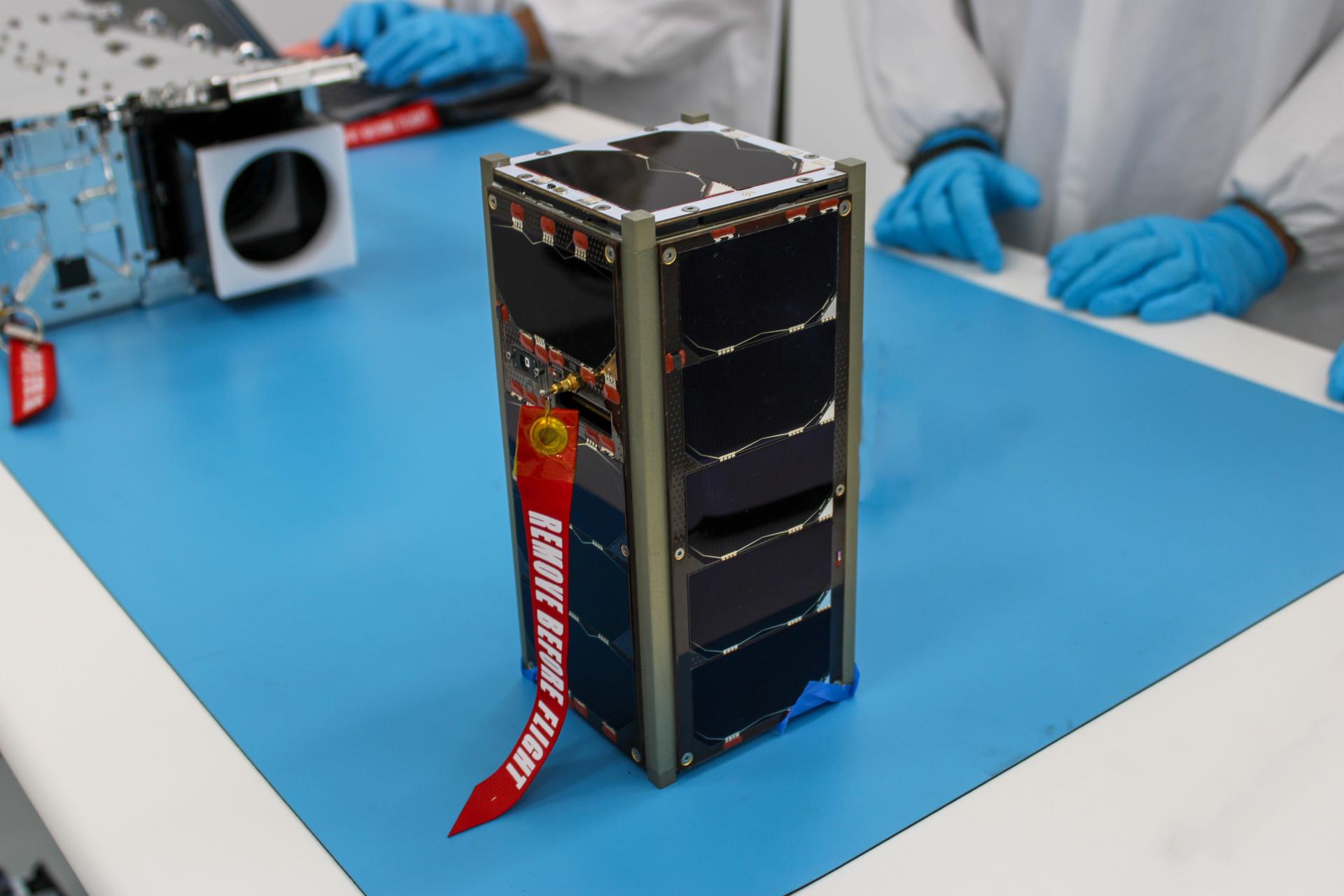
NASA’s ELaNa 43 Prepares for Firefly Aerospace Launch
Why scientists are intrigued by air in nasa’s mars sample tubes.
- Search All NASA Missions
- A to Z List of Missions
- Upcoming Launches and Landings
- Spaceships and Rockets
- Communicating with Missions
- James Webb Space Telescope
- Hubble Space Telescope
- Why Go to Space
- Commercial Space
- Destinations
- Living in Space
- Explore Earth Science
- Earth, Our Planet
- Earth Science in Action
- Earth Multimedia
- Earth Science Researchers
- Pluto & Dwarf Planets
- Asteroids, Comets & Meteors
- The Kuiper Belt
- The Oort Cloud
- Skywatching
- The Search for Life in the Universe
- Black Holes
- The Big Bang
- Dark Energy & Dark Matter
- Earth Science
- Planetary Science
- Astrophysics & Space Science
- The Sun & Heliophysics
- Biological & Physical Sciences
- Lunar Science
- Citizen Science
- Astromaterials
- Aeronautics Research
- Human Space Travel Research
- Science in the Air
- NASA Aircraft
- Flight Innovation
- Supersonic Flight
- Air Traffic Solutions
- Green Aviation Tech
- Drones & You
- Technology Transfer & Spinoffs
- Space Travel Technology
- Technology Living in Space
- Manufacturing and Materials
- Science Instruments
- For Kids and Students
- For Educators
- For Colleges and Universities
- For Professionals
- Science for Everyone
- Requests for Exhibits, Artifacts, or Speakers
- STEM Engagement at NASA
- NASA's Impacts
- Centers and Facilities
- Directorates
- Organizations
- People of NASA
- Internships
- Our History
- Doing Business with NASA
- Get Involved
- Aeronáutica
- Ciencias Terrestres
- Sistema Solar
- All NASA News
- Video Series on NASA+
- Newsletters
- Social Media
- Media Resources
- Upcoming Launches & Landings
- Virtual Events
- Sounds and Ringtones
- Interactives
- STEM Multimedia

Amendment 22: Heliophysics Flight Opportunities in Research and Technology Final Text and Due Date

Mercury Resources

Former Astronaut Charles M. Duke, Jr.

Lakita Lowe: Leading Space Commercialization Innovations and Fostering STEM Engagement

Former Astronaut Russell L. “Rusty” Schweickart

The Ocean and Climate Change
NASA Satellites Find Snow Didn’t Offset Southwest US Groundwater Loss

NASA-Led Mission to Map Air Pollution Over Both U.S. Coasts

Perseverance Finds Popcorn on Planet Mars

Hubble Captures Infant Stars Transforming a Nebula

First of Its Kind Detection Made in Striking New Webb Image

NASA Releases Hubble Image Taken in New Pointing Mode

Hypersonic Technology Project

NASA Engineer Honored as Girl Scouts ‘Woman of Distinction’

NASA, MagniX Altitude Tests Lay Groundwork for Hybrid Electric Planes

Augmented Reality Speeds Spacecraft Construction at NASA Goddard

Giant Batteries Deliver Renewable Energy When It’s Needed

Slow Your Student’s ‘Summer Slide’ and Beat Boredom With NASA STEM

Next Generation NASA Technologies Tested in Flight

Astronauta de la NASA Frank Rubio

Diez maneras en que los estudiantes pueden prepararse para ser astronautas

Astronauta de la NASA Marcos Berríos
What is earth’s energy budget five questions with a guy who knows.
Earth’s energy budget. Not a familiar concept? Maybe you’re scratching your head, wondering, what is that? Don’t worry. You’re not the only one.
The good news is: We have answers. And those answers come courtesy of Norman Loeb, an atmospheric scientist at NASA’s Langley Research Center in Hampton, Virginia. Loeb is the principal investigator for an experiment called the Clouds and the Earth’s Radiant Energy System (CERES). CERES instruments measure how much of the sun’s energy is reflected back to space and how much thermal energy is emitted by Earth to space. Five CERES instruments are on orbit aboard three satellites, and the CERES team at Langley is preparing to launch a sixth CERES instrument, CERES FM6, to orbit later this year.
We recently sent Loeb a few questions about the energy budget. These were his responses.
In the simplest terms possible, what is Earth’s energy budget?
Earth’s energy budget describes the balance between the radiant energy that reaches Earth from the sun and the energy that flows from Earth back out to space. Energy from the sun is mostly in the visible portion of the electromagnetic spectrum. About 30 percent of the sun’s incoming energy is reflected back to space by clouds, atmospheric molecules, tiny suspended particles called aerosols, and the Earth’s land, snow and ice surfaces. The Earth system also emits thermal radiant energy to space mainly in the infrared part of the electromagnetic spectrum. The intensity of thermal emission from a surface depends upon its temperature.
Why is it important for us to study the energy budget?
The Earth-atmosphere system is constantly trying to maintain a balance between the energy that reaches Earth from the sun and the energy that flows from Earth back out to space. If the Earth system is changed either through natural phenomena — such as volcanoes — or man’s activities and an imbalance in the Earth’s energy budget occurs, the Earth’s temperature will eventually increase or decrease in order to restore an energy balance.
Understanding exactly how the system is adjusting at any given time is complicated by internal variations in the system associated with atmospheric and oceanic circulations that also cause Earth’s energy budget to vary. To improve our understanding, observations of the Earth’s energy budget are necessary over a range of time scales, from monthly to multi-decadal.
The regional distribution across the globe of the difference between incoming and outgoing radiant energy drives the atmospheric and oceanic circulations. In the tropics, there is more energy absorbed than emitted, resulting in a surplus of radiant energy. At high latitudes, the opposite is true. In order to restore this latitudinal imbalance in radiant energy, the general circulation of the atmosphere and oceans transport heat from the tropics to the poles. A change in the regional distribution of radiant energy would therefore have a direct impact on weather and ocean circulation patterns.
The radiation balance at the Earth’s surface is also a critically important as it provides the energy needed to evaporate water at the surface, which in turn determines how much precipitation can fall over the globe.
How does CERES fit in?
The CERES project merges observations from multiple data sources to produce data products for the science community. CERES data products are used to understand how clouds and aerosols influence Earth’s energy budget from the top of the atmosphere down to the surface; to understand the trends and patterns of change associated with sea ice and snow cover in polar regions; to improve seasonal-to-interannual forecasts; and to provide surface radiation data for solar power, solar cooking, and architectural applications, as well as for the agricultural community.
Key to producing these data products is the CERES instrument, which measures how much of the sun’s energy is reflected back to space and how much thermal energy is emitted by Earth to space. CERES instruments provide global coverage daily at a high resolution. Currently, there are five CERES instruments in orbit taking measurements of Earth’s radiation budget. A sixth CERES instrument is scheduled to fly aboard the National Oceanic and Atmospheric Administration’s Joint Polar Satellite System (JPSS) satellite later this year.
The CERES project also uses imager measurements from the Moderate Resolution Imaging Spectroradiometer (MODIS) and the Visible Infrared Imaging Radiometer Suite (VIIRS) to provide additional information about the clouds, aerosols and surface properties observed by CERES. In addition, the CERES team uses geostationary imager measurements to provide information about how the radiation budget is varying between CERES observation times.
As far as naturally occurring phenomena and human activities are concerned, what are some of the primary impacts on the energy budget?
Although CERES instruments have been collecting data since 2000, this is still a relatively short record when considering change associated with human activities. Nevertheless, the CERES record has captured rather marked changes to the energy budget over the Arctic due to the rapid loss of sea ice associated with the warming of the Arctic. Within the tropics, the CERES data have captured marked variations in the Earth’s energy budget associated with the El Niño-Southern Oscillation (ENSO), which cause large variations in the energy budget at global scales.
What do you most enjoy about your job?
I enjoy working with a talented and smart group of scientists and engineers motivated by the need to provide the most accurate information about the Earth’s energy budget.
Navigation menu
Earth's energy budget, in other languages.
Earth's energy budget refers to the tracking of how much energy is flowing into and out of the Earth's climate , where the energy is going, and if the energy coming in balances with the energy going out. [1] Understanding the Earth's energy budget can help to predict future effects of global warming , and to understand the various flows of energy on the Earth . Additionally, knowing how Earth's energy budget balances can provide insight into how the energy from the Sun interacts with the atmosphere . For example, this is important when examining the affects of greenhouse gases in the atmosphere—to ensure conditions on Earth are habitable. For the energy budget to balance, all that needs to occur is:
Earth's Energy Balance
The two major components that must be investigated to determine if the Earth's energy budget balances is the incoming energy from the Sun and the outgoing infrared radiation from the Earth and its atmosphere. Looking at the energy flows that occur between the atmosphere and the surface of the Earth can help to understand how the Earth's energy budget is balanced. Figure 1 shows the current understanding of how energy flows generally look on the Earth.
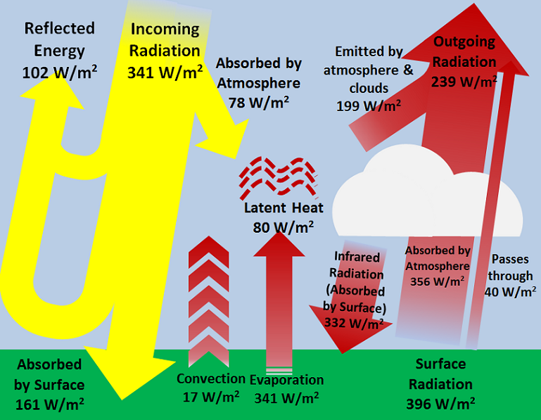
Earth's energy budget is vital in establishing the Earth's climate. When the energy budget balances, the temperature on the Earth stays relatively constant, with no overall increase or decrease in average temperature. The energy coming in to the Earth comes from the Sun, and over the surface of the planet this incoming radiation has a rate of transport of [math]341 \frac{W}{m^2}[/math] . A thorough explanation of how this value is determined can be found here .
However, not all of this energy reaches the Earth's atmosphere or surface as some is reflected by clouds or the atmosphere. The energy that does pass through is absorbed by the atmosphere or the surface, and then moves around through convection , evaporation , or in the form of latent heat . [3] Finally, when the energy exits the Earth it can do so by emission from the surface of the Earth, by clouds, or by the atmosphere. Some of the energy that is radiated by the surface of the Earth is absorbed by clouds and greenhouse gases in the atmosphere and then re-emitted downwards, which is how the surface of the Earth is heated and kept at a habitable temperature. This process of heating is known as the greenhouse effect . Overall, the energy that exits the Earth in different forms, when added together is equal to the energy that is absorbed by different parts of the Earth.
Earth's Energy Imbalance
The incoming energy to the Earth and the outgoing energy from the Earth do not actually balance. This imbalance is partially caused by the incoming energy from the Sun—which varies with the seasons and changes in the composition of the Earth's atmosphere. [4] Changes in the composition of Earth's atmosphere alters the quantity of energy absorbed and reflected by the atmosphere seen in Figure 1. Changing factors such as these result in a very small, but significant energy imbalance on the Earth.
As human activities increase the amount of carbon dioxide in the atmosphere, the energy imbalance continues to grow. Today, the energy imbalance amounts to approximately [math]0.9 \frac{W}{m^2}[/math] . This means that more energy is coming in (and being absorbed) than is leaving the Earth. [4] Compared to flow values in the hundreds of watts per meter squared, this imbalance seems negligible. However, to account for this imbalance, the Earth's temperature will increase in response. As well, since the amounts of carbon dioxide and other greenhouse gases in our atmosphere are increasing, this value is projected to increase at a rate of [math]0.3 \frac{W}{m^2}[/math] per decade, contributing even more to increasing temperatures. [5] It is this imbalance in the energy budget that results in increasing temperatures on the Earth, one of the most significant effects of climate change .
- ↑ John Cook, Hayden Washington. (May 8, 2015). Climate Change Denial: Heads in the Sand , 1st Edition. Washington, DC, Earthscan 2011.
- ↑ Created internally by a member of the Energy Education team. Adapted from: R. Wolfson, Figure 12.5 in Energy, Environment and Climate , 2nd ed. New York, U.S.A.: Norton, 2012, pp. 331
- ↑ NASA Earth Observatory. (May 8, 2015). Climate and Earth's Energy Budget [Online]. Available: http://earthobservatory.nasa.gov/Features/EnergyBalance
- ↑ 4.0 4.1 R. Wolfson, (May 8, 2015). Energy, Environment and Climate , 2nd ed. New York, U.S.A.: Norton, 2012.
- ↑ M. Balmaseda, J.Fasullo, and E. Trenberth. (May 8, 2015). Earth's Energy Imbalance [Online]. Available: http://www.cgd.ucar.edu/staff/trenbert/trenberth.papers/T_F_B_energyImb_JCLI_14.pdf
- EO Explorer
- Global Maps
Climate and Earth’s Energy Budget
The Earth’s climate is a solar powered system. Globally, over the course of the year, the Earth system—land surfaces, oceans, and atmosphere—absorbs an average of about 240 watts of solar power per square meter (one watt is one joule of energy every second). The absorbed sunlight drives photosynthesis, fuels evaporation, melts snow and ice, and warms the Earth system.

Solar power drives Earth’s climate. Energy from the Sun heats the surface, warms the atmosphere, and powers the ocean currents. (Astronaut photograph ISS015-E-10469, courtesy NASA/JSC Gateway to Astronaut Photography of Earth. )
The Sun doesn’t heat the Earth evenly. Because the Earth is a sphere, the Sun heats equatorial regions more than polar regions. The atmosphere and ocean work non-stop to even out solar heating imbalances through evaporation of surface water, convection, rainfall, winds, and ocean circulation. This coupled atmosphere and ocean circulation is known as Earth’s heat engine.
The climate’s heat engine must not only redistribute solar heat from the equator toward the poles, but also from the Earth’s surface and lower atmosphere back to space. Otherwise, Earth would endlessly heat up. Earth’s temperature doesn’t infinitely rise because the surface and the atmosphere are simultaneously radiating heat to space. This net flow of energy into and out of the Earth system is Earth’s energy budget.

When the flow of incoming solar energy is balanced by an equal flow of heat to space, Earth is in radiative equilibrium, and global temperature is relatively stable. Anything that increases or decreases the amount of incoming or outgoing energy disturbs Earth’s radiative equilibrium; global temperatures rise or fall in response.
Incoming Sunlight
All matter in the universe that has a temperature above absolute zero (the temperature at which all atomic or molecular motion stops) radiates energy across a range of wavelengths in the electromagnetic spectrum. The hotter something is, the shorter its peak wavelength of radiated energy is. The hottest objects in the universe radiate mostly gamma rays and x-rays. Cooler objects emit mostly longer-wavelength radiation, including visible light, thermal infrared, radio, and microwaves.

The Sun’s surface temperature is 5,500° C, and its peak radiation is in visible wavelengths of light. Earth’s effective temperature—the temperature it appears when viewed from space—is -20° C, and it radiates energy that peaks in thermal infrared wavelengths. (Illustration adapted from Robert Rohde. )

Incandescent light bulbs radiate 40 to 100 watts. The Sun delivers 1,360 watts per square meter. An astronaut facing the Sun has a surface area of about 0.85 square meters, so he or she receives energy equivalent to 19 60-watt light bulbs. (Photograph ©2005 Paul Watson. )
The surface of the Sun has a temperature of about 5,800 Kelvin (about 5,500 degrees Celsius, or about 10,000 degrees Fahrenheit). At that temperature, most of the energy the Sun radiates is visible and near-infrared light. At Earth’s average distance from the Sun (about 150 million kilometers), the average intensity of solar energy reaching the top of the atmosphere directly facing the Sun is about 1,360 watts per square meter, according to measurements made by the most recent NASA satellite missions. This amount of power is known as the total solar irradiance. (Before scientists discovered that it varies by a small amount during the sunspot cycle, total solar irradiance was sometimes called “the solar constant.”)
A watt is measurement of power, or the amount of energy that something generates or uses over time. How much power is 1,360 watts? An incandescent light bulb uses anywhere from 40 to 100 watts. A microwave uses about 1000 watts. If for just one hour, you could capture and re-use all the solar energy arriving over a single square meter at the top of the atmosphere directly facing the Sun—an area no wider than an adult’s outstretched arm span—you would have enough to run a refrigerator all day.
The total solar irradiance is the maximum possible power that the Sun can deliver to a planet at Earth’s average distance from the Sun; basic geometry limits the actual solar energy intercepted by Earth. Only half the Earth is ever lit by the Sun at one time, which halves the total solar irradiance.

Energy from sunlight is not spread evenly over Earth. One hemisphere is always dark, receiving no solar radiation at all. On the daylight side, only the point directly under the Sun receives full-intensity solar radiation. From the equator to the poles, the Sun’ rays meet Earth at smaller and smaller angles, and the light gets spread over larger and larger surface areas (red lines). (NASA illustration by Robert Simmon.)
In addition, the total solar irradiance is the maximum power the Sun can deliver to a surface that is perpendicular to the path of incoming light. Because the Earth is a sphere, only areas near the equator at midday come close to being perpendicular to the path of incoming light. Everywhere else, the light comes in at an angle. The progressive decrease in the angle of solar illumination with increasing latitude reduces the average solar irradiance by an additional one-half.

The solar radiation received at Earth’s surface varies by time and latitude. This graph illustrates the relationship between latitude, time, and solar energy during the equinoxes. The illustrations show how the time of day (A-E) affects the angle of incoming sunlight (revealed by the length of the shadow) and the light’s intensity. On the equinoxes, the Sun rises at 6:00 a.m. everywhere. The strength of sunlight increases from sunrise until noon, when the Sun is directly overhead along the equator (casting no shadow). After noon, the strength of sunlight decreases until the Sun sets at 6:00 p.m. The tropics (from 0 to 23.5° latitude) receive about 90% of the energy compared to the equator, the mid-latitudes (45°) roughly 70%, and the Arctic and Antarctic Circles about 40%. (NASA illustration by Robert Simmon.)
Averaged over the entire planet, the amount of sunlight arriving at the top of Earth’s atmosphere is only one-fourth of the total solar irradiance, or approximately 340 watts per square meter.
When the flow of incoming solar energy is balanced by an equal flow of heat to space, Earth is in radiative equilibrium, and global temperature is relatively stable. Anything that increases or decreases the amount of incoming or outgoing energy disturbs Earth’s radiative equilibrium; global temperatures must rise or fall in response.
Heating Imbalances
Three hundred forty watts per square meter of incoming solar power is a global average; solar illumination varies in space and time. The annual amount of incoming solar energy varies considerably from tropical latitudes to polar latitudes (described on page 2). At middle and high latitudes, it also varies considerably from season to season.

The peak energy received at different latitudes changes throughout the year. This graph shows how the solar energy received at local noon each day of the year changes with latitude. At the equator (gray line), the peak energy changes very little throughout the year. At high northern (blue lines) and southern (green) latitudes, the seasonal change is extreme. (NASA illustration by Robert Simmon.)
If the Earth’s axis of rotation were vertical with respect to the path of its orbit around the Sun, the size of the heating imbalance between equator and the poles would be the same year round, and the seasons we experience would not occur. Instead Earth’s axis is tilted off vertical by about 23 degrees. As the Earth orbits the Sun, the tilt causes one hemisphere and then the other to receive more direct sunlight and to have longer days.

The total energy received each day at the top of the atmosphere depends on latitude. The highest daily amounts of incoming energy (pale pink) occur at high latitudes in summer, when days are long, rather than at the equator. In winter, some polar latitudes receive no light at all (black). The Southern Hemisphere receives more energy during December (southern summer) than the Northern Hemisphere does in June (northern summer) because Earth’s orbit is not a perfect circle and Earth is slightly closer to the Sun during that part of its orbit. Total energy received ranges from 0 (during polar winter) to about 50 (during polar summer) megajoules per square meter per day.
In the “summer hemisphere,” the combination of more direct sunlight and longer days means the pole can receive more incoming sunlight than the tropics, but in the winter hemisphere, it gets none. Even though illumination increases at the poles in the summer, bright white snow and sea ice reflect a significant portion of the incoming light, reducing the potential solar heating.

The amount of sunlight the Earth absorbs depends on the reflectivness of the atmosphere and the ground surface. This satellite map shows the amount of solar radiation (watts per square meter) reflected during September 2008. Along the equator, clouds reflected a large proportion of sunlight, while the pale sands of the Sahara caused the high reflectivness in North Africa. Neither pole is receiving much incoming sunlight at this time of year, so they reflect little energy even though both are ice-covered. (NASA map by Robert Simmon, based on CERES data.)
The differences in reflectivness (albedo) and solar illumination at different latitudes lead to net heating imbalances throughout the Earth system. At any place on Earth, the net heating is the difference between the amount of incoming sunlight and the amount heat radiated by the Earth back to space (for more on this energy exchange see Page 4 ). In the tropics there is a net energy surplus because the amount of sunlight absorbed is larger than the amount of heat radiated. In the polar regions, however, there is an annual energy deficit because the amount of heat radiated to space is larger than the amount of absorbed sunlight.

This map of net radiation (incoming sunlight minus reflected light and outgoing heat) shows global energy imbalances in September 2008, the month of an equinox. Areas around the equator absorbed about 200 watts per square meter more on average (orange and red) than they reflected or radiated. Areas near the poles reflected and/or radiated about 200 more watts per square meter (green and blue) than they absorbed. Mid-latitudes were roughly in balance. (NASA map by Robert Simmon, based on CERES data.)
The net heating imbalance between the equator and poles drives an atmospheric and oceanic circulation that climate scientists describe as a “heat engine.” (In our everyday experience, we associate the word engine with automobiles, but to a scientist, an engine is any device or system that converts energy into motion.) The climate is an engine that uses heat energy to keep the atmosphere and ocean moving. Evaporation, convection, rainfall, winds, and ocean currents are all part of the Earth’s heat engine.
Earth’s Energy Budget
Note: Determining exact values for energy flows in the Earth system is an area of ongoing climate research. Different estimates exist, and all estimates have some uncertainty. Estimates come from satellite observations, ground-based observations, and numerical weather models. The numbers in this article rely most heavily on direct satellite observations of reflected sunlight and thermal infrared energy radiated by the atmosphere and the surface.
Earth’s heat engine does more than simply move heat from one part of the surface to another; it also moves heat from the Earth’s surface and lower atmosphere back to space. This flow of incoming and outgoing energy is Earth’s energy budget. For Earth’s temperature to be stable over long periods of time, incoming energy and outgoing energy have to be equal. In other words, the energy budget at the top of the atmosphere must balance. This state of balance is called radiative equilibrium.
About 29 percent of the solar energy that arrives at the top of the atmosphere is reflected back to space by clouds, atmospheric particles, or bright ground surfaces like sea ice and snow. This energy plays no role in Earth’s climate system. About 23 percent of incoming solar energy is absorbed in the atmosphere by water vapor, dust, and ozone, and 48 percent passes through the atmosphere and is absorbed by the surface. Thus, about 71 percent of the total incoming solar energy is absorbed by the Earth system.

Of the 340 watts per square meter of solar energy that falls on the Earth, 29% is reflected back into space, primarily by clouds, but also by other bright surfaces and the atmosphere itself. About 23% of incoming energy is absorbed in the atmosphere by atmospheric gases, dust, and other particles. The remaining 48% is absorbed at the surface. (NASA illustration by Robert Simmon. Astronaut photograph ISS013-E-8948. )
When matter absorbs energy, the atoms and molecules that make up the material become excited; they move around more quickly. The increased movement raises the material’s temperature. If matter could only absorb energy, then the temperature of the Earth would be like the water level in a sink with no drain where the faucet runs continuously.
Temperature doesn’t infinitely rise, however, because atoms and molecules on Earth are not just absorbing sunlight, they are also radiating thermal infrared energy (heat). The amount of heat a surface radiates is proportional to the fourth power of its temperature. If temperature doubles, radiated energy increases by a factor of 16 (2 to the 4th power). If the temperature of the Earth rises, the planet rapidly emits an increasing amount of heat to space. This large increase in heat loss in response to a relatively smaller increase in temperature—referred to as radiative cooling—is the primary mechanism that prevents runaway heating on Earth.

Absorbed sunlight is balanced by heat radiated from Earth’s surface and atmosphere. This satellite map shows the distribution of thermal infrared radiation emitted by Earth in September 2008. Most heat escaped from areas just north and south of the equator, where the surface was warm, but there were few clouds. Along the equator, persistent clouds prevented heat from escaping. Likewise, the cold poles radiated little heat. (NASA map by Robert Simmon, based on CERES data.)
The atmosphere and the surface of the Earth together absorb 71 percent of incoming solar radiation, so together, they must radiate that much energy back to space for the planet’s average temperature to remain stable. However, the relative contribution of the atmosphere and the surface to each process (absorbing sunlight versus radiating heat) is asymmetric. The atmosphere absorbs 23 percent of incoming sunlight while the surface absorbs 48. The atmosphere radiates heat equivalent to 59 percent of incoming sunlight; the surface radiates only 12 percent. In other words, most solar heating happens at the surface, while most radiative cooling happens in the atmosphere. How does this reshuffling of energy between the surface and atmosphere happen?
Surface Energy Budget
To understand how the Earth’s climate system balances the energy budget, we have to consider processes occurring at the three levels: the surface of the Earth, where most solar heating takes place; the edge of Earth’s atmosphere, where sunlight enters the system; and the atmosphere in between. At each level, the amount of incoming and outgoing energy, or net flux, must be equal.
Remember that about 29 percent of incoming sunlight is reflected back to space by bright particles in the atmosphere or bright ground surfaces, which leaves about 71 percent to be absorbed by the atmosphere (23 percent) and the land (48 percent). For the energy budget at Earth’s surface to balance, processes on the ground must get rid of the 48 percent of incoming solar energy that the ocean and land surfaces absorb. Energy leaves the surface through three processes: evaporation, convection, and emission of thermal infrared energy.

The surface absorbs about 48% of incoming sunlight. Three processes remove an equivalent amount of energy from the Earth’s surface: evaporation (25%), convection (5%), and thermal infrared radiation, or heat (net 17%). (NASA illustration by Robert Simmon. Photograph ©2006 Cyron. )
About 25 percent of incoming solar energy leaves the surface through evaporation. Liquid water molecules absorb incoming solar energy, and they change phase from liquid to gas. The heat energy that it took to evaporate the water is latent in the random motions of the water vapor molecules as they spread through the atmosphere. When the water vapor molecules condense back into rain, the latent heat is released to the surrounding atmosphere. Evaporation from tropical oceans and the subsequent release of latent heat are the primary drivers of the atmospheric heat engine (described on page 3 ).

Towers of cumulus clouds transport energy away from the surface of the Earth. Solar heating drives evaporation. Warm, moist air becomes buoyant and rises, moving energy from the surface high into the atmosphere. Energy is released back into the atmosphere when the water vapor condenses into liquid water or freezes into ice crystals. (Astronaut Photograph ISS006-E-19436. )
An additional 5 percent of incoming solar energy leaves the surface through convection. Air in direct contact with the sun-warmed ground becomes warm and buoyant. In general, the atmosphere is warmer near the surface and colder at higher altitudes, and under these conditions, warm air rises, shuttling heat away from the surface.
Finally, a net of about 17 percent of incoming solar energy leaves the surface as thermal infrared energy (heat) radiated by atoms and molecules on the surface. This net upward flux results from two large but opposing fluxes: heat flowing upward from the surface to the atmosphere (117%) and heat flowing downward from the atmosphere to the ground (100%). (These competing fluxes are part of the greenhouse effect, described on page 6. ) Remember that the peak wavelength of energy a surface radiates is based on its temperature. The Sun’s peak radiation is at visible and near-infrared wavelengths. The Earth’s surface is much cooler, only about 15 degrees Celsius on average. The peak radiation from the surface is at thermal infrared wavelengths around 12.5 micrometers.
The Atmosphere’s Energy Budget
Just as the incoming and outgoing energy at the Earth’s surface must balance, the flow of energy into the atmosphere must be balanced by an equal flow of energy out of the atmosphere and back to space. Satellite measurements indicate that the atmosphere radiates thermal infrared energy equivalent to 59 percent of the incoming solar energy. If the atmosphere is radiating this much, it must be absorbing that much. Where does that energy come from?
Clouds, aerosols, water vapor, and ozone directly absorb 23 percent of incoming solar energy. Evaporation and convection transfer 25 and 5 percent of incoming solar energy from the surface to the atmosphere. These three processes transfer the equivalent of 53 percent of the incoming solar energy to the atmosphere. If total inflow of energy must match the outgoing thermal infrared observed at the top of the atmosphere, where does the remaining fraction (about 5-6 percent) come from? The remaining energy comes from the Earth’s surface.
The Natural Greenhouse Effect
Just as the major atmospheric gases (oxygen and nitrogen) are transparent to incoming sunlight, they are also transparent to outgoing thermal infrared. However, water vapor, carbon dioxide, methane, and other trace gases are opaque to many wavelengths of thermal infrared energy. Remember that the surface radiates the net equivalent of 17 percent of incoming solar energy as thermal infrared. However, the amount that directly escapes to space is only about 12 percent of incoming solar energy. The remaining fraction—a net 5-6 percent of incoming solar energy—is transferred to the atmosphere when greenhouse gas molecules absorb thermal infrared energy radiated by the surface.

The atmosphere radiates the equivalent of 59% of incoming sunlight back to space as thermal infrared energy, or heat. Where does the atmosphere get its energy? The atmosphere directly absorbs about 23% of incoming sunlight, and the remaining energy is transferred from the Earth’s surface by evaporation (25%), convection (5%), and thermal infrared radiation (a net of 5-6%). The remaining thermal infrared energy from the surface (12%) passes through the atmosphere and escapes to space. (NASA illustration by Robert Simmon. Astronaut photograph ISS017-E-13859. )
When greenhouse gas molecules absorb thermal infrared energy, their temperature rises. Like coals from a fire that are warm but not glowing, greenhouse gases then radiate an increased amount of thermal infrared energy in all directions. Heat radiated upward continues to encounter greenhouse gas molecules; those molecules absorb the heat, their temperature rises, and the amount of heat they radiate increases. At an altitude of roughly 5-6 kilometers, the concentration of greenhouse gases in the overlying atmosphere is so small that heat can radiate freely to space.
Because greenhouse gas molecules radiate heat in all directions, some of it spreads downward and ultimately comes back into contact with the Earth’s surface, where it is absorbed. The temperature of the surface becomes warmer than it would be if it were heated only by direct solar heating. This supplemental heating of the Earth’s surface by the atmosphere is the natural greenhouse effect.
Effect on Surface Temperature
The natural greenhouse effect raises the Earth’s surface temperature to about 15 degrees Celsius on average—more than 30 degrees warmer than it would be if it didn’t have an atmosphere. The amount of heat radiated from the atmosphere to the surface (sometimes called “back radiation”) is equivalent to 100 percent of the incoming solar energy. The Earth’s surface responds to the “extra” (on top of direct solar heating) energy by raising its temperature.

On average, 340 watts per square meter of solar energy arrives at the top of the atmosphere. Earth returns an equal amount of energy back to space by reflecting some incoming light and by radiating heat (thermal infrared energy). Most solar energy is absorbed at the surface, while most heat is radiated back to space by the atmosphere. Earth's average surface temperature is maintained by two large, opposing energy fluxes between the atmosphere and the ground (right)—the greenhouse effect. NASA illustration by Robert Simmon, adapted from Trenberth et al. 2009, using CERES flux estimates provided by Norman Loeb.)
Why doesn’t the natural greenhouse effect cause a runaway increase in surface temperature? Remember that the amount of energy a surface radiates always increases faster than its temperature rises—outgoing energy increases with the fourth power of temperature. As solar heating and “back radiation” from the atmosphere raise the surface temperature, the surface simultaneously releases an increasing amount of heat—equivalent to about 117 percent of incoming solar energy. The net upward heat flow, then, is equivalent to 17 percent of incoming sunlight (117 percent up minus 100 percent down).
Some of the heat escapes directly to space, and the rest is transferred to higher and higher levels of the atmosphere, until the energy leaving the top of the atmosphere matches the amount of incoming solar energy. Because the maximum possible amount of incoming sunlight is fixed by the solar constant (which depends only on Earth’s distance from the Sun and very small variations during the solar cycle), the natural greenhouse effect does not cause a runaway increase in surface temperature on Earth.
Climate Forcings and Global Warming
Any changes to the Earth’s climate system that affect how much energy enters or leaves the system alters Earth’s radiative equilibrium and can force temperatures to rise or fall. These destabilizing influences are called climate forcings. Natural climate forcings include changes in the Sun’s brightness, Milankovitch cycles (small variations in the shape of Earth’s orbit and its axis of rotation that occur over thousands of years), and large volcanic eruptions that inject light-reflecting particles as high as the stratosphere. Manmade forcings include particle pollution (aerosols), which absorb and reflect incoming sunlight; deforestation, which changes how the surface reflects and absorbs sunlight; and the rising concentration of atmospheric carbon dioxide and other greenhouse gases, which decrease heat radiated to space. A forcing can trigger feedbacks that intensify or weaken the original forcing. The loss of ice at the poles, which makes them less reflective, is an example of a feedback.

Carbon dioxide forces the Earth’s energy budget out of balance by absorbing thermal infrared energy (heat) radiated by the surface. It absorbs thermal infrared energy with wavelengths in a part of the energy spectrum that other gases, such as water vapor, do not. Although water vapor is a powerful absorber of many wavelengths of thermal infrared energy, it is almost transparent to others. The transparency at those wavelengths is like a window the atmosphere leaves open for radiative cooling of the Earth’s surface. The most important of these “water vapor windows” is for thermal infrared with wavelengths centered around 10 micrometers. (The maximum transparency occurs at 10 micrometers, but partial transparency occurs for wavelengths between about 8 and about 14 micrometers.)
Carbon dioxide is a very strong absorber of thermal infrared energy with wavelengths longer than 12-13 micrometers, which means that increasing concentrations of carbon dioxide partially “close” the atmospheric window. In other words, wavelengths of outgoing thermal infrared energy that our atmosphere’s most abundant greenhouse gas—water vapor—would have let escape to space are instead absorbed by carbon dioxide.

All atmospheric gases have a unique pattern of energy absorption: they absorb some wavelengths of energy but are transparent to others. The absorption patterns of water vapor (blue peaks) and carbon dioxide (pink peaks) overlap in some wavelengths. Carbon dioxide is not as strong a greenhouse gas as water vapor, but it absorbs energy in wavelengths (12-15 micrometers) that water vapor does not, partially closing the “window” through which heat radiated by the surface would normally escape to space. (Illustration adapted from Robert Rohde. )
The absorption of outgoing thermal infrared by carbon dioxide means that Earth still absorbs about 70 percent of the incoming solar energy, but an equivalent amount of heat is no longer leaving. The exact amount of the energy imbalance is very hard to measure, but it appears to be a little over 0.8 watts per square meter. The imbalance is inferred from a combination of measurements, including satellite and ocean-based observations of sea level rise and warming.
When a forcing like increasing greenhouse gas concentrations bumps the energy budget out of balance, it doesn’t change the global average surface temperature instantaneously. It may take years or even decades for the full impact of a forcing to be felt. This lag between when an imbalance occurs and when the impact on surface temperature becomes fully apparent is mostly because of the immense heat capacity of the global ocean. The heat capacity of the oceans gives the climate a thermal inertia that can make surface warming or cooling more gradual, but it can’t stop a change from occurring.
The changes we have seen in the climate so far are only part of the full response we can expect from the current energy imbalance, caused only by the greenhouse gases we have released so far. Global average surface temperature has risen between 0.6 and 0.9 degrees Celsius in the past century, and it will likely rise at least 0.6 degrees in response to the existing energy imbalance.
As the surface temperature rises, the amount of heat the surface radiates will increase rapidly (see description of radiative cooling on Page 4). If the concentration of greenhouse gases stabilizes, then Earth’s climate will once again come into equilibrium, albeit with the “thermostat”—global average surface temperature—set at a higher temperature than it was before the Industrial Revolution.
However, as long as greenhouse gas concentrations continue to rise, the amount of absorbed solar energy will continue to exceed the amount of thermal infrared energy that can escape to space. The energy imbalance will continue to grow, and surface temperatures will continue to rise.
- Cahalan, R. (n.d.) Solar and Earth Radiation. Accessed December 12, 2008.
- Hansen, J., Nazarenko, L., Ruedy, R., Sato, M., Willis, J., Del Genio, A., Koch, D., Lacis, A., Lo, K., Menon, S., Novakov, T., Perlwitz, J., Russell, G., Schmidt, G.A., and Tausnev, N. (2005). Earth’s Energy Imbalance: Confirmation and Implications. Science, (308) 1431-1435.
- Kushnir, Y. (2000). Solar Radiation and the Earth’s Energy Balance. Published on The Climate System, complete online course material from the Department of Earth and Environmental Sciences at Columbia University. Accessed December 12, 2008.
- Peixoto, J., and Oort, A. (1992). Chapter 6: Radiation balance. In Physics of Climate (pp. 91-130). Woodbury, NY: American Institute of Physics Press.
- Peixoto, J., and Oort, A. (1992). Chapter 14: The ocean-atmosphere heat engine. In Physics of Climate (pp. 365-400). Woodbury, NY: American Institute of Physics Press.
- Marshall, J., and Plumb, R.A. (2008). Chapter 2: The global energy balance. In Atmosphere, Ocean, and Climate Dynamics: an Introductory Text (pp. 9-22).
- Marshall, J., and Plumb, R.A. (2008). Chapter 4: Convection. In Atmosphere, Ocean, and Climate Dynamics: an Introductory Text (pp. 31-60).
- Marshall, J., and Plumb, R.A. (2008). Chapter 8: The general circulation of the atmosphere. In Atmosphere, Ocean, and Climate Dynamics: an Introductory Text (pp. 139-161).
- Trenberth, K., Fasullo, J., Kiehl, J. (2009). Earth’s global energy budget. Bulletin of the American Meteorological Society.
Chapter 7: The Earth’s Energy Budget, Climate Feedbacks, and Climate Sensitivity
Coordinating Lead Authors:
Piers Forster (United Kingdom), Trude Storelvmo (Norway)
Lead Authors:
Kyle Armour (United States of America), William Collins (United Kingdom), Jean-Louis Dufresne (France), David Frame (New Zealand), Daniel J. Lunt (United Kingdom), Thorsten Mauritsen (Sweden/Denmark), Matthew D. Palmer (United Kingdom), Masahiro Watanabe (Japan), Martin Wild (Switzerland), Hua Zhang (China)
Contributing Authors:
Kari Alterskjær (Norway), Chris Smith (United Kingdom), Govindasamy Bala (India/United States of America), Nicolas Bellouin (United Kingdom/France), Terje Berntsen (Norway), Fábio Boeira Dias (Finland/Brazil), Sandrine Bony (France), Natalie J. Burls (United States of America/South Africa), Michelle Cain (United Kingdom), Catia M. Domingues (Australia, United Kingdom/Brazil), Aaron Donohoe (United States of America), Mark Flanner (United States of America), Jan S. Fuglestvedt (Norway), Lily C. Hahn (United States of America), Glen R. Harris (United Kingdom/New Zealand, United Kingdom), Christopher Jones (United Kingdom), Seiji Kato (United States of America), Jared Lewis (Australia/New Zealand), Zhanqing Li (United States of America), Mike Lockwood (United Kingdom), Norman Loeb (United States of America), Jochem Marotzke (Germany), Malte Meinshausen (Australia/Germany), Sebastian Milinski (Germany), Zebedee R.J. Nicholls (Australia), Ryan S. Padron Flasher (Switzerland/Ecuador, United States of America), Anna Possner (Germany), Cristian Proistosescu (Romania), Johannes Quaas (Germany), Joeri Rogelj (United Kingdom/Belgium), Daniel Rosenfeld (Israel), Bjørn H. Samset (Norway), Abhishek Savita (Australia/India), Jessica Vial (France), Karina von Schuckmann (France/Germany), Mark Zelinka (United States of America), Shuyun Zhao (China)
Review Editors:
Robert Colman (Australia), H. Damon Matthews (Canada), Venkatachalam Ramaswamy (United States of America)
Chapter Scientists:
Kari Alterskjær (Norway), Chris Smith (United Kingdom)
Figure 7.1a

Figure 7.1b

Figure 7.10

Figure 7.11

Figure 7.12

Figure 7.13

Figure 7.14

Figure 7.15

Figure 7.16

Figure 7.17

Figure 7.18

Figure 7.19

Figure 7.20

Figure 7.21

Figure 7.22

Box 7.1, Figure 1

Box 7.2, Figure 1

Cross-Chapter Box 7.1, Figure 1

FAQ 7.1 Figure 1

FAQ 7.2, Figure 1

FAQ 7.3, Figure 1

This chapter should be cited as:
Forster, P., T. Storelvmo, K. Armour, W. Collins, J.-L. Dufresne, D. Frame, D.J. Lunt, T. Mauritsen, M.D. Palmer, M. Watanabe, M. Wild, and H. Zhang, 2021: The Earth’s Energy Budget, Climate Feedbacks, and Climate Sensitivity. In Climate Change 2021: The Physical Science Basis. Contribution of Working Group I to the Sixth Assessment Report of the Intergovernmental Panel on Climate Change [Masson-Delmotte, V., P. Zhai, A. Pirani, S.L. Connors, C. Péan, S. Berger, N. Caud, Y. Chen, L. Goldfarb, M.I. Gomis, M. Huang, K. Leitzell, E. Lonnoy, J.B.R. Matthews, T.K. Maycock, T. Waterfield, O. Yelekçi, R. Yu, and B. Zhou (eds.)]. Cambridge University Press, Cambridge, United Kingdom and New York, NY, USA, pp. 923–1054, doi: 10.1017/9781009157896.009 .
Executive Summary Expand section
This chapter assesses the present state of knowledge of Earth’s energy budget: that is, the main flows of energy into and out of the Earth system, and how these energy flows govern the climate response to a radiative forcing. Changes in atmospheric composition and land use, like those caused by anthropogenic greenhouse gas emissions and emissions of aerosols and their precursors, affect climate through perturbations to Earth’s top-of-atmosphere energy budget. The effective radiative forcings (ERFs) quantify these perturbations, including any consequent adjustment to the climate system (but excluding surface temperature response). How the climate system responds to a given forcing is determined by climate feedbacks associated with physical, biogeophysical and biogeochemical processes. These feedback processes are assessed, as are useful measures of global climate response, namely equilibrium climate sensitivity (ECS) and the transient climate response (TCR). This chapter also assesses emissions metrics, which are used to quantify how the climate response to the emissions of different greenhouse gases compares to the response to the emissions of carbon dioxide (CO 2 ). This chapter builds on the assessment of carbon cycle and aerosol processes from Chapters 5 and 6, respectively, to quantify non-CO 2 biogeochemical feedbacks and the ERF for aerosols. Other chapters in this Report use this chapter’s assessment of ERF, ECS and TCR to help understand historical and future temperature changes (Chapters 3 and 4, respectively), the response to cumulative emissions and the remaining carbon budget (Chapter 5), emissions-based radiative forcing (Chapter 6) and sea level rise (Chapter 9). This chapter builds on findings from the IPCC Fifth Assessment Report (AR5), the Special Report on Global Warming of 1.5°C (SR1.5), the Special Report on the Ocean and Cryosphere in a Changing Climate (SROCC) and the Special Report on climate change, desertification, land degradation, sustainable land management, food security, and greenhouse gas luxes in terrestrial ecosystems (SRCCL). Very likely ranges are presented unless otherwise indicated.
Earth’s Energy Budget
Since AR5, the accumulation of energy in the Earth system, quantified by changes in the global energy inventory for all components of the climate system, has become established as a robust measure of the rate of global climate change on interannual-to-decadal time scales. Compared to changes in global surface air temperature (GSAT), the global energy inventory exhibits less variability, which can mask underlying climate trends. Compared to AR5, there is increased confidence in the quantification of changes in the global energy inventory due to improved observational records and closure of the sea level budget. Energy will continue to accumulate in the Earth system until at least the end of the 21st century, even under strong mitigation scenarios, and will primarily be observed through ocean warming and associated with continued sea level rise through thermal expansion ( high confidence ). {7.2.2, Box 7.2, Table 7.1, Cross-Chapter Box 9.1, Table 9.5, 9.2.2, 9.6.3}
The global energy inventory increased by 282 [177 to 387] Zettajoules (ZJ; 10 21 Joules) for the period 19 71–200 6 and 152 [100 to 205] ZJ for the period 2006–2018. This corresponds to an Earth energy imbalance of 0.50 [0.32 to 0.69] W m –2 for the period 1971–2006, increasing to 0.79 [0.52 to 1.06] W m –2 for the period 2006–2018, expressed per unit area of Earth’s surface. Ocean heat uptake is by far the largest contribution and accounts for 91% of the total energy change. Compared to AR5, the contribution from land heating has been revised upwards from about 3% to about 5%. Melting of ice and warming of the atmosphere account for about 3% and 1% of the total change respectively. More comprehensive analysis of inventory components and cross-validation of global heating rates from satellite and in situ observations lead to a strengthened assessment relative to AR5 ( high confidence ). {Box 7.2, 7.2.2, Table 7.1, 7.5.2.3}
Improved quantification of effective radiative forcing, the climate system radiative response, and the observed energy increase in the Earth system for the period 1971–2018 demonstrate improved closure of the global energy budget compared to AR5. Combining the likely range of ERF with the central estimate of radiative response gives an expected energy gain of 340 [47 to 662] ZJ. Combining the likely range of climate response with the central estimate of ERF gives an expected energy gain of 340 [147 to 527] ZJ. Both estimates are consistent with an independent observation-based assessment of the global energy increase of 284 [96 to 471] ZJ, ( very likely range) expressed relative to the estimated 1850–1900 Earth energy imbalance ( high confidence ). {7.2.2, Box 7.2, 7.3.5, 7.5.2}
Since AR5, additional evidence for a widespread decline (or dimming) in solar radiation reaching the surface is found in the observational records between the 1950s and 1980s, with a partial recovery (brightening) at many observational sites thereafter ( high confidence ). These trends are neither a local phenomenon nor a measurement artefact ( high confidence ). Multi-decadal variation in anthropogenic aerosol emissions are thought to be a major contributor ( medium confidence ), but multi-decadal variability in cloudiness may also have played a role. The downward and upward thermal radiation at the surface has increased in recent decades, in line with increased greenhouse gas concentrations and associated surface and atmospheric warming and moistening ( medium confidence ). {7.2.2}
Effective Radiative Forcing
For carbon dioxide, methane, nitrous oxide and chlorofluorocarbons, there is now evidence to quantify the effect on ERF of tropospheric adjustments (e.g., from changes in atmospheric temperatures, clouds and water vapour). The assessed ERF for a doubling of carbon dioxide compared to 1750 levels (3.93 ± 0.47 W m –2 ) is larger than in AR5. Effective radiative forcings (ERF), introduced in AR5, have been estimated for a larger number of agents and shown to be more closely related to the temperature response than the stratospheric-temperature adjusted radiative forcing. For carbon dioxide, the adjustments include the physiological effects on vegetation ( high confidence ). {7.3.2}
The total anthropogenic ERF over the industrial era ( 1750–2019 ) was 2.72 [1.96 to 3.48] W m –2 . This estimate has increased by 0.43 W m –2 compared to AR5 estimates for 1750–2011. This increase includes +0.34 W m –2 from increases in atmospheric concentrations of well-mixed greenhouse gases (including halogenated species) since 2011, +0.15 W m –2 from upwards revisions of their radiative efficiencies and +0.10 W m –2 from re-evaluation of the ozone and stratospheric water vapour ERF. The 0.59 W m –2 increase in ERF from greenhouse gases is partly offset by a better-constrained assessment of total aerosol ERF that is more strongly negative than in AR5, based on multiple lines of evidence ( high confidence ). Changes in surface reflectance from land-use change, deposition of light-absorbing particles on ice and snow, and contrails and aviation-induced cirrus have also contributed to the total anthropogenic ERF over the industrial era, with –0.20 [–0.30 to –0.10] W m –2 ( medium confidence ), +0.08 [0 to 0.18] W m –2 ( low confidence ) and +0.06 [0.02 to 0.10] W m –2 ( low confidence ), respectively. {7.3.2, 7.3.4, 7.3.5}
Anthropogenic emissions of greenhouse gases and their precursors contribute an ERF of 3.84 [3.46 to 4.22] W m –2 over the industrial era (1750–2019). Most of this total ERF, 3.32 [3.03 to 3.61] W m –2 , comes from the wel l-m ixed greenhouse gases, with changes in ozone and stratospheric water vapour (from methane oxidation) contributing the remainder. The ERF of greenhouse gases is composed of 2.16 [1.90 to 2.41] W m –2 from carbon dioxide, 0.54 [0.43 to 0.65] W m –2 from methane, 0.41 [0.33 to 0.49] W m –2 from halogenated species, and 0.21 [0.18 to 0.24] W m –2 from nitrous oxide. The ERF for ozone is 0.47 [0.24 to 0.71] W m –2 . The estimate of ERF for ozone has increased since AR5 due to revised estimates of precursor emissions and better accounting for effects of tropospheric ozone precursors in the stratosphere. The estimated ERF for methane has slightly increased due to a combination of increases from improved spectroscopic treatments being somewhat offset by accounting for adjustments ( high confidence ). {7.3.2, 7.3.5}
Aerosols contribute an ERF of –1.3 [–2.0 to –0.6] W m –2 over the industrial era (1750–2014) ( medium confidence ). The ERF due to aerosol–cloud interactions (ERFaci) contributes most to the magnitude of the total aerosol ERF ( high confidence ) and is assessed to be –1.0 [–1.7 to –0.3] W m –2 ( medium confidence ), with the remainder due to aerosol–radiation interactions (ERFari), assessed to be –0.3 [–0.6 to 0.0] W m –2 ( medium confidence ). There has been an increase in the estimated magnitude but a reduction in the uncertainty of the total aerosol ERF relative to AR5, supported by a combination of increased process-understanding and progress in modelling and observational analyses. ERF estimates from these separate lines of evidence are now consistent with each other, in contrast to AR5, and support the assessment that it is virtually certain that the total aerosol ERF is negative. Compared to AR5, the assessed magnitude of ERFaci has increased, while the magnitude of ERFari has decreased . The total aerosol ERF over the period 1750–2019 is less certain than the headline statement assessment. It is also assessed to be smaller in magnitude at –1.1 [–1.7 to –0.4] W m –2 , primarily due to recent emissions changes ( medium confidence ). {7.3.3, 7.3.5, 2.2.6}
Climate Feedbacks and Sensitivity
The net effect of changes in clouds in response to global warming is to amplify human-induced warming, that is, the net cloud feedback is positive ( high confidence ). Compared to AR5, major advances in the understanding of cloud processes have increased the level of confidence and decreased the uncertainty range in the cloud feedback by about 50%. An assessment of the low-altitude cloud feedback over the subtropical oceans, which was previously the major source of uncertainty in the net cloud feedback, is improved owing to a combined use of climate model simulations, satellite observations, and explicit simulations of clouds, altogether leading to strong evidence that this type of cloud amplifies global warming. The net cloud feedback, obtained by summing the cloud feedbacks assessed for individual regimes, is 0.42 [–0.10 to +0.94] W m –2 °C –1 . A net negative cloud feedback is very unlikely ( high confidence ). {7.4.2, Figure 7.10, Table 7.10}
The combined effect of all known radiative feedbacks (physical, biogeophysical, and non-CO 2 biogeochemical) is to amplify the base climate response, also known as the Planck temperature response ( virtually certain ). Combining these feedbacks with the base climate response, the net feedback parameter based on process understanding is assessed to be –1.16 [–1.81 to –0.51] W m –2 °C –1 , which is slightly less negative than that inferred from the overall ECS assessment. The combined water-vapour and lapse-rate feedback makes the largest single contribution to global warming, whereas the cloud feedback remains the largest contribution to overall uncertainty. Due to the state-dependence of feedbacks, as evidenced from paleoclimate observations and from models, the net feedback parameter will increase (become less negative) as global temperature increases. Furthermore, on long time scales the ice-sheet feedback parameter is very likely positive, promoting additional warming on millennial time scales as ice sheets come into equilibrium with the forcing ( high confidence ). {7.4.2, 7.4.3, 7.5.7}
Radiative feedbacks, particularly from clouds, are expected to become less negative (more amplifying) on multi-decadal time scales as the spatial pattern of surface warming evolves, leading to an ECS that is higher than was inferred in AR5 based on warming over the instrumental record. This new understanding, along with updated estimates of historical temperature change, ERF, and Earth’s energy imbalance, reconciles previously disparate ECS estimates ( high confidence ). However, there is currently insufficient evidence to quantify a likely range of the magnitude of future changes to current climate feedbacks. Warming over the instrumental record provides robust constraints on the lower end of the ECS range ( high confidence ), but owing to the possibility of future feedback changes it does not, on its own, constrain the upper end of the range, in contrast to what was reported in AR5. {7.4.4, 7.5.2, 7.5.3}
Based on multiple lines of evidence the best estimate of ECS is 3°C, the likely range is 2.5°C to 4°C, and the very likely range is 2°C to 5°C. It is virtually certain that ECS is larger than 1.5°C. Substantial advances since AR5 have been made in quantifying ECS based on feedback process understanding, the instrumental record, paleoclimates and emergent constraints. There is a high level of agreement among the different lines of evidence. All lines of evidence help rule out ECS values below 1.5°C, but currently it is not possible to rule out ECS values above 5°C. Therefore, the 5°C upper end of the very likely range is assessed to have medium confidence and the other bounds have high confidence . {7.5.5}
Based on process understanding, warming over the instrumental record, and emergent constraints, the best estimate of TCR is 1.8°C, the likely range is 1.4°C to 2.2°C and the very likely range is 1.2°C to 2.4°C ( high confidence ). {7.5.5}
On average, Coupled Model Intercomparison Project Phase 6 (CMIP6) models have higher mean ECS and TCR values than the Phase 5 (CMIP5) generation of models. They also have higher mean values and wider spreads than the assessed best estimates and very likely ranges within this Report. These higher ECS and TCR values can, in some models, be traced to changes in extra-tropical cloud feedbacks that have emerged from efforts to reduce biases in these clouds compared to satellite observations ( medium confidence ). The broader ECS and TCR ranges from CMIP6 also lead the models to project a range of future warming that is wider than the assessed warming range, which is based on multiple lines of evidence. However, some of the high-sensitivity CMIP6 models are less consistent with observed recent changes in global warming and with paleoclimate proxy data than models with ECS within the very likely range. Similarly, some of the low-sensitivity models are less consistent with the paleoclimate data. The CMIP models with the highest ECS and TCR values provide insights into low-likelihood, high-impact outcomes, which cannot be excluded based on currently available evidence ( high confidence ). {4.3.1, 4.3.4, 7.4.2, 7.5.6}
Climate Response
The total human-forced GSAT change from 1750 to 2019 is calculated to be 1.29 [0.99 to 1.65] °C. This calculation is an emulator-based estimate, constrained by the historic GSAT and ocean heat content changes from ( Chapter 2 and the ERF, ECS and TCR from this chapter. The calculated GSAT change is composed of a well-mixed greenhouse gas warming of 1.58 [1.17 to 2.17] °C ( high confidence ), a warming from ozone changes of 0.23 [0.11 to 0.39] °C ( high confidence ), a cooling of –0.50 [–0.22 to –0.96] °C from aerosol effects ( medium confidence ), and a –0.06 [–0.15 to +0.01] °C contribution from surface reflectance changes from land-use change and light-absorbing particles on ice and snow ( medium confidence ). Changes in solar and volcanic activity are assessed to have together contributed a small change of –0.02 [–0.06 to +0.02] °C since 1750 ( medium confidence ). {7.3.5}
Uncertainties regarding the true value of ECS and TCR are the dominant source of uncertainty in global temperature projections over the 21st century under moderate to high greenhouse gas emissions scenarios. For scenarios that reach net zero carbon dioxide emissions, the uncertainty in the ERF values of aerosol and other short-lived climate forcers contribute substantial uncertainty in projected temperature. Global ocean heat uptake is a smaller source of uncertainty in centennial-time scale surface warming ( high confidence ). {7.5.7}
The assessed historical and future ranges of GSAT change in this Report are shown to be internally consistent with the Report’s assessment of key physical-climate indicators: greenhouse gas ERFs, ECS and TCR. When calibrated to match the assessed ranges within the assessment, physically based emulators can reproduce the best estimate of GSAT change over 1850–1900 to 1995–2014 to within 5% and the very likely range of this GSAT change to within 10%. Two physically based emulators match at least two-thirds of the Chapter 4-assessed projected GSAT changes to within these levels of precision. When used for multi-scenario experiments, calibrated physically based emulators can adequately reflect assessments regarding future GSAT from Earth system models and/or other lines of evidence ( high confidence ). {Cross-Chapter Box 7.1}
It is now well understood that the Arctic warms more quickly than the Antarctic due to differences in radiative feedbacks and ocean heat uptake between the poles, but that surface warming will eventually be amplified in both the Arctic and Antarctic ( high confidence ). The causes of this polar amplification are well understood, and the evidence is stronger than at the time of AR5, supported by better agreement between modelled and observed polar amplification during warm paleo time periods ( high confidence ) . The Antarctic warms more slowly than the Arctic owing primarily to upwelling in the Southern Ocean, and even at equilibrium is expected to warm less than the Arctic. The rate of Arctic surface warming will continue to exceed the global average over this century ( high confidence ). There is also high confidence that Antarctic amplification will emerge as the Southern Ocean surface warms on centennial time scales, although only low confidence regarding whether this feature will emerge during the 21st century. {7.4.4}
The assessed global warming potentials (GWP) and global temperature-change potentials (GTP) for methane and nitrous oxide are slightly lower than in AR5 due to revised estimates of their lifetimes and updated estimates of their indirect chemical effects ( medium confidence ). The assessed metrics now also include the carbon cycle response for non-CO 2 gases. The carbon cycle estimate is lower than in AR5, but there is high confidence in the need for its inclusion and in the quantification methodology. Metrics for methane from fossil fuel sources account for the extra fossil CO 2 that these emissions contribute to the atmosphere and so have slightly higher emissions metric values than those from biogenic sources ( high confidence ). {7.6.1}
New emissions metric approaches such as GWP* and the combined-GTP (CGTP) are designed to relate emissions rates of short-lived gases to cumulative emissions of CO 2 . These metric approaches are well suited to estimate the GSAT response from aggregated emissions of a range of gases over time, which can be done by scaling the cumulative CO 2 equivalent emissions calculated with these metrics by the transient climate response to cumulative emissions of CO 2 . For a given multi-gas emissions pathway, the estimated contribution of emissions to surface warming is improved by using either these new metric approaches or by treating short- and long-lived GHG emissions pathways separately, as compared to approaches that aggregate emissions of GHGs using standard GWP or GTP emissions metrics. By contrast, if emissions are weighted by their 100-year GWP or GTP values, different multi-gas emissions pathways with the same aggregated CO 2 equivalent emissions rarely lead to the same estimated temperature outcome ( high confidence ). {7.6.1, Box 7.3}
The choice of emissions metric affects the quantification of net zero GHG emissions and therefore the resulting temperature outcome after net zero emissions are achieved. In general, achieving net zero CO 2 emissions and declining non-CO 2 radiative forcing would be sufficient to prevent additional human-caused warming. Reaching net zero GHG emissions as quantified by GWP-100 typically results in global temperatures that peak and then decline after net zero GHGs emissions are achieved, though this outcome depends on the relative sequencing of mitigation of short-lived and long-lived species. In contrast, reaching net zero GHG emissions when quantified using new emissions metrics such as CGTP or GWP* would lead to approximate temperature stabilization ( high confidence ). {7.6.2}
7.1 Introduction, Conceptual Framework, and Advances Since the Fifth Assessment Report
This chapter assesses the major physical processes that affect the evolution of Earth’s energy budget and the associated changes in surface temperature and the broader climate system, integrating elements that were dealt with separately in previous reports.
The top-of-atmosphere (TOA) energy budget determines the net amount of energy entering or leaving the climate system. Its time variations can be monitored in three ways, using: (i) satellite observations of the radiative fluxes at the TOA; (ii) observations of the accumulation of energy in the climate system; and (iii) observations of surface energy fluxes. When the TOA energy budget is changed by a human or natural cause (a ‘radiative forcing’), the climate system responds by warming or cooling (i.e., the system gains or loses energy). Understanding of changes in the Earth’s energy flows helps understanding of the main physical processes driving climate change. It also provides a fundamental test of climate models and their projections.
This chapter principally builds on the IPCC Fifth Assessment Report (AR5; Boucher, 2012 ; Church et al., 2013 ; M. Collins et al., 2013 ; Flato et al., 2013 ; Hartmann et al., 2013 ; Myhre et al., 2013b ; Rhein et al., 2013 ). It also builds on the subsequent IPCC Special Report on Global Warming of 1.5°C (SR1.5; IPCC, 2018 ), the Special Report on the Ocean and Cryosphere in a Changing Climate (SROCC; IPCC, 2019a ) and the Special Report on climate change, desertification, land degradation, sustainable land management, food security, and greenhouse gas fluxes in terrestrial ecosystems (SRCCL; IPCC, 2019b ), as well as community-led assessments (e.g., Bellouin et al. (2020) covering aerosol radiative forcing and Sherwood et al. (2020) covering equilibrium climate sensitivity).
Throughout this chapter, global surface air temperature (GSAT) is used to quantify surface temperature change (Cross-Chapter Box 2.3 and ( Section 4.3.4 ). The total energy accumulation in the Earth system represents a metric of global change that is complementary to GSAT but shows considerably less variability on interannual-to-decadal time scales ( Section 7.2.2 ). Research and new observations since AR5 have improved scientific confidence in the quantification of changes in the global energy inventory and corresponding estimates of Earth’s energy imbalance ( Section 7.2 ). Improved understanding of adjustments to radiative forcing and of aerosol–cloud interactions have led to revisions of forcing estimates ( Section 7.3 ). New approaches to the quantification and treatment of feedbacks ( Section 7.4 ) have improved the understanding of their nature and time-evolution, leading to a better understanding of how these feedbacks relate to equilibrium climate sensitivity (ECS). This has helped to reconcile disparate estimates of ECS from different lines of evidence ( Section 7.5 ). Innovations in the use of emissions metrics have clarified the relationships between metric choice and temperature policy goals ( Section 7.6 ), linking this chapter to WGIII which provides further information on metrics, their use, and policy goals beyond temperature. Very likely (5–95%) ranges are presented unless otherwise indicated. In particular, the addition of ‘(one standard deviation)’ indicates that the range represents one standard deviation.
In Box 7.1 an energy budget framework is introduced, which forms the basis for the discussions and scientific assessment in the remainder of this chapter and across the Report. The framework reflects advances in the understanding of the Earth system response to climate forcing since the publication of AR5. A schematic of this framework and the key changes relative to the science reported in AR5 are provided in Figure 7.1.

A simple way to characterize the behaviour of multiple aspects of the climate system at once is to summarize them using global-scale metrics. This Report distinguishes between ‘climate metrics’ (e.g., ECS, TCR) and ‘emissions metrics’ (e.g., global warming potential, GWP, or global temperature-change potential, GTP), but this distinction is not definitive. Climate metrics are generally used to summarize aspects of the surface temperature response (Box 7.1). Emissions metrics are generally used to summarize the relative effects of emissions of different forcing agents, usually greenhouse gases (GHGs; Section 7.6 ). The climate metrics used in this report typically evaluate how the Earth system response varies with atmospheric gas concentration or change in radiative forcing. Emissions metrics evaluate how radiative forcing or a key climate variable (such as GSAT) is affected by the emissions of a certain amount of gas. Emissions-related metrics are sometimes used in mitigation policy decisions such as trading GHG reduction measures and life cycle analysis. Climate metrics are useful to gauge the range of future climate impacts for adaptation decisions under a given emissions pathway. Metrics such as the transient climate response to cumulative emissions of carbon dioxide (TCRE) are used in both adaptation and mitigation contexts: for gauging future global surface temperature change under specific emissions scenarios, and to estimate remaining carbon budgets that are used to inform mitigation policies ( Section 5.5 ).
Given that TCR and ECS are metrics of GSAT response to a theoretical doubling of atmospheric CO 2 (Box 7.1), they do not directly correspond to the warming that would occur under realistic forcing scenarios that include time-varying CO 2 concentrations and non-CO 2 forcing agents (such as aerosols and land-use changes). It has been argued that TCR, as a metric of transient warming, is more policy-relevant than ECS ( Frame et al., 2006 ; Schwartz, 2018 ). However, as detailed in Chapter 4, both established and recent results ( Forster et al., 2013 ; Gregory et al., 2015 ; Marotzke and Forster, 2015 ; Grose et al., 2018 ; Marotzke, 2019 ) indicate that TCR and ECS help explain variation across climate models both over the historical period and across a range of concentration-driven future scenarios. In emission-driven scenarios the carbon cycle response is also important ( Smith et al., 2019 ). The proportion of variation explained by ECS and TCR varies with scenario and the time period considered, but both past and future surface warming depend on these metrics ( Section 7.5.7 ).
Regional changes in temperature, rainfall, and climate extremes have been found to correlate well with the forced changes in GSAT within Earth System Models (ESMs; Section 4.6.1 ; Giorgetta et al., 2013 ; Tebaldi and Arblaster, 2014 ; Seneviratne et al., 2016 ). While this so-called ‘pattern scaling’ has important limitations arising from, for instance, localized forcings, land-use changes, or internal climate variability ( Deser et al., 2012 ; Luyssaert et al., 2014 ), changes in GSAT nonetheless explain a substantial fraction of inter-model differences in projections of regional climate changes over the 21st century ( Tebaldi and Knutti, 2018 ). This Chapter’s assessments of TCR and ECS thus provide constraints on future global and regional climate change (Chapters 4 and 11).

The forcing and response energy budget framework provides a methodology to assess the effect of individual drivers of global surface temperature response, and to facilitate the understanding of the key phenomena that set the magnitude of this temperature response. The framework used here is developed from that adopted in previous IPCC reports (see Ramaswamy et al., 2019 for a discussion). Effective Radiative Forcing (ERF) , introduced in AR5 ( Boucher et al., 2013 ; Myhre et al., 2013b ) is more explicitly defined in this Report and is employed as the central definition of radiative forcing ( Sherwood et al., 2015 , Box 7.1, Figure 1a). The framework has also been extended to allow variations in feedbacks over different time scales and with changing climate state (Sections 7.4.3 and 7.4.4).
The global surface air temperature (GSAT) response to perturbations that give rise to an energy imbalance is traditionally approximated by the following linear energy budget equation, in which Δ N represents the change in the top-of-atmosphere (TOA) net energy flux, Δ F is an effective radiative forcing perturbation to the TOA net energy flux, α is the net feedback parameter and Δ T is the change in GSAT :
Δ N = Δ F + α Δ T
ERF is the TOA energy budget change resulting from the perturbation, excluding any radiative response related to a change in GSAT (i.e., Δ T = 0). Climate feedbacks ( α ) represent those processes that change the TOA energy budget in response to a given Δ T .
The effective radiative forcing, ERF (Δ F ; units: W m –2 ) quantifies the change in the net TOA energy flux of the Earth system due to an imposed perturbation (e.g., changes in greenhouse gas or aerosol concentrations, in incoming solar radiation, or land-use change). ERF is expressed as a change in net downward radiative flux at the TOA following adjustments in both tropospheric and stratospheric temperatures, water vapour, clouds, and some surface properties, such as surface albedo from vegetation changes, that are uncoupled to any GSAT change ( Smith et al., 2018b ). These adjustments affect the TOA energy balance and hence the ERF. They are generally assumed to be linear and additive ( Section 7.3.1 ). Accounting for such processes gives an estimate of ERF that is more representative of the climate change response associated with forcing agents than stratospheric-temperature-adjusted radiative forcing (SARF) or the instantaneous radiative forcing (IRF; Section 7.3.1 ). Adjustments are processes that are independent of GSAT change, whereas feedbacks refer to processes caused by GSAT change. Although adjustments generally occur on time scales of hours to several months, and feedbacks respond to ocean surface temperature changes on time scales of a year or more, time scale is not used to separate the definitions. ERF has often been approximated as the TOA energy balance change due to an imposed perturbation in climate model simulations with sea surface temperature and sea-ice concentrations set to their pre-industrial climatological values (e.g., Forster et al., 2016 ). However, to match the adopted forcing–feedback framework, the small effects of any GSAT change from changes in land surface temperatures need to be removed from the TOA energy balance in such simulations to give an approximate measure of ERF (Box 7.1, Figure 1b and ( Section 7.3.1 ).

Box 7.1, Figure 1 | Schematics of the forcing–feedback framework adopted within the assessment, following Equation 7.1. The figure illustrates how the Earth’s top-of-atmosphere (TOA) net energy flux might evolve for a hypothetical doubling of atmospheric CO 2 concentration above pre-industrial levels, where an initial positive energy imbalance (energy entering the Earth system, shown on the y-axis) is gradually restored towards equilibrium as the surface temperature warms (shown on the x-axis). (a) illustrates the definitions of effective radiative forcing (ERF) for the special case of a doubling of atmospheric CO 2 concentration, the feedback parameter and the equilibrium climate sensitivity (ECS). (b) illustrates how approximate estimates of these metrics are made within the chapter and how these approximations might relate to the exact definitions adopted in panel (a).
The feedback parameter, α (units: W m –2 °C –1 ) quantifies the change in net energy flux at the TOA for a given change in GSAT. Many climate variables affect the TOA energy budget, and the feedback parameter can be decomposed, to first order, into a sum of terms

where x represents a variable of the Earth system that has a direct effect on the energy budget at the TOA. The sum of the feedback terms (i.e., α in Equation 7.1) governs Earth’s equilibrium GSAT response to an imposed ERF. In previous assessments, α and the related ECS have been associated with a distinct set of physical processes (Planck response and changes in water vapour, lapse rate, surface albedo, and clouds; Charney et al., 1979 ). In this assessment, a more general definition of α and ECS is adopted such that they include additional Earth system processes that act across many time scales (e.g., changes in natural aerosol emissions or vegetation). Because, in our assessment, these additional processes sum to a near-zero value, including these additional processes does not change the assessed central value of ECS but does affect its assessed uncertainty range ( Section 7.4.2 ). Note that there is no standardized notation or sign convention for the feedback parameter in the literature. Here the convention is used that the sum of all feedback terms (the net feedback parameter, α ) is negative for a stable climate that radiates additional energy to space with a GSAT increase, with a more negative value of α corresponding to a stronger radiative response and thus a smaller GSAT change required to balance a change in ERF (Equation 7.1).
A change in process x amplifies the temperature response to a forcing when the associated feedback parameter α x is positive (positive feedback) and dampens the temperature response when α x is negative (negative feedback). New research since AR5 emphasizes how feedbacks can vary over different time scales ( Section 7.4.4 ) and with climate state ( Section 7.4.3 ), giving rise to the concept of an ‘effective feedback parameter’ that may be different from the equilibrium value of the feedback parameter governing ECS ( Section 7.4.3 ).
The equilibrium climate sensitivity, ECS (units: °C), is defined as the equilibrium value of Δ T in response to a sustained doubling of atmospheric CO 2 concentration from a pre-industrial reference state. The value of ERF for this scenario is denoted by Δ F 2xCO2 , giving ECS = –Δ F 2xCO2 / α from Equation 7.1 applied at equilibrium (Box 7.1, Figure 1a and ( Section 7.5 ). ‘Equilibrium’ refers to a steady state where Δ N averages to zero over a multi-century period. ECS is representative of the multi-century to millennial Δ T response to Δ F 2xCO2 , and is based on a CO 2 concentration change so any feedbacks that affect the atmospheric concentration of CO 2 do not influence its value. As employed here, ECS also excludes the long-term response of the ice sheets ( Section 7.4.2.6 ) which may take multiple millennia to reach equilibrium, but includes all other feedbacks. Due to a number of factors, studies rarely estimate ECS or α at equilibrium or under CO 2 forcing alone. Rather, they give an ‘effective feedback parameter’ ( Section 7.4.1 and Box 7.1, Figure 1b) or an ‘effective ECS’ ( Section 7.5.1 and Box 7.1, Figure 1b), which represent approximations to the true values of α or ECS. The ‘effective ECS’ represents the equilibrium value of Δ T in response to a sustained doubling of atmospheric CO 2 concentration that would occur assuming the ‘effective feedback parameter’ applied at that equilibrium state. For example, a feedback parameter can be estimated from the linear slope of Δ n against Δ T over a set number of years within ESM simulations of an abrupt doubling or quadrupling of atmospheric CO 2 (2×CO 2 or 4×CO 2 , respectively), and the ECS can be estimated from the intersect of this regression line with Δ N = 0 (Box 7.1, Figure 1b). To infer ECS from a given estimate of effective ECS necessitates that assumptions are made for how ERF varies with CO 2 concentration ( Section 7.3.2 ) and how the slope of Δ N against Δ T relates to the slope of the straight line from ERF to ECS ( Section 7.5 and Box 7.1, Figure 1b). Care has to be taken when comparing results across different lines of evidence to translate their estimates of the effective ECS into the ECS definition used here ( Section 7.5.5 ).
The transient climate response, TCR (units: °C), is defined as the Δ T for the hypothetical scenario in which CO 2 increases at 1% yr –1 from a pre-industrial reference state to the time of a doubling of atmospheric CO 2 concentration (year 70; Section 7.5 ). TCR is based on a CO 2 concentration change, so any feedbacks that affect the atmospheric concentration of CO 2 do not influence its value. It is a measure of transient warming accounting for the strength of climate feedbacks and ocean heat uptake. The transient climate response to cumulative emissions of carbon dioxide (TCRE) is defined as the transient Δ T per 1000 Gt C of cumulative CO 2 emissions increase since the pre-industrial period. TCRE combines information on the airborne fraction of cumulative CO 2 emissions (the fraction of the total CO 2 emitted that remains in the atmosphere at the time of doubling, which is determined by carbon cycle processes) with information on the TCR. TCR is assessed in this chapter, whereas TCRE is assessed in ( Chapter 5 ( Section 5.5 ).
7.2 Earth’s Energy Budget and its Changes Through Time
Earth’s energy budget encompasses the major energy flows of relevance for the climate system (Figure 7.2). Virtually all the energy that enters or leaves the climate system does so in the form of radiation at the TOA. The TOA energy budget is determined by the amount of incoming solar (shortwave) radiation and the outgoing radiation that is composed of reflected solar radiation and outgoing thermal (longwave) radiation emitted by the climate system. In a steady-state climate, the outgoing and incoming radiative components are essentially in balance in the long-term global mean, although there are still fluctuations around this balanced state that arise through internal climate variability ( Brown et al., 2014 ; Palmer and McNeall, 2014 ). However, anthropogenic forcing has given rise to a persistent imbalance in the global mean TOA radiation budget that is often referred to as Earth’s energy imbalance (e.g., Trenberth et al., 2014 ; von Schuckmann et al., 2016 ), which is a key element of the energy budget framework ( N ; Box 7.1, Equation 7.1) and an important metric of the rate of global climate change ( Hansen et al., 2005a ; von Schuckmann et al., 2020 ). In addition to the TOA energy fluxes, Earth’s energy budget al.o includes the internal flows of energy within the climate system, which characterize the climate state. The surface energy budget consists of the net solar and thermal radiation as well as the non-radiative components such as sensible, latent and ground heat fluxes (Figure 7.2, upper panel). It is a key driver of the global water cycle, atmosphere and ocean dynamics, as well as a variety of surface processes.
7.2.1 Present-day Energy Budget
Figure 7.2 (upper panel) shows a schematic representation of Earth’s energy budget for the early 21st century, including globally averaged estimates of the individual components ( Wild et al., 2015 ). Clouds are important modulators of global energy fluxes. Thus, any perturbations in the cloud fields, such as forcing by aerosol–cloud interactions ( Section 7.3 ) or through cloud feedbacks ( Section 7.4 ) can have a strong influence on the energy distribution in the climate system. To illustrate the overall effects that clouds exert on energy fluxes, Figure 7.2 (lower panel) also shows the energy budget in the absence of clouds, with otherwise identical atmospheric and surface radiative properties. It has been derived by taking into account information contained in both in situ and satellite radiation measurements taken under cloud-free conditions ( Wild et al., 2019 ). A comparison of the upper and lower panels in Figure 7.2 shows that without clouds, 47 W m –2 less solar radiation is reflected back to space globally (53 ± 2 W m –2 instead of 100 ± 2 W m –2 ), while 28 W m –2 more thermal radiation is emitted to space (267 ± 3 W m –2 instead of 239 ± 3 W m –2 ). As a result, there is a 20 W m –2 radiative imbalance at the TOA in the clear-sky energy budget (Figure 7.2, lower panel), suggesting that the Earth would warm substantially if there were no clouds.
The AR5 ( Church et al., 2013 ; Hartmann et al., 2013 ; Myhre et al., 2013b ) highlighted the progress that had been made in quantifying the TOA radiation budget following new satellite observations that became available in the early 21st century (Clouds and the Earth’s Radiant Energy System, CERES; Solar Radiation and Climate Experiment, SORCE). Progress in the quantification of changes in incoming solar radiation at the TOA is discussed in Chapter 2 ( Section 2.2 ). Since AR5, the CERES Energy Balance EBAF Ed4.0 product was released, which includes algorithm improvements and consistent input datasets throughout the record ( Loeb et al., 2018b ). However, the overall precision of these fluxes (uncertainty in global mean TOA flux of 1.7% (1.7 W m –2 ) for reflected solar and 1.3% (3.0 W m –2 ) for outgoing thermal radiation at the 90% confidence level) is not sufficient to quantify the Earth’s energy imbalance in absolute terms. Therefore, the CERES EBAF reflected solar and emitted thermal TOA fluxes were adjusted, within the estimated uncertainties, to ensure that the net TOA flux for July 2005 to June 2015 was consistent with the estimated Earth’s energy imbalance for the same period based on ocean heat content (OHC) measurements and energy uptake estimates for the land, cryosphere and atmosphere ( Section 7.2.2.2 ; Johnson et al., 2016 ; Riser et al., 2016 ). ESMs typically show good agreement with global mean TOA fluxes from CERES-EBAF. However, as some ESMs are known to calibrate their TOA fluxes to CERES or similar data ( Hourdin et al., 2017 ), this is not necessarily an indication of model accuracy, especially as ESMs show significant discrepancies on regional scales, often related to their representation of clouds ( Trenberth and Fasullo, 2010 ; Donohoe and Battisti, 2012 ; Hwang and Frierson, 2013 ; J.-L.F. Li et al., 2013 ; Dolinar et al., 2015 ; Wild et al., 2015 ).

The radiation components of the surface energy budget are associated with substantially larger uncertainties than at the TOA, since they are less directly measured by passive satellite sensors and require retrieval algorithms and ancillary data for their estimation ( Raschke et al., 2016 ; Kato et al., 2018 ; Huang et al., 2019 ). Confidence in the quantification of the global mean surface radiation components has increased recently, as independent estimates now converge to within a few W m –2 ( Wild, 2017 ). Current best estimates for downward solar and thermal radiation at Earth’s surface are approximately 185 W m –2 and 342 W m –2 , respectively (Figure 7.2). These estimates are based on complementary approaches that make use of satellite products from active and passive sensors ( L’Ecuyer et al., 2015 ; Kato et al., 2018 ) and information from surface observations and Earth system models (ESMs; Wild et al., 2015 ). Inconsistencies in the quantification of the global mean energy and water budgets discussed in AR5 ( Hartmann et al., 2013 ) have been reconciled within the (considerable) uncertainty ranges of their individual components ( Wild et al., 2013 , 2015; L’Ecuyer et al., 2015 ). However, on regional scales, the closure of the surface energy budgets remains a challenge with satellite-derived datasets ( Loeb et al., 2014 ; L’Ecuyer et al., 2015 ; Kato et al., 2016 ). Nevertheless, attempts have been made to derive surface energy budgets over land and ocean ( Wild et al., 2015 ), over the Arctic ( Christensen et al., 2016b ), and over individual continents and ocean basins ( L’Ecuyer et al., 2015 ; Thomas et al., 2020 ). Since AR5, the quantification of the uncertainties in surface energy flux datasets has improved. Uncertainties in global monthly mean downward solar and thermal fluxes in the CERES-EBAF surface dataset are, respectively, 10 W m –2 and 8 W m –2 (converted to 5–95% ranges; Kato et al., 2018 ). The uncertainty in the surface fluxes for polar regions is larger than in other regions ( Kato et al., 2018 ) due to the limited number of surface sites and larger uncertainty in surface observations ( Previdi et al., 2015 ). The uncertainties in ocean mean latent and sensible heat fluxes are approximately 11 W m –2 and 5 W m –2 (converted to 5–95% ranges), respectively ( L’Ecuyer et al., 2015 ). A recent review of the latent and sensible heat flux accuracies over the period 2000–2007 highlights significant differences between several gridded products over ocean, where root-mean-squared differences between the multi-product ensemble and data at more than 200 moorings reached up to 25 W m –2 for latent heat and 5 W m –2 for sensible heat ( Bentamy et al., 2017 ). This uncertainty stems from the retrieval of flux-relevant meteorological variables, as well as from differences in the flux parametrizations ( Yu, 2019 ). Estimating the uncertainty in sensible and latent heat fluxes over land is difficult because of the large temporal and spatial variability. The flux values over land computed with three global datasets vary by 10–20% ( L’Ecuyer et al., 2015 ).
ESMs also show larger discrepancies in their surface energy fluxes than at the TOA due to weaker observational constraints, with a spread of typically 10–20 W m –2 in the global average, and an even greater spread at regional scales (J.-L.F. Li et al., 2013 ; Wild et al., 2013 ; Boeke and Taylor, 2016 ; Wild, 2017 , 2020; C. Zhang et al., 2018 ). Differences in the land-averaged downward thermal and solar radiation in CMIP5 ESMs amount to more than 30 and 40 W m –2 , respectively ( Wild et al., 2015 ). However, in the global multi-model mean, the magnitudes of the energy budget components of the CMIP6 ESMs generally show better agreement with reference estimates than previous model generations ( Wild, 2020 ).
In summary, since AR5, the magnitudes of the global mean energy budget components have been quantified more accurately, not only at the TOA, but also at the Earth’s surface, where independent estimates of the radiative components have converged ( high confidence ). Considerable uncertainties remain in regional surface energy budget estimates as well as their representation in climate models.
7.2.2 Changes in Earth’s Energy Budget
7.2.2.1 changes in earth’s top-of-atmosphere energy budget.

An effort to reconstruct variations in net TOA fluxes back to 1985, based on a combination of satellite data, atmospheric reanalysis and high-resolution climate model simulations ( Allan et al., 2014 ; Liu et al., 2020 ), exhibits strong interannual variability associated with the volcanic eruption of Mount Pinatubo in 1991 and the ENSO events before 2000. The same reconstruction suggests that Earth’s energy imbalance increased by several tenths of a W m –2 between the periods 1985–1999 and 2000–2016, in agreement with the assessment of changes in the global energy inventory ( Section 7.2.2.2 , and Box 7.2, Figure 1). Comparisons of year-to-year variations in Earth’s energy imbalance estimated from CERES and independent estimates based on ocean heat content change are significantly correlated with similar phase and magnitude ( Johnson et al., 2016 ; Meyssignac et al., 2019 ), promoting confidence in both satellite and in situ-based estimates ( Section 7.2.2.2 ).
In summary, variations in the energy exchange between Earth and space can be accurately tracked since the advent of improved observations since the year 2000 ( high confidence ), while reconstructions indicate that the Earth’s energy imbalance was larger in the 2000s than in the 1985–1999 period ( high confidence ).
7.2.2.2 Changes in the Global Energy Inventory
The global energy inventory quantifies the integrated energy gain of the climate system associated with global ocean heat uptake, warming of the atmosphere, warming of the land, and melting of ice. Due to energy conservation, the rate of accumulation of energy in the Earth system ( Section 7.1 ) is equivalent to the Earth energy imbalance (Δ N in Box 7.1, Equation 7.1). On annual and longer time scales, changes in the global energy inventory are dominated by changes in global ocean heat content (OHC; Rhein et al., 2013 ; Palmer and McNeall, 2014 ; Johnson et al., 2016 ). Thus, observational estimates and climate model simulations of OHC change are critical to the understanding of both past and future climate change (Sections 2.3.3.1, 3.5.1.3, 4.5.2.1 and 9.2.2.1).
Since AR5, both modelling and observation-based studies have established Earth’s energy imbalance (characterized by OHC change) as a more robust metric of the rate of global climate change than GSAT on interannual-to-decadal time scales ( Palmer and McNeall, 2014 ; von Schuckmann et al., 2016 ; Wijffels et al., 2016 ; Cheng et al., 2018 ; Allison et al., 2020 ). This is because GSAT is influenced by large unforced variations, for example linked to ENSO and Pacific Decadal Variability ( Roberts et al., 2015 ; Yan et al., 2016 ; Cheng et al., 2018 ). Measuring OHC change more comprehensively over the full ocean depth results in a higher signal-to-noise ratio and a time series that increases steadily over time (Box 7.2, Figure 1; Allison et al., 2020 ). In addition, understanding of the potential effects of historical ocean sampling on estimated global ocean heating rates has improved ( Durack et al., 2014 ; Good, 2017 ; Allison et al., 2019 ) and there are now more estimates of OHC change available that aim to mitigate the effect of limited observational sampling in the Southern Hemisphere ( Lyman and Johnson, 2008 ; Cheng et al., 2017 ; Ishii et al., 2017 ).
Component | 1971–2018 | 1993–2018 | 2006–2018 | |||
Energy Gain (ZJ) | % | Energy Gain (ZJ) | % | Energy Gain (ZJ) | % | |
Ocean 0–700 m 700–2000 m >2000 m | 396.0 [285.7 to 506.2] 241.6 [162.7 to 320.5] 123.3 [96.0 to 150.5] 31.0 [15.7 to 46.4] | 91.0 55.6 28.3 7.1 | 263.0 [194.1 to 331.9] 151.5 [114.1 to 188.9] 82.8 [59.9 to 105.6] 28.7 [14.5 to 43.0] | 91.0 52.4 28.6 10.0 | 138.8 [86.4 to 191.3] 75.4 [48.7 to 102.0] 49.7 [29.0 to 70.4] 13.8 [7.0 to 20.6] | 91.1 49.5 32.6 9.0 |
Land | 21.8 [18.6 to 25.0] | 5.0 | 13.7 [12.4 to 14.9] | 4.7 | 7.2 [6.6 to 7.8] | 4.7 |
Cryosphere | 11.5 [9.0 to 14.0] | 2.7 | 8.8 [7.0 to 10.5] | 3.0 | 4.7 [3.3 to 6.2] | 3.1 |
Atmosphere | 5.6 [4.6 to 6.7] | 1.3 | 3.8 [3.2 to 4.3] | 1.3 | 1.6 [1.2 to 2.1] | 1.1 |
TOTAL | 434.9 [324.5 to 545.3] ZJ | 289.2 [220.3 to 358.1] ZJ | 152.4 [100.0 to 204.9] ZJ | |||
Heating Rate | 0.57 [0.43 to 0.72] W m | 0.72 [0.55 to 0.89] W m | 0.79 [0.52 to 1.06] W m | |||
For the period 1971–2010, AR5 ( Rhein et al., 2013 ) found an increase in the global energy inventory of 274 [196 to 351] ZJ with a 93% contribution from total OHC change, approximately 3% for both ice melt and land heating, and approximately 1% for warming of the atmosphere. For the same period, this Report finds an upwards revision of OHC change for the upper (<700 m depth) and deep (>700 m depth) ocean of approximately 8% and 20%, respectively, compared to AR5 and a modest increase in the estimated uncertainties associated with the ensemble approach of Palmer et al. (2021) . The other substantive change compared to AR5 is the updated assessment of land heating, with values approximately double those assessed previously, based on a more comprehensive analysis of the available observations ( von Schuckmann et al., 2020 ; Cuesta-Valero et al., 2021 ). The result of these changes is an assessed energy gain of 329 [224 to 434] ZJ for the period 1971–2010, which is consistent with AR5 within the estimated uncertainties, despite the systematic increase.
The assessed changes in the global energy inventory (Box 7.2, Figure 1, and Table 7.1) yields an average value for Earth’s energy imbalance ( N in Box 7.1, Equation 7.1) of 0.57 [0.43 to 0.72] W m –2 for the period 1971–2018, expressed relative to Earth’s surface area ( high confidence ). The estimates for the periods 1993–2018 and 2006–2018 yield substantially larger values of 0.72 [0.55 to 0.89] W m –2 and 0.79 [0.52 to 1.06] W m –2 , respectively, consistent with the increased radiative forcing from GHGs ( high confidence ). For the period 1971–2006, the total energy gain was 282 [177 to 387] ZJ, with an equivalent Earth energy imbalance of 0.50 [0.32 to 0.69] W m –2 . To put these numbers in context, the 2006–2018 average Earth system heating is equivalent to approximately 20 times the annual rate of global energy consumption in 2018. 1
Consistent with AR5 ( Rhein et al., 2013 ), this Report finds that ocean warming dominates the changes in the global energy inventory ( high confidence ), accounting for 91% of the observed change for all periods considered (Table 7.1). The contributions from the other components across all periods are approximately 5% from land heating, 3% for cryosphere heating and 1% associated with warming of the atmosphere ( high confidence ). The assessed percentage contributions are similar to the recent study by von Schuckmann et al. (2020) and the total heating rates are consistent within the assessed uncertainties. Cross-validation of heating rates based on satellite and in situ observations ( Section 7.2.2.1 ), and closure of the global sea level budget using consistent datasets (Cross-Chapter Box 9.1 and Table 9.5), strengthen scientific confidence in the assessed changes in the global energy inventory relative to AR5.
7.2.2.3 Changes in Earth’s Surface Energy Budget
The AR5 ( Hartmann et al., 2013 ) reported pronounced changes in multi-decadal records of in situ observations of surface solar radiation, including a widespread decline between the 1950s and 1980s, known as ‘global dimming’, and a partial recovery thereafter, termed ‘brightening’ Section 12.4 ). These changes have interacted with closely related elements of climate change, such as global and regional warming rates (Z. Li et al., 2016 ; Wild, 2016 ; Du et al., 2017 ; Zhou et al., 2018a ), glacier melt ( Ohmura et al., 2007 ; Huss et al., 2009 ), the intensity of the global water cycle ( Wild, 2012 ) and terrestrial carbon uptake ( Mercado et al., 2009 ). These observed changes have also been used as emergent constraints to quantify aerosol effective radiative forcing ( Section 7.3.3.3 ).
Since AR5, additional evidence for dimming and/or subsequent brightening up to several percent per decade, based on direct surface observations, has been documented in previously less-studied areas of the globe, such as Iran, Bahrain, Tenerife, Hawaii, the Taklaman Desert and the Tibetan Plateau ( Elagib and Alvi, 2013 ; You et al., 2013 ; Garcia et al., 2014 ; Longman et al., 2014 ; Rahimzadeh et al., 2015 ). Strong decadal trends in surface solar radiation remain evident after careful data quality assessment and homogenization of long-term records ( Sanchez-Lorenzo et al., 2013 , 2015; Manara et al., 2015 , 2016; Wang et al., 2015 ; Z. Li et al., 2016 ; Wang and Wild, 2016 ; Y. He et al., 2018 ; Yang et al., 2018 ). Since AR5, new studies on the potential effects of urbanization on solar radiation trends indicate that these effects are generally small, with the exception of some specific sites in Russia and China ( Wang et al., 2014 ; Imamovic et al., 2016 ; Tanaka et al., 2016 ). Also, surface-based solar radiation observations have been shown to be representative over large spatial domains of up to several degrees latitude/longitude on monthly and longer time scales ( Hakuba et al., 2014 ; Schwarz et al., 2018 ). Thus, there is high confidence that the observed dimming between the 1950s and 1980s and the subsequent brightening are robust and do not arise from measurement artefacts or localized phenomena.
As noted in AR5 ( Hartmann et al., 2013 ) and supported by recent studies, the trends in surface solar radiation are less spatially coherent since the beginning of the 21st century, with evidence for continued brightening in parts of Europe and the USA, some stabilization in China and India, and dimming in other areas ( Augustine and Dutton, 2013 ; Sanchez-Lorenzo et al., 2015 ; Manara et al., 2016 ; Soni et al., 2016 ; Wang and Wild, 2016 ; Jahani et al., 2018 ; Pfeifroth et al., 2018 ; Yang et al., 2018 ; Schwarz et al., 2020 ). The CERES-EBAF satellite-derived dataset of surface solar radiation ( Kato et al., 2018 ) does not indicate a globally significant trend over the short period 2001–2012 ( Zhang et al., 2015 ), whereas a statistically significant increase in surface solar radiation of +3.4 W m −2 per decade over the period 1996–2010 has been found in the Satellite Application Facility on Climate Monitoring (CM SAF) record of the geostationary satellite Meteosat, which views Europe, Africa and adjacent ocean ( Posselt et al., 2014 ).
Since AR5, there is additional evidence that strong decadal changes in surface solar radiation have occurred under cloud-free conditions, as shown for long-term observational records in Europe, USA, China, India and Japan ( Xu et al., 2011 ; Gan et al., 2014 ; Manara et al., 2016 ; Soni et al., 2016 ; Tanaka et al., 2016 ; Kazadzis et al., 2018 ; J. Li et al., 2018 ; Yang et al., 2019 ; Wild et al., 2021 ). This suggests that changes in the composition of the cloud-free atmosphere, primarily in aerosols, contributed to these variations, particularly since the second half of the 20th century ( Wild, 2016 ). Water vapour and other radiatively active gases seem to have played a minor role ( Wild, 2009 ; Mateos et al., 2013 ; Posselt et al., 2014 ; Yang et al., 2019 ). For Europe and East Asia, modelling studies also point to aerosols as an important factor for dimming and brightening by comparing simulations that include or exclude variations in anthropogenic aerosol and aerosol-precursor emissions ( Golaz et al., 2013 ; Nabat et al., 2014 ; Persad et al., 2014 ; Folini and Wild, 2015 ; Turnock et al., 2015 ; Moseid et al., 2020 ). Moreover, decadal changes in surface solar radiation have often occurred in line with changes in anthropogenic aerosol emissions and associated aerosol optical depth ( Streets et al., 2006 ; Wang and Yang, 2014 ; Storelvmo et al., 2016 ; Wild, 2016 ; Kinne, 2019 ). However, further evidence for the influence of changes in cloudiness on dimming and brightening is emphasized in some studies ( Augustine and Dutton, 2013 ; Parding et al., 2014 ; Stanhill et al., 2014 ; Pfeifroth et al., 2018 ; Antuña-Marrero et al., 2019 ). Thus, the contribution of aerosol and clouds to dimming and brightening is still debated. The relative influence of cloud-mediated aerosol effects versus direct aerosol radiative effects on dimming and brightening in a specific region may depend on the prevailing pollution levels ( Section 7.3.3 ; Wild, 2016 ).
ESMs and reanalyses often do not reproduce the full extent of observed dimming and brightening ( Wild and Schmucki, 2011 ; Allen et al., 2013 ; Zhou et al., 2017a ; Storelvmo et al., 2018 ; Moseid et al., 2020 ; Wohland et al., 2020 ), potentially pointing to inadequacies in the representation of aerosol mediated effects or related emissions data. The inclusion of assimilated aerosol optical depth inferred from satellite retrievals in the MERRA2 reanalysis ( Buchard et al., 2017 ; Randles et al., 2017 ) helps to improve the accuracy of the simulated surface solar radiation changes in China ( Feng and Wang, 2019 ). However, non-aerosol-related deficiencies in model representations of clouds and circulation, and/or an underestimation of natural variability, could further contribute to the lack of dimming and brightening in ESMs ( Wild, 2016 ; Storelvmo et al., 2018 ).
The AR5 reported evidence for an increase in surface downward thermal radiation based on different studies covering 1964 to 2008, in line with what would be expected from an increased radiative forcing from GHGs and the warming and moistening of the atmosphere. Updates of the longest observational records from the Baseline Surface Radiation Network continue to show an increase at the majority of sites, in line with an overall increase predicted by ESMs of the order of 2 W m –2 per decade ( Wild, 2016 ). Upward longwave radiation at the surface is rarely measured but is expected to have increased over the same period due to rising surface temperatures.
Turbulent fluxes of latent and sensible heat are also an important part of the surface energy budget (Figure 7.2). Large uncertainties in measurements of surface turbulent fluxes continue to prevent the determination of their decadal changes. Nevertheless, over the ocean, reanalysis-based estimates of linear trends from 1948–2008 indicate high spatial variability and seasonality. Increases in magnitudes of 4 to 7 W m –2 per decade for latent heat and 2 to 3 W m –2 per decade for sensible heat in the western boundary current regions are mostly balanced by decreasing trends in other regions ( Gulev and Belyaev, 2012 ). Over land, the terrestrial latent heat flux is estimated to have increased in magnitude by 0.09 W m –2 per decade from 1989–1997, and subsequently decreased by 0.13 W m –2 per decade from 1998–2005 due to soil-moisture limitation mainly in the Southern Hemisphere (derived from Mueller et al., 2013 ). These trends are small in comparison to the uncertainty associated with satellite-derived and in situ observations, as well as from land-surface models forced by observations and atmospheric reanalyses. Ongoing advances in remote sensing of evapotranspiration from space ( Mallick et al., 2016 ; Fisher et al., 2017 ; McCabe et al., 2017a , b), as well as terrestrial water storage ( Rodell et al., 2018 ) may contribute to future constraints on changes in latent heat flux.
In summary, since AR5, multi-decadal decreasing and increasing trends in surface solar radiation of up to several percent per decade have been detected at many more locations, even in remote areas. There is high confidence that these trends are widespread, and not localized phenomena or measurement artefacts. The origin of these trends is not fully understood, although there is evidence that anthropogenic aerosols have made a substantial contribution ( medium confidence ). There is medium confidence that downward and upward thermal radiation has increased since the 1970s, while there remains low confidence in the trends in surface sensible and latent heat.
This box assesses the present knowledge of the global energy budget for the period 1971–2018, that is, the balance between radiative forcing, the climate system radiative response and observations of the changes in the global energy inventory (Box 7.2, Figure 1a,d).
The net effective radiative forcing (ERF) of the Earth system since 1971 has been positive ( Section 7.3 and Box 7.2, Figure 1b,e), mainly as a result of increases in atmospheric greenhouse gas concentrations (Sections 2.2.8 and 7.3.2). The ERF of these positive forcing agents have been partly offset by that of negative forcing agents, primarily due to anthropogenic aerosols ( Section 7.3.3 ), which dominate the overall uncertainty. The net energy inflow to the Earth system from ERF for the period 1971–2018 is estimated to be 937 ZJ (1 ZJ = 10 21 J) with a likely range of 644 to 1259 ZJ (Box 7.2, Figure 1b).
The ERF-induced heating of the climate system results in increased thermal radiation to space via the Planck response, but the picture is complicated by a variety of climate feedbacks ( Section 7.4.2 and Box 7.1) that also influence the climate system radiative response (Box 7.2, Figure 1c). The total radiative response is estimated by multiplying the assessed net feedback parameter, α , from process-based evidence ( Section 7.4.2 and Table 7.10) with the observed GSAT change for the period (Cross Chapter Box 2.3) and time-integrating (Box 7.2, Figure 1c). The net energy outflow from the Earth system associated with the integrated radiative response for the period 1971–2018 is estimated to be 621 ZJ with a likely range of 419 to 823 ZJ. Assuming a pattern effect ( Section 7.4.4 ) on α of –0.5 W m –2 °C –1 would lead to a systematically larger energy outflow by about 250 ZJ.

Box 7.2, Figure 1 | Estimates of the net cumulative energy change (ZJ = 10 21 Joules) for the period 1971–2018 associated with: (a) observations of changes in the global energy inventory; (b) integrated radiative forcing; and (c) integrated radiative response. Black dotted lines indicate the central estimate with likely and very likely ranges as indicated in the legend. The grey dotted lines indicate the energy change associated with an estimated pre-industrial Earth energy imbalance of 0.2 W m –2 (a), and an illustration of an assumed pattern effect of –0.5 W m –2 °C –1 (c). Background grey lines indicate equivalent heating rates in W m –2 per unit area of Earth’s surface. Panels (d) and (e) show the breakdown of components, as indicated in the legend, for the global energy inventory and integrated radiative forcing, respectively. Panel (f) shows the global energy budget assessed for the period 1971–2018, that is, the consistency between the change in the global energy inventory relative to pre-industrial and the implied energy change from integrated radiative forcing plus integrated radiative response under a number of different assumptions, as indicated in the legend, including assumptions of correlated and uncorrelated uncertainties in forcing plus response. Shading represents the very likely range for observed energy change relative to pre-industrial levels and likely range for all other quantities. Forcing and response time series are expressed relative to a baseline period of 1850–1900. Further details on data sources and processing are available in the chapter data table (Table 7.SM.14).
Combining the likely range of integrated radiative forcing (Box 7.2, Figure 1b) with the central estimate of integrated radiative response (Box 7.2, Figure 1c) gives a central estimate and likely range of 340 [47 to 662] ZJ (Box 7.2, Figure 1f). Combining the likely range of integrated radiative response with the central estimate of integrated radiative forcing gives a likely range of 340 [147 to 527] ZJ (Box 7.2, Figure 1f). Both calculations yield an implied energy gain in the climate system that is consistent with an independent observation-based assessment of the increase in the global energy inventory expressed relative to the estimated 1850–1900 Earth energy imbalance ( Section 7.5.2 and Box 7.2, Figure 1a) with a central estimate and very likely range of 284 [96 to 471] ZJ ( high confidence ) (Box 7.2, Figure 1d; Table 7.1). Estimating the total uncertainty associated with radiative forcing and radiative response remains a scientific challenge and depends on the degree of correlation between the two (Box 7.2, Figure 1f). However, the central estimate of observed energy change falls well with the estimated likely range, assuming either correlated or uncorrelated uncertainties. Furthermore, the energy budget assessment would accommodate a substantial pattern effect ( Section 7.4.4.3 ) during 1971–2018 associated with systematically larger values of radiative response (Box 7.2, Figure 1c), and potentially improved closure of the global energy budget. For the period 1970–2011, AR5 reported that the global energy budget was closed within uncertainties ( high confidence ) and consistent with the likely range of assessed climate sensitivity ( Church et al., 2013 ). This Report provides a more robust quantitative assessment based on additional evidence and improved scientific understanding.
In addition to new and extended observations ( Section 7.2.2 ), confidence in the observed accumulation of energy in the Earth system is strengthened by cross-validation of heating rates based on satellite and in situ observations ( Section 7.2.2.1 ) and closure of the global sea level budget using consistent datasets (Cross-Chapter Box 9.1 and Table 9.5). Overall, there is high confidence that the global energy budget is closed for 1971–2018 with improved consistency compared to AR5.
7.3 Effective Radiative Forcing Expand section
Effective radiative forcing (ERF) quantifies the energy gained or lost by the Earth system following an imposed perturbation (for instance in GHGs, aerosols or solar irradiance). As such it is a fundamental driver of changes in the Earth’s TOA energy budget. ERF is determined by the change in the net downward radiative flux at the TOA (Box 7.1) after the system has adjusted to the perturbation but excluding the radiative response to changes in surface temperature. This section outlines the methodology for ERF calculations ( Section 7.3.1 ) and then assesses the ERF due to greenhouse gases ( Section 7.3.2 ), aerosols ( Section 7.3.3 ) and other natural and anthropogenic forcing agents ( Section 7.3.4 ). These are brought together in ( Section 7.3.5 for an overall assessment of the present-day ERF and its evolution over the historical time period from 1750 to 2019. The same section also evaluates the surface temperature response to individual ERFs.
7.3.1 Methodologies and Representation in Models: Overview of Adjustments
As introduced in Box 7.1, AR5 ( Boucher et al., 2013 ; Myhre et al., 2013b ) recommended ERF as a more useful measure of the climate effects of a physical driver than the stratospheric-temperature-adjusted radiative forcing (SARF) adopted in earlier assessments. The AR5 assessed that the ratios of surface temperature change to forcing resulting from perturbations of different forcing agents were more similar between species using ERF than SARF. ERF extended the SARF concept to account for not only adjustments to stratospheric temperatures, but also responses in the troposphere and effects on clouds and atmospheric circulation, referred to as ‘adjustments’. For more details see Box 7.1. Since circulation can be affected, these responses are not confined to the locality of the initial perturbation (unlike the traditional stratospheric-temperature adjustment).
This chapter defines ‘adjustments’ as those changes caused by the forcing agent that are independent of changes in surface temperature, rather than defining a specific time scale. The AR5 used the term ‘rapid adjustment’, but in this assessment the definition is based on the independence from surface temperature rather than the rapidity. The definition of ERF in Box 7.1 aims to create a clean separation between forcing (energy budget changes that are not mediated by surface temperature) and feedbacks (energy budget changes that are mediated by surface temperature). This means that changes in land or ocean surface temperature patterns (for instance as identified by Rugenstein et al., 2016b ) are not included as adjustments. As in previous assessments ( Forster et al., 2007 ; Myhre et al., 2013b ) ERFs can be attributed simply to changes in the forcing agent itself or attributed to components of emitted gases (Figure 6.12). Because ERFs can include chemical and biospheric responses to emitted gases, they can be attributed to precursor gases, even if those gases do not have a direct radiative effect themselves. Similar chemical and biospheric responses to forcing agents can also be included in the ERF in addition to their direct effects.
Instantaneous radiative forcing (IRF) is defined here as the change in the net TOA radiative flux following a perturbation, excluding any adjustments. SARF is defined here as the change in the net radiative flux at TOA following a perturbation including the response to stratospheric temperature adjustments. These differ from AR5 where these quantities were defined at the tropopause ( Myhre et al., 2013b ). The net IRF values will be different using the TOA definition. The net SARF values will be the same as with the tropopause definition, but will have a different partitioning between the longwave and shortwave. Defining all quantities at the TOA enables consistency in breaking down the ERF into its component parts.
The assessment of ERFs in AR5 was preliminary because ERFs were only available for a few forcing agents, so for many forcing agents the Report made the assumption that ERF and SARF were equivalent. This section discusses the body of work published since AR5. This work has computed ERFs across many more forcing agents and models; closely examined the methods of computation; quantified the processes involved in causing adjustments; and examined how well ERFs predict the ultimate temperature response. This work is assessed to have led to a much-improved understanding and increased confidence in the quantification of radiative forcing across the Report. These same techniques allow for an evaluation of radiative forcing within Earth system models (ESMs) as a key test of their ability to represent both historical and future temperature changes (Sections 3.3.1 and 4.3.4).
The ERF for a particular forcing agent is the sum of the IRF and the contribution from the adjustments, so in principle this could be constructed bottom-up by calculating the IRF and adding in the adjustment contributions one-by-one or together. However, there is no simple way to derive the global tropospheric adjustment terms or adjustments related to circulation changes without using a comprehensive climate model (e.g., CMIP5 or CMIP6). There have been two main modelling approaches used to approximate the ERF definition in Box 7.1. The first approach is to use the assumed linearity (Box 7.1, Equation 7.1) to regress the net change in the TOA radiation budget (Δ N ) against change in global mean surface temperature (Δ T ) following a step change in the forcing agent (Box 7.1, Figure 1; Gregory et al., 2004 ). The ERF (Δ F ) is then derived from Δ N when Δ T = 0. Regression-based estimates of ERF depend on the temporal resolution of the data used ( Modak et al., 2016 , 2018). For the first few months of a simulation both surface temperature change and stratospheric-temperature adjustment occur at the same time, leading to misattribution of the stratospheric-temperature adjustment to the surface temperature feedback. Patterns of sea surface temperature (SST) change also affect estimates of the forcing obtained by regression methods ( Andrews et al., 2015 ). At multi-decadal time scales the curvature of the relationship between net TOA radiation and surface temperature can also lead to biases in the ERF estimated from the regression method ( Section 7.4 ; Armour et al., 2013 ; Andrews et al., 2015 ; Knutti et al., 2017 ). The second modelling approach to estimate ERF is to set the Δ T term in Box 7.1 (Box 7.1, Equation 7.1) to zero. It is technically difficult to constrain land surface temperatures in ESMs ( Shine et al., 2003 ; Ackerley and Dommenget, 2016 ; Andrews et al., 2021 ), so most studies reduce the Δ T term by prescribing the SSTs and sea ice concentrations in a pair of ‘fixed-SST’ (fSST) simulations with and without the change in forcing agent ( Hansen et al., 2005b ). An approximation to ERF (Δ F fsst ) is then given by the difference in Δ N fsst 4 between the simulations. The fSST method has less noise due to internal variability than the regression method. Nevertheless a 30-year fSST integration or 10 × 20-year regression ensemble needs to be conducted in order to reduce the 5–95% confidence range to 0.1 W m –2 ( Forster et al., 2016 ).Neither the regression or fSST methods are practical for quantifying the ERF of agents with forcing magnitudes of the order of 0.1 W m –2 or smaller. The internal variability in the fSST method can be further constrained by nudging winds towards a prescribed climatology ( Kooperman et al., 2012 ). This allows the determination of the ERF of forcing agents with smaller magnitudes but excludes adjustments associated with circulation responses ( Schmidt et al., 2018 ). There are insufficient studies to assess whether these circulation adjustments are significant.
Since the near-surface temperature change over land, Δ T land , is not constrained in the fSST method, this response needs to be removed for consistency with the ( Section 7.1 definition. These changes in the near-surface temperature will also induce further responses in the tropospheric temperature and water vapour that should also be removed to conform with the physical definition of ERF. The radiative response to Δ T land can be estimated through radiative transfer modelling in which a kernel, k , representing the change in net TOA radiative flux per unit of change in near-surface temperature change over land (or an approximation using land surface temperature), is precomputed ( Smith et al., 2018b , 2020b; Richardson et al., 2019 ; Tang et al., 2019 ). Thus ERF ≈ Δ F fsst – k Δ T land . Since k is negative this means that Δ F fsst underestimates the ERF. For 2×CO 2 , this underestimate is around 0.2 W m –2 ( Smith et al., 2018b , 2020b). There have been estimates of the corrections due to tropospheric temperature and water vapour ( Tang et al., 2019 ; Smith et al., 2020b ) showing additional radiative responses of comparable magnitude to those directly from Δ T land . An alternative to computing the response terms directly is to use the feedback parameter, α ( Hansen et al., 2005b ; Sherwood et al., 2015 ; Tang et al., 2019 ). This gives approximately double the correction compared to the kernel approach ( Tang et al., 2019 ). The response to land surface temperature change varies with location and even for GSAT change k is not expected to be the same as α Section 7.4 ). One study where land surface temperatures are constrained in a model ( Andrews et al., 2021 ) finds this constraint adds +1.0 W m –2 to Δ F fsst for 4×CO 2 , thus confirming the need for a correction in calculations where this constraint is not applied. For this assessment the correction is conservatively based only on the direct radiative response kernel to Δ T land as this has a strong theoretical basis to support it. While there is currently insufficient corroborating evidence to recommend including tropospheric temperature and water-vapour corrections in this assessment, it is noted that the science is progressing rapidly on this topic.
TOA radiative flux changes due to the individual adjustments can be calculated by perturbing the meteorological fields in a climate model’s radiative transfer scheme (partial radiative perturbation approach) ( Colman, 2015 ; Mülmenstädt et al., 2019 ) or by using precomputed radiative kernels of sensitivities of the TOA radiation fluxes to changes in these fields (as done for near-surface temperature change above; Vial et al., 2013 ; Zelinka et al., 2014 ; Zhang and Huang, 2014 ; Smith et al., 2018b , 2020b). The radiative kernel approach is easier to implement through post-processing of output from multiple ESMs, whereas it is recognized that the partial radiation perturbation approach gives a more accurate estimate of the adjustments within the setup of a single model and its own radiative transfer code. There is little difference between using a radiative kernel from the same or a different model when calculating the adjustment terms, except for stratospheric temperature adjustments where it is important to have sufficient vertical resolution in the stratosphere in the model used to derive the kernel ( Smith et al., 2018b , 2020a).

2×CO Experiments ( ) | Stratospheric- temperature-adjusted Radiative Forcing (SARF, W m ) | Δ (W m ) | Effective Radiative Forcing (ERF, W m ) |
HadGEM2-ES | 3.45 | 3.37 | 3.58 |
NorESM1 | 3.67 | 3.50 | 3.70 |
GISS-E2-R | 3.98 | 4.06 | 4.27 |
CanESM2 | 3.68 | 3.57 | 3.77 |
MIROC-SPRINTARS | 3.89 | 3.62 | 3.82 |
NCAR-CESM1-CAM5 | 3.89 | 4.08 | 4.39 |
HadGEM3 | 3.48 | 3.64 | 3.90 |
IPSL-CM5A | 3.50 | 3.39 | 3.61 |
MPI-ESM | 4.27 | 4.14 | 4.38 |
NCAR-CESM1-CAM4 | 3.50 | 3.62 | 3.86 |
Multi-model mean and 5–95% confidence range | 3.73 ± 0.44 | 3.70 ± 0.44 | 3.93 ± 0.48 |
0.476 × 4×CO Experiments ( ) | Stratospheric- temperature-adjusted Radiative Forcing (SARF, W m ) | Δ (W m ) | Effective Radiative Forcing (ERF, W m ) |
ACCESS-CM2 | 3.56 | 3.78 | 3.98 |
CanESM5 | 3.67 | 3.62 | 3.82 |
CESM2 | 3.56 | 4.24 | 4.48 |
CNRM-CM6-1 | 3.99 | 3.81 | 4.01 |
CNRM-ESM2-1 | 3.99 | 3.77 | 3.94 |
EC-Earth3 | 3.85 | 4.04 | |
GFDL-CM4 | 3.65 | 3.92 | 4.10 |
GFDL-ESM4 | 3.27 | 3.68 | 3.85 |
GISS-E2-1-G | 3.78 | 3.50 | 3.69 |
HadGEM3-GC31-LL | 3.61 | 3.85 | 4.07 |
IPSL-CM6A-LR | 3.84 | 3.81 | 4.05 |
MIROC6 | 3.63 | 3.48 | 3.69 |
MPI-ESM1-2-LR | 3.74 | 3.97 | 4.20 |
MRI-ESM2-0 | 3.76 | 3.64 | 3.80 |
NorESM2-LM | 3.58 | 3.88 | 4.10 |
NorESM2-MM | 3.62 | 3.99 | 4.22 |
UKESM1-0-LL | 3.49 | 3.78 | 4.01 |
Multi-model mean and 5–95% confidence range | 3.67 ± 0.29 | 3.80 ± 0.30 | 4.00 ± 0.32 |
ERFs have been found to yield more consistent values of GSAT change per unit forcing than SARF, that is, α shows less variation across different forcing agents ( Rotstayn and Penner, 2001 ; Shine et al., 2003 ; Hansen et al., 2005b ; Marvel et al., 2016 ; Richardson et al., 2019 ). Having a consistent relationship between forcing and response is advantageous when making climate projections using simple models (Cross-Chapter Box 7.1) or emissions metrics ( Section 7.6 ). The definition of ERF used in this assessment, which excludes the radiative response to land surface temperature changes, brings The α values into closer agreement than when SARF is used ( Richardson et al., 2019 ), although for individual models there are still variations, particularly for more geographically localized forcing agents. However, even for ERF, studies find that α is not identical across all forcing agents ( Shindell, 2014 ; Shindell et al., 2015 ; Modak et al., 2018 ; Modak and Bala, 2019 ; Richardson et al., 2019 ). Section 7.4.4 discusses the effect of different SST response patterns on α . Analysis of the climate feedbacks ( Kang and Xie, 2014 ; Gregory et al., 2016 , 2020; Marvel et al., 2016 ; Duan et al., 2018 ; Persad and Caldeira, 2018 ; Stuecker et al., 2018 ; Krishnamohan et al., 2019 ) suggests a weaker feedback (i.e., less-negative α ) and hence larger sensitivity for forcing of the higher latitudes (particularly the Northern Hemisphere). Nonetheless, as none of these variations are robust across models, the ratio of 1/ α from non-CO 2 forcing agents (with approximately global distributions) to that from doubling CO 2 is within 10% of unity.
In summary, this Report adopts an estimate of ERF based on the change in TOA radiative fluxes in the absence of GSAT changes. This allows for a theoretically cleaner separation between forcing and feedbacks in terms of factors respectively unrelated and related to GSAT change (Box 7.1). ERF can be computed from prescribed SST and sea ice experiments after removing the TOA energy budget change associated with the land surface temperature response. In this assessment this is removed using a kernel accounting only for the direct radiative effect of the land surface temperature response. To compare these results with sophisticated high spectral resolution radiative transfer models the individual tropospheric adjustment terms can be removed to leave the SARF. SARFs for 2×CO 2 calculated by ESMs from this method agree within 10% with the more sophisticated models. The new studies highlighted above suggest that physical feedback parameters computed within this framework have less variation across forcing agents. There is high confidence that an α based on ERF as defined here varies by less (less than variation 10% across a range of forcing agents with global distributions), than α based on SARF. For geographically localized forcing agents there are fewer studies and less agreement between them, resulting in low confidence that ERF is a suitable estimator of the resulting global mean near-surface temperature response .
7.3.2 Greenhouse Gases
High spectral resolution radiative transfer models provide the most accurate calculations of radiative perturbations due to greenhouse gases (GHGs), with errors in the instantaneous radiative forcing (IRF) of less than 1% ( Mlynczak et al., 2016 ; Pincus et al., 2020 ). They can calculate IRFs with no adjustments, or SARFs by accounting for the adjustment of stratospheric temperatures using a fixed dynamical heating. It is not possible with offline radiation models to account for other adjustments. The high-resolution model calculations of SARF for carbon dioxide, methane and nitrous oxide have been updated since AR5, which were based on Myhre et al. (1998) . The new calculations include the shortwave forcing from methane and updates to the water vapour continuum (increasing the total SARF of methane by 25%) and account for the absorption band overlaps between carbon dioxide and nitrous oxide ( Etminan et al., 2016 ). The associated simplified expressions, from a re-fitting of the Etminan et al. (2016) results by Meinshausen et al. (2020) , are given in Supplementary Material, Table 7.SM.1. The shortwave contribution to the IRF of methane has been confirmed independently ( Collins et al., 2018 ). Since they incorporate known missing effects we assess the new calculations as being a more appropriate representation than Myhre et al. (1998) .
As described in ( Section 7.3.1 , ERFs can be estimated using ESMs, however the radiation schemes in climate models are approximations to high spectral resolution radiative transfer models with variations and biases in results between the schemes ( Pincus et al., 2015 ). Hence ESMs alone are not sufficient to establish ERF best estimates for the well-mixed GHGs (WMGHGs). This assessment therefore estimates ERFs from a combined approach that uses the SARF from radiative transfer models and adds the tropospheric adjustments derived from ESMs.
In AR5, the main information used to assess components of ERFs beyond SARF was from Vial et al. (2013) who found a near-zero non-stratospheric adjustment (without correcting for near-surface temperature changes over land) in 4×CO 2 CMIP5 model experiments, with an uncertainty of ±10% of the total CO 2 ERF. No calculations were available for other WMGHGs, so ERF was therefore assessed to be approximately equal to SARF (within 10%) for all WMGHGs.
The effect of WMGHGs in ESMs can extend beyond their direct radiative effects to include effects on ozone and aerosol chemistry and natural emissions of ozone and aerosol precursors, and in the case of CO 2 to vegetation cover through physiological effects. In some cases these can have significant effects on the overall radiative budget changes from perturbing WMGHGs within ESMs ( Myhre et al., 2013b ; Zarakas et al., 2020 ; O’Connor et al., 2021 ; Thornhill et al., 2021a ). These composition adjustments are further discussed in ( Chapter 6 (Section 6.4.2).
7.3.2.1 Carbon Dioxide (CO 2 )
The SARF for carbon dioxide (CO 2 ) has been slightly revised due to updates to spectroscopic data and inclusion of the absorption band overlaps between N 2 O and CO 2 ( Etminan et al., 2016 ). The formulae fitting to the Etminan et al. (2016) results in Meinshausen et al. (2020) are used. This increases the SARF due to doubling CO 2 slightly from 3.71 W m –2 in AR5 to 3.75 W m –2 . Tropospheric responses to CO 2 in fSST experiments have been found to lead to an approximate balance in their radiative effects between an increased radiative forcing due to water vapour, cloud and surface-albedo adjustments and a decrease due to increased tropospheric temperature and land surface temperature response (Table 7.3; Vial et al., 2013 ; Zhang and Huang, 2014 ; Smith et al., 2018b , 2020b). The Δ F fsst includes any effects represented within the ESMs on tropospheric adjustments due to changes in evapotranspiration or leaf area (mainly affecting surface and boundary-layer temperature, low-cloud amount, and albedo) from the CO 2 -physiological effects (Doutriaux- Boucher et al., 2009 ; Cao et al., 2010 ; T.B. Richardson et al., 2018 ). The effect on surface temperature (negative longwave response) is consistent with the expected physiological responses and needs to be removed for consistency with the ERF definition. The split between surface and tropospheric temperature responses was not reported in Vial et al. (2013) or Zhang and Huang (2014) but the total of surface and tropospheric temperature response agrees with Smith et al. (2018b, 2020b), giving medium confidence in this decomposition. Doutriaux- Boucher et al. (2009) and Andrews et al. (2021) (using the same land surface model) find a 13% and 10% increase respectively in ERF due to the physiological responses to CO 2 . The physiological adjustments are therefore assessed to make a substantial contribution to the overall tropospheric adjustment for CO 2 ( high confidence ), but there is insufficient evidence to provide a quantification of the split between physiological and thermodynamic adjustments. These forcing adjustments due to the effects of CO 2 on plant physiology differ from the biogeophysical feedbacks due to the effects of temperature changes on vegetation discussed in ( Section 7.4.2.5 . The adjustment is assumed to scale with the SARF in the absence of evidence for non-linearity. The tropospheric adjustment is assessed from Table 7.3 to be +5% of the SARF with an uncertainty of 5%, which is added to the Meinshausen et al. (2020) formula for SARF. Due to the agreement between the studies and the understanding of the physical mechanisms there is medium confidence in the mechanisms underpinning the tropospheric adjustment, but low confidence in its magnitude .
The ERF from doubling CO 2 (2×CO 2 ) from the 1750 level (278 ppm; Section 2.2.3.3 ) is assessed to be 3.93 ± 0.47 W m –2 ( high confidence ). Its assessed components are given in Table 7.4. The combined spectroscopic and radiative transfer modelling uncertainties give an uncertainty in the CO 2 SARF of around 10% or less ( Etminan et al., 2016 ; Mlynczak et al., 2016 ). The overall uncertainty in CO 2 ERF is assessed as ±12%, as the more uncertain adjustments only account for a small fraction of the ERF (Table 7.3). The 2×CO 2 ERF estimate is 0.2 W m –2 larger than using the AR5 formula ( Myhre et al., 2013b ) due to the combined effects of tropospheric adjustments which were assumed to be zero in AR5. CO 2 concentrations have increased from 278 ppm in 1750 to 410 ppm in 2019 Section 2.2.3.3 ). The historical ERF estimate from CO 2 is revised upwards from the AR5 value of 1.82 ± 0.38 W m –2 (1750–2011) to 2.16 ± 0.26 W m –2 (1750–2019) in this assessment, from a combination of the revisions described above (0.06 W m –2 ) and the 19 ppm rise in atmospheric concentrations between 2011 and 2019 (0.27 W m –2 ). The ESM estimates of 2×CO 2 ERF (Table 7.2) lie within ±12% of the assessed value (apart from CESM2). The definition of ERF can also include further physiological effects – for instance on dust, natural fires and biogenic emissions from the land and ocean – but these are not typically included in the modelling setup for 2×CO 2 ERF.
Percentage of SARF (source study) | Surface Temperature | Tropospheric Temperature | Stratospheric Temperature | Surface Albedo | Water Vapour | Clouds | Troposphere (Including Surface) | Troposphere (Excluding Surface) |
| –20% combined | N/A | 2% | 6% | 11% | –1% | N/A | |
| –23% combined | 26% | N/A | 6% | 16% | –1% | N/A | |
| –6% | –16% | 30% | 3% | 6% | 12% | –1% | +5% |
| –6% | –15% | 35% | 3% | 6% | 15% | +3% | +9% |
2×CO Forcing | AR5 SARF/ERF (W m ) | SARF (W m ) | Tropospheric Temperature Adjustment (W m ) | Water Vapour Adjustment (W m ) | Cloud Adjustment (W m ) | Surface Albedo and Land-cover Adjustment (W m ) | Total Tropospheric Adjustment (W m ) | ERF (W m ) |
2×CO ERF components | 3.71 | 3.75 | –0.60 | 0.22 | 0.45 | 0.11 | 0.18 | 3.93 |
5–95% uncertainty ranges as percentage of ERF | 10% (SARF) 20% (ERF) | <10% | ±6% | ±4% | ±7% | ±2% | ±7% | ±12% |
7.3.2.2 Methane (CH 4 )
The SARF for methane (CH 4 ) has been substantially increased due to updates to spectroscopic data and inclusion of shortwave absorption ( Etminan et al., 2016 ). Adjustments have been calculated in nine climate models by Smith et al. (2018b) . Since CH 4 is found to absorb in the shortwave near infrared, only adjustments from those models including this absorption are taken into account. For these models the adjustments act to reduce the ERF because the shortwave absorption leads to tropospheric heating and reductions in upper tropospheric cloud amounts. The adjustment is –14% ± 15%, which counteracts much of the increase in SARF identified by Etminan et al. (2016) . Modak et al. (2018) also found negative forcing adjustments from a methane perturbation including shortwave absorption in the NCAR CAM5 model, in agreement with the above assessment. The uncertainty in the shortwave component leads to a higher radiative modelling uncertainty (14%) than for CO 2 ( Etminan et al., 2016 ). When combined with the uncertainty in the adjustment, this gives an overall uncertainty of ±20%. There is high confidence in the spectroscopic revision but only medium confidence in the adjustment modification. CH 4 concentrations have increased from 729 ppb in 1750 to 1866 ppb in 2019 Section 2.2.3.3 ). The historical ERF estimate from AR5 of 0.48 ± 0.10 W m –2 (1750–2011) is revised to 0.54 ± 0.11 W m –2 (1750 to 2019) in this assessment from a combination of spectroscopic radiative efficiency revisions (+0.12 W m –2 ), adjustments (–0.08 W m –2 ) and the 63 ppb rise in atmospheric CH 4 concentrations between 2011 and 2019 (+0.03 W m –2 ). As the adjustments are assessed to be small, there is high confidence in the overall assessment of ERF from methane. Increased methane leads to tropospheric ozone production and increased stratospheric water vapour, so that an attribution of forcing to methane emissions gives a larger effect than that directly from the methane concentration itself. This is discussed in detail in ( Chapter 6 (Section 6.4.2) and shown in Figure 6.12.
7.3.2.3 Nitrous oxide (N 2 O)
The tropospheric adjustments to nitrous oxide (N 2 O) have been calculated from 5 ESMs as 7% ± 13% of the SARF ( Hodnebrog et al., 2020b ). This value is therefore taken as the assessed adjustment, but with low confidence . The radiative modelling uncertainty is ±10% ( Etminan et al., 2016 ), giving an overall uncertainty of ±16%. Nitrous oxide concentrations have increased from 270 ppb in 1750 to 332 ppb in 2019 Section 2.2.3.3 ). The historical ERF estimate from N 2 O is revised upwards from 0.17 ± 0.06 W m –2 (1750–2011) in AR5 to 0.21 ± 0.03 W m –2 (1750–2019) in this assessment, of which 0.02 W m –2 is due to the 7 ppb increase in concentrations, and 0.02 W m –2 to the tropospheric adjustment. As the adjustments are assessed to be small there remains high confidence in the overall assessment.
Increased nitrous oxide leads to ozone depletion in the upper stratosphere which will make a positive contribution to the direct ERF here (Section 6.4.2 and Figure 6.12) when considering emissions-based estimates of ERF.
7.3.2.4 Halogenated Species
The stratospheric-temperature-adjusted radiative efficiencies (SARF per ppb increase in concentration) for halogenated compounds are reviewed extensively in Hodnebrog et al. (2020a) , an update to those used in AR5. Many halogenated compounds have lifetimes short enough that they can be considered short-lived climate forcers (SLCFs; Table 6.1). As such, they are not completely ‘well-mixed’ and their vertical distributions are taken into account when determining their radiative efficiencies. The World Meteorological Organization ( WMO, 2018 ) updated the lifetimes of many halogenated compounds and these were used in Hodnebrog et al. (2020a) .
The tropospheric adjustments to chlorofluorocarbons (CFCs), specifically CFC-11 and CFC-12, have been quantified as 13% ± 10% and 12% ± 14% of the SARF, respectively ( Hodnebrog et al., 2020b ). The assessed adjustment to CFCs is therefore 12% ± 13% with low confidence due to the lack of corroborating studies. There have been no calculations for other halogenated species so for these the tropospheric adjustments are therefore assumed to be 0 ± 13% with low confidence. The radiative modelling uncertainties are 14% and 24% for compounds with lifetimes greater than and less than five years, respectively ( Hodnebrog et al., 2020a ). The overall uncertainty in the ERFs of halogenated compounds is therefore assessed to be 19% and 26% depending on the lifetime. The ERF from CFCs is slowly decreasing, but this is compensated for by the increased forcing from the replacement species (HCFCs and HFCs). The ERF from HFCs has increased by 0.028 ± 0.05 W m –2 . Thus, the concentration changes mean that the total ERF from halogenated compounds has increased since AR5 from 0.360 ± 0.036 W m –2 to 0.408 ± 0.078 W m –2 (Table 7.5). Of this, 0.034 W m –2 is due to increased radiative efficiencies and tropospheric adjustments, and 0.014 W m –2 is due to increases in concentrations. As the adjustments are assessed to be small there remains high confidence in the overall assessment.
Halogenated compounds containing chlorine and bromine lead to ozone depletion in the stratosphere which will reduce the associated ERF ( Morgenstern et al., 2020 ). Chapter 6 (Section 6.4 and Figure 6.12) assesses the ERF contributions due to the chemical effects of reactive gases.
7.3.2.5 Ozone
Estimates of the pre-industrial to present-day tropospheric ozone radiative forcing are based entirely on models. The lack of pre-industrial ozone measurements prevents an observational determination. There have been limited studies of ozone ERFs ( MacIntosh et al., 2016 ; Xie et al., 2016 ; Skeie et al., 2020 ). Skeie et al. (2020) found little net contribution to the ERF from tropospheric adjustment terms for 1850–2000 change in ozone (tropospheric and stratospheric ozone combined), although MacIntosh et al. (2016) suggested that increases in stratospheric or upper tropospheric ozone reduces high-cloud and increases low-cloud, whereas an increase in lower tropospheric ozone reduces low-cloud. Further studies suggest that changes in circulation due to decreases in stratospheric ozone affect Southern Hemisphere clouds and the atmospheric levels of sea salt aerosol that would contribute additional adjustments, possibly of comparable magnitude to the SARF from stratospheric ozone depletion ( Grise et al., 2013 , 2014; Xia et al., 2016 , 2020). ESM responses to changes in ozone-depleting substances (ODS) in CMIP6 show a much more negative ERF than would be expected from offline calculations of SARF ( Morgenstern et al., 2020 ; Thornhill et al., 2021b ) again suggesting a negative contribution from adjustments. However there is insufficient evidence available to quantify this effect.
Without sufficient information to assess whether the ERFs differ from SARF, this assessment relies on offline radiative transfer calculations of SARF for both tropospheric and stratospheric ozone. Checa-Garcia et al. (2018) found SARF of 0.30 W m –2 for changes in ozone (1850–1860 to 2009–2014). These were based on precursor emissions and ODS concentrations from the Coupled Chemistry Model Initiative (CCMI) project ( Morgenstern et al., 2017 ). Skeie et al. (2020) calculated an ozone SARF of 0.41 ± 0.12 W m –2 (1850–2010; from five climate models and one chemistry transport model) using CMIP6 precursor emissions and ODS concentrations (excluding models without fully interactive ozone chemistry and one model with excessive ozone depletion). The ozone precursor emissions are higher in CMIP6 than in CCMI, which explains much of the increase compared to Checa-Garcia et al. (2018) .
Previous assessments have split the ozone forcing into tropospheric and stratospheric components. This does not correspond to the division between ozone production and ozone depletion and is sensitive to the choice of tropopause ( high confidence ) ( Myhre et al., 2013b ). The contributions to total SARF in CMIP6 ( Skeie et al., 2020 ) are 0.39 ± 0.07 and 0.02 ± 0.07 W m –2 for troposphere and stratosphere respectively (using a 150 ppb ozone tropopause definition). This small positive (but with uncertainty encompassing negative values) stratospheric ozone SARF is due to contributions from ozone precursors to lower stratospheric ozone and some of the CMIP6 models showing ozone depletion in the upper stratosphere, where depletion contributes a positive radiative forcing ( medium confidence ).
As there is insufficient evidence to quantify adjustments, for total ozone the assessed central estimate for ERF is assumed to be equal to SARF ( low confidence ) and follows Skeie et al. (2020) , since that study uses the most recent emissions data. The dataset is extended over the entire historical period following Skeie et al. (2020) , with a SARF for 1750–1850 of 0.03 W m –2 and for 2010–2018 of 0.03 W m –2 , to give 0.47 [0.24 to 0.70] W m –2 for 1750–2019. This maintains the 50% uncertainty (5–95% range) from AR5 which is largely due to the uncertainty in pre-industrial emissions ( Rowlinson et al., 2020 ). There is also high confidence that this range includes uncertainty due to the adjustments. The CMIP6 SARF is more positive than the AR5 value of 0.31 W m –2 for the period 1850–2011 ( Myhre et al., 2013b ) which was based on the Atmospheric Chemistry and Climate Intercomparison Project (ACCMIP; Shindell et al., 2013 ) . The assessment is sensitive to the assumptions on precursor emissions used to drive the models, which are larger in CMIP6 than ACCMIP.
In summary, although there is insufficient evidence to quantify adjustments, there is high confidence in the assessed range of ERF for ozone changes over the 1750–2019 period, giving an assessed ERF of 0.47 [0.24 to 0.70] W m –2 .
7.3.2.6 Stratospheric Water Vapour
This section considers direct anthropogenic effects on stratospheric water vapour by oxidation of methane. Since AR5 the SARF from methane-induced stratospheric water vapour changes has been calculated in Winterstein et al., 2019 , corresponding to 0.09 W m –2 when scaling to 1850 to 2014 methane changes. This is marginally larger than the AR5 assessed value of 0.07 ± 0.05 W m –2 ( Myhre et al., 2013b ). Wang and Huang (2020) quantified the adjustment terms to a stratospheric water vapour change equivalent to a forcing from a 2×CO 2 warming (which has a different vertical profile). They found that the ERF was less than 50% of the SARF due to high-cloud decrease and upper tropospheric warming. The assessed ERF is therefore 0.05 ± 0.05 W m –2 with a lower limit reduced to zero and the central value and upper limit reduced to allow for adjustment terms. This still encompasses the two recent SARF studies. There is medium confidence in the SARF from agreement with the recent studies and AR5. There is low confidence in the adjustment terms.
Stratospheric water vapour may also change as an adjustment to species that warm or cool the upper troposphere–lower stratosphere region ( Forster and Joshi, 2005 ; Stuber et al., 2005 ), in which case it should be included as part of the ERF for that compound. Changes in GSAT are also associated with changes in stratospheric water vapour as part of the water-vapour–climate feedback ( Section 7.4.2.2 ).
7.3.2.7 Synthesis
The ERF of GHGs (excluding ozone and stratospheric water vapour) over 1750–2019 is assessed to be 3.32 ± 0.29 W m –2 . It has increased by 0.49 W m –2 compared to AR5 (reference year 2011) ( high confidence ) . Most of this has been due to an increase in CO 2 concentration since 2011 [0.27 ± 0.03] W m –2 , with concentration increases in CH 4 , N 2 O and halogenated compounds adding 0.02, 0.02 and 0.01 W m –2 respectively (Table 7.5). Changes in the radiative efficiencies (including adjustments) of CO 2 , CH 4 , N 2 O and halogenated compounds have increased the ERF by an additional 0.15 W m –2 compared to the AR5 values ( high confidence ). Note that the ERFs in this section do not include chemical effects of GHGs on production or destruction of ozone or aerosol formation (Section 6.2.2). The ERF for ozone is considerably increased compared to AR5 due to an increase in the assumed ozone precursor emissions in CMIP6 compared to CMIP5, and better accounting for the effects of both ozone precursors and ODSs in the stratosphere. The ERF for stratospheric water vapour is slightly reduced. The combined ERF from ozone and stratospheric water vapour has increased since AR5 by 0.10 ± 0.50 W m –2 ( high confidence ), although the uncertainty ranges still include the AR5 values.
Concentration | ERF with Respect to 1850 | ERF with Respect to 1750 | ||||||
2019 | 2011 | 1850 | 1750 | 2019 | 2011 | 2019 | 2011 | |
CO (ppm) | 409.9 | 390.5 | 285.5 | 278.3 | 2.012 ± 0.241 | 1.738 | 2.156 ± 0.259 | 1.882 |
CH (ppb) | 1866.3 | 1803.3 | 807.6 | 729.2 | 0.496 ± 0.099 | 0.473 | 0.544 ± 0.109 | 0.521 |
N O (ppb) | 332.1 | 324.4 | 272.1 | 270.1 | 0.201 ± 0.030 | 0.177 | 0.208 ± 0.031 | 0.184 |
HFC-134a | 107.6 | 62.7 | 0.0 | 0.0 | 0.018 | 0.010 | 0.018 | 0.010 |
HFC-23 | 32.4 | 24.1 | 0.0 | 0.0 | 0.006 | 0.005 | 0.006 | 0.005 |
HFC-32 | 20.0 | 4.7 | 0.0 | 0.0 | 0.002 | 0.001 | 0.002 | 0.001 |
HFC-125 | 29.4 | 10.3 | 0.0 | 0.0 | 0.007 | 0.002 | 0.007 | 0.002 |
HFC-143a | 24.0 | 12.0 | 0.0 | 0.0 | 0.004 | 0.002 | 0.004 | 0.002 |
SF | 10.0 | 7.3 | 0.0 | 0.0 | 0.006 | 0.004 | 0.006 | 0.004 |
CF | 85.5 | 79.0 | 34.0 | 34.0 | 0.005 | 0.004 | 0.005 | 0.004 |
C f | 4.8 | 4.2 | 0.0 | 0.0 | 0.001 | 0.001 | 0.001 | 0.001 |
CFC-11 | 226.2 | 237.3 | 0.0 | 0.0 | 0.066 | 0.070 | 0.066 | 0.070 |
CFC-12 | 503.1 | 528.6 | 0.0 | 0.0 | 0.180 | 0.189 | 0.180 | 0.189 |
CFC-113 | 69.8 | 74.6 | 0.0 | 0.0 | 0.021 | 0.022 | 0.021 | 0.022 |
CFC-114 | 16.0 | 16.3 | 0.0 | 0.0 | 0.005 | 0.005 | 0.005 | 0.005 |
CFC-115 | 8.7 | 8.4 | 0.0 | 0.0 | 0.002 | 0.002 | 0.002 | 0.002 |
HCFC-22 | 246.8 | 213.2 | 0.0 | 0.0 | 0.053 | 0.046 | 0.053 | 0.046 |
HCFC-141b | 24.4 | 21.4 | 0.0 | 0.0 | 0.004 | 0.003 | 0.004 | 0.003 |
HCFC-142b | 22.3 | 21.2 | 0.0 | 0.0 | 0.004 | 0.004 | 0.004 | 0.004 |
CCl | 77.9 | 86.1 | 0.0 | 0.0 | 0.013 | 0.014 | 0.013 | 0.014 |
Sum of HFCs (HFC-134a equivalent) | 237.1 | 128.6 | 0.0 | 0.0 | 0.040 | 0.022 | 0.040 | 0.022 |
Sum of CFCs+HCFCs+other ozone depleting gases covered by the Montreal Protocol (CFC-12 equivalent) | 1031.9 | 1050.1 | 0.0 | 0.0 | 0.354 | 0.362 | 0.354 | 0.362 |
Sum of PFCs (CF equivalent) | 109.4 | 98.9 | 34.0 | 34.0 | 0.007 | 0.006 | 0.007 | 0.006 |
Sum of Halogenated species | 0.408 ±0.078 | 0.394 | 0.408 ±0.078 | 0.394 | ||||
Total | 3.118 ±0.258 | 2.782 | 3.317 ±0.278 | 2.981 | ||||
7.3.3 Aerosols
Anthropogenic activity, and particularly burning of biomass and fossil fuels, has led to a substantial increase in emissions of aerosols and their precursors, and thus to increased atmospheric aerosol concentrations since the pre-industrial era (Sections 2.2.6 and 6.3.5, and Figure 2.9). This is particularly true for sulphate and carbonaceous aerosols (Section 6.3.5). This has in turn led to changes in the scattering and absorption of incoming solar radiation, and also affected cloud micro- and macro-physics and thus cloud radiative properties. Aerosol changes are heterogeneous in both space and time and have impacted not just Earth’s radiative energy budget but also air quality (Sections 6.1.1 and 6.6.2). Here, the assessment is focused exclusively on the global mean effects of aerosols on Earth’s energy budget, while regional changes and changes associated with individual aerosol compounds are assessed in ( Chapter 6 (Sections 6.4.1 and 6.4.2).
Consistent with the terminology introduced in Box 7.1, the ERF due to changes from direct aerosol–radiation interactions (ERFari) is equal to the sum of the instantaneous top-of-atmosphere (TOA) radiation change (IRFari) and the subsequent adjustments. Likewise, the ERF following interactions between anthropogenic aerosols and clouds (ERFaci, referred to as ‘indirect aerosol effects’ in previous assessment reports) can be divided into an instantaneous forcing component (IRFaci) due to changes in cloud droplet (and indirectly also ice crystal) number concentrations and sizes, and the subsequent adjustments of cloud water content or extent. While these changes are thought to be induced primarily by changes in the abundance of cloud condensation nuclei (CCN), a change in the number of ice nucleating particles (INPs) in the atmosphere may also have occurred, and thereby contributed to ERFaci by affecting properties of mixed-phase and cirrus (ice) clouds. In the following, an assessment of IRFari and ERFari ( Section 7.3.3.1 ) focusing on observation-based ( Section 7.3.3.1.1 ) as well as model-based ( Section 7.3.3.1.2 ) evidence is presented. The same lines of evidence are presented for IRFaci and ERFaci in Section 7.3.3.2 . These lines of evidence are then compared with TOA energy budget constraints on the total aerosol ERf ( Section 7.3.3.3 ) before an overall assessment of the total aerosol ERF is given in Section 7.3.3.4 . For the model-based evidence, all estimates are generally valid for 2014 relative to 1750 (the time period spanned by CMIP6 historical simulations), while for observation-based evidence the assessed studies use slightly different end points, but they all generally fall within a decade (2010–2020).
7.3.3.1 Aerosol–Radiation Interactions
Since AR5, deeper understanding of the processes that govern aerosol radiative properties, and thus IRFari, has emerged. Combined with new insights into adjustments to aerosol forcing, this progress has informed new observation- and model-based estimates of ERFari and associated uncertainties.
7.3.3.1.1 Observation-based lines of evidence
Estimating IRFari requires an estimate of industrial-era changes in aerosol optical depth (AOD) and absorption AOD, which are often taken from global aerosol model simulations. Since AR5, updates to methods of estimating IRFari based on aerosol remote sensing or data-assimilated reanalyses of atmospheric composition have been published. Ma et al. (2014) applied the method of Quaas et al. (2008) to updated broadband radiative flux measurements from CERES, MODIS-retrieved AODs, and modelled anthropogenic aerosol fractions to find a clear-sky IRFari of −0.6 W m −2 . This would translate into an all-sky estimate of about −0.3 W m −2 based on the clear-sky to all-sky ratio implied by Kinne (2019) . Rémy et al. (2018) applied the methods of Bellouin et al. (2013a) to the reanalysis by the Copernicus Atmosphere Monitoring Service, which assimilates MODIS total AOD. Their estimate of IRFari varies between −0.5 W m –2 and −0.6 W m −2 over the period 2003–2018, and they attribute those relatively small variations to variability in biomass-burning activity. Kinne (2019) provided updated monthly total AOD and absorption AOD climatologies, obtained by blending multi-model averages with ground-based sun-photometer retrievals, to find a best estimate of IRFari of −0.4 W m −2 . The updated IRFari estimates above are all scattered around the midpoint of the IRFari range of −0.35 ± 0.5 W m −2 assessed by AR5 ( Boucher et al., 2013 ).
The more negative estimate of Rémy et al. (2018) is due to neglecting a small positive contribution from absorbing aerosols above clouds and obtaining a larger anthropogenic fraction than Kinne (2019) . Rémy et al. (2018) also did not update their assumptions on black carbon anthropogenic fraction and its contribution to absorption to reflect recent downward revisions ( Section 7.3.3.1.2 ). Kinne (2019) made those revisions, so more weight is given to that study to assess the central estimate of satellite-based IRFari to be only slightly stronger than reported in AR5 at –0.4 W m –2 . While uncertainties in the anthropogenic fraction of total AOD remain, improved knowledge of anthropogenic absorption results in a slightly narrower very likely range here than in AR5. The assessed best estimate and very likely IRFari range from observation-based evidence is therefore –0.4 ± 0.4 W m –2 , but with medium confidence due to the limited number of studies available .
7.3.3.1.2 Model-based lines of evidence
While observation-based evidence can be used to estimate IRFari, global climate models are needed to calculate the associated adjustments and the resulting ERFari, using the methods described in Section 7.3.1 .
A range of developments since AR5 affect model-based estimates of IRFari. Global emissions of most major aerosol compounds and their precursors are found to be higher in the current inventories, and with increasing trends. Emissions of the sulphate precursor SO 2 are a notable exception; they are similar to those used in AR5 and approximately time-constant in recent decades ( Hoesly et al., 2018 ). Myhre et al. (2017) showed, in a multi-model experiment, that the net result of these revised emissions is an IRFari trend that is relatively flat in recent years (post-2000), a finding confirmed by a single-model study by Paulot et al. (2018) .
In AR5, the assessment of the black carbon (BC) contribution to IRFari was markedly strengthened in confidence by the review by Bond et al. (2013) , where a key finding was a perceived model underestimate of atmospheric absorption when compared to Aeronet observations ( Boucher et al., 2013 ). This assessment has since been revised considering: new knowledge on the effect of the temporal resolution of emissions inventories ( Wang et al., 2016 ); the representativeness of Aeronet sites ( Wang et al., 2018 ); issues with comparing absorption retrieval to models (E. Andrews et al., 2017 ); and the ageing ( Peng et al., 2016 ), lifetime ( Lund et al., 2018b ) and average optical parameters ( Zanatta et al., 2016 ) of BC. Consistent with these updates, Lund et al. (2018a) estimated the net IRFari in 2014 (relative to 1750) to be –0.17 W m –2 , using CEDS emissions ( Hoesly et al., 2018 ) as input to a chemical transport model. They attributed the weaker estimate relative to AR5 (–0.35 ± 0.5 W m –2 ; Myhre et al., 2013a ) to stronger absorption by organic aerosol, updated parametrization of BC absorption, and slightly reduced sulphate cooling. Broadly consistent with Lund et al. (2018a) , another single-model study by Petersik et al. (2018) estimated an IRFari of –0.19 W m –2 . Another single-model study by Lurton et al. (2020) reported a more negative estimate at –0.38 W m –2 , but is given less weight here because the model lacked interactive aerosols and instead used prescribed climatological aerosol concentrations.
The above estimates support a less negative central estimate and a slightly narrower range compared to those reported for IRFari from ESMs in AR5 of –0.35 [–0.6 to –0.13] W m –2 . The assessed central estimate and very likely IRFari range from model-based evidence alone is therefore –0.2 ± 0.2 W m –2 for 2014 relative to 1750, with medium confidence due to the limited number of studies available. Revisions due to stronger organic aerosol absorption, further developed BC parameterizations and somewhat reduced sulphate emissions in recent years.
Since AR5 considerable progress has been made in the understanding of adjustments in response to a wide range of climate forcings, as discussed in ( Section 7.3.1 . The adjustments in ERFari are principally caused by cloud changes, but also by lapse rate and atmospheric water vapour changes, all mainly associated with absorbing aerosols like BC. Stjern et al. (2017) found that for BC, about 30% of the (positive) IRFari is offset by adjustments of clouds (specifically, an increase in low-clouds and decrease in high-clouds) and lapse rate, by analysing simulations by five Precipitation Driver Response Model Intercomparison Project (PDRMIP) models. Smith et al. (2018b) considered more models participating in PDRMIP and suggested that about half the IRFari was offset by adjustments for BC, a finding generally supported by single-model studies ( Takemura and Suzuki, 2019 ; Zhao and Suzuki, 2019 ). Thornhill et al. (2021b) also reported a negative adjustment for BC based on AerChemMIP ( Collins et al., 2017 ) but found it to be somewhat smaller in magnitude than those reported in Smith et al. (2018b) and Stjern et al. (2017) . In contrast, Allen et al. (2019) found a positive adjustment for BC and suggested that most models simulate negative adjustment for BC because of a misrepresentation of aerosol atmospheric heating profiles.
Zelinka et al. (2014) used the approximate partial radiation perturbation technique to quantify the ERFari in 2000 relative to 1860 in nine CMIP5 models; they estimated the ERFari (accounting for a small contribution from longwave radiation) to be –0.27 ± 0.35 W m –2 . However, it should be noted that in Zelinka et al. (2014) adjustments of clouds caused by absorbing aerosols through changes in the thermal structure of the atmosphere (termed the semidirect effect of aerosols in AR5) are not included in ERFari but in ERFaci. The corresponding estimate emerging from the Radiative Forcing Model Intercomparison Project (RFMIP, Pincus et al., 2016 ) is –0.25 ± 0.40 W m –2 ( Smith et al., 2020b ), which is generally supported by single-model studies published since AR5 ( Zhang et al., 2016 ; Fiedler et al., 2017 ; Nazarenko et al., 2017 ; Zhou et al., 2017c , 2018b; Grandey et al., 2018 ). A 5% inflation is applied to the CMIP5 and CMIP6 fixed-SST derived estimates of ERFari from Zelinka et al. (2014) and Smith et al. (2020b) to account for land surface cooling (Table 7.6). Based on the above, ERFari from model-based evidence is assessed to be –0.25 ± 0.25 W m –2 .
7.3.3.1.3 Overall assessment of IRFari and ERFari
The observation-based assessment of IRFari of –0.4 ± 0.4 W m –2 and the corresponding model-based assessment of –0.2 ± 0.2 W m –2 can be compared to the range of –0.45 to –0.05 W m –2 that emerged from a comprehensive review in which an observation-based estimate of anthropogenic AOD was combined with model-derived ranges for all relevant aerosol radiative properties ( Bellouin et al., 2020 ). Based on the above, IRFari is assessed to be –0.25 ± 0.2 W m –2 ( medium confidence ).
ERFari from model-based evidence is –0.25 ± 0.25 W m –2 , which suggests a small negative adjustment relative to the model-based IRFari estimate, consistent with the literature discussed in ( Section 7.3.3.1.2 . Adding this small adjustment to our assessed IRFari estimate of –0.25 W m –2 , and accounting for additional uncertainty in the adjustments, ERFari is assessed to –0.3 ± 0.3 ( medium confidence ). This assessment is consistent with the 5–95% confidence range for ERFari in Bellouin et al. (2020) of –0.71 to –0.14 W m –2 , and notably implies that it is very likely that ERFari is negative. Differences relative to Bellouin et al. (2020) reflect the range of estimates in Table 7.6 and the fact that an ERFari more negative than –0.6 W m –2 would require adjustments that considerably augment the assessed IRFari, which is not supported by the assessed literature.
Models | ERFari (W m ) | ERFaci (W m ) | ERFari+aci (W m ) |
ACCESS-CM2 | –0.24 | –0.93 | –1.17 |
ACCESS-ESM1-5 | –0.07 | –1.19 | –1.25 |
BCC-ESM1 | –0.79 | –0.69 | –1.48 |
CanESM5 | –0.02 | –1.09 | –1.11 |
CESM2 | +0.15 | –1.65 | –1.50 |
CNRM-CM6-1 | –0.28 | –0.86 | –1.14 |
CNRM-ESM2-1 | –0.15 | –0.64 | –0.79 |
EC-Earth3 | –0.39 | –0.50 | –0.89 |
GFDL-CM4 | –0.12 | –0.72 | –0.84 |
GFDL-ESM4 | –0.06 | –0.84 | –0.90 |
GISS-E2-1-G (physics_version=1) | –0.55 | –0.81 | –1.36 |
GISS-E2-1-G (physics_version=3) | –0.64 | –0.39 | –1.02 |
HadGEM3-GC31-LL | –0.29 | –0.87 | –1.17 |
IPSL-CM6A-LR | –0.39 | –0.29 | –0.68 |
IPSL-CM6A-LR-INCA | –0.45 | –0.35 | –0.80 |
MIROC6 | –0.22 | –0.77 | –0.99 |
MPI-ESM-1-2-HAM | +0.10 | –1.40 | –1.31 |
MRI-ESM2-0 | –0.48 | –0.74 | –1.22 |
NorESM2-LM | –0.15 | –1.08 | –1.23 |
NorESM2-MM | –0.03 | –1.26 | –1.29 |
UKESM1-0-LL | –0.20 | –0.99 | –1.19 |
CMIP6 average and 5–95% confidence range (2014 relative to 1850) | –0.25 ± 0.40 | –0.86 ± 0.57 | –1.11 ± 0.38 |
CMIP5 average and 5–95% confidence range (2000 relative to 1860) | –0.27 ± 0.35 | –0.96 ± 0.55 | –1.23 ± 0.48 |
7.3.3.2 Aerosol–Cloud Interactions
Anthropogenic aerosol particles primarily affect water clouds by serving as additional cloud condensation nuclei (CCN) and thus increasing cloud drop number concentration (N d ; Twomey, 1959 ). Increasing N d while holding liquid water content constant reduces cloud drop effective radius (r e ), increases the cloud albedo, and induces an instantaneous negative radiative forcing (IRFaci). The clouds are thought to subsequently adjust by a slowing of the drop coalescence rate, thereby delaying or suppressing rainfall. Rain generally reduces cloud lifetime and thereby liquid water path (LWP, i.e., the vertically integrated cloud water) and/or cloud fractional coverage (Cf; Albrecht, 1989 ), thus any aerosol-induced rain delay or suppression would be expected to increase LWP and/or Cf. Such adjustments could potentially lead to an ERFaci considerably larger in magnitude than the IRFaci alone. However, adding aerosols to non-precipitating clouds has been observed to have the opposite effect (i.e., a reduction in LWP and/or Cf) ( Lebsock et al., 2008 ; Christensen and Stephens, 2011 ). These findings have been explained by enhanced evaporation of the smaller droplets in the aerosol-enriched environments, and resultant enhanced mixing with ambient air, leading to cloud dispersal.
A small subset of aerosols can also serve as ice nucleating particles (INPs) that initiate the ice phase in supercooled water clouds, and thereby alter cloud radiative properties and/or lifetimes. However, the ability of anthropogenic aerosols (specifically BC) to serve as INPs in mixed-phase clouds has been found to be negligible in recent laboratory studies (e.g., Vergara-Temprado et al., 2018 ). No assessment of the contribution to ERFaci from cloud phase changes induced by anthropogenic INPs will therefore be presented.
In ice (cirrus) clouds (cloud temperatures less than –40°C), INPs can initiate ice crystal formation at relative humidity much lower than that required for droplets to freeze spontaneously. Anthropogenic INPs can thereby influence ice crystal numbers and thus cirrus cloud radiative properties. At cirrus temperatures, certain types of BC have in fact been demonstrated to act as INPs in laboratory studies ( Ullrich et al., 2017 ; Mahrt et al., 2018 ), suggesting a non-negligible anthropogenic contribution to INPs in cirrus clouds. Furthermore, anthropogenic changes to drop number also alter the number of droplets available for spontaneous freezing, thus representing a second pathway through which anthropogenic emissions could affect cirrus clouds.
7.3.3.2.1 Observation-based evidence
Since AR5, the analysis of observations to investigate aerosol–cloud interactions has progressed along several axes: (i) The framework of forcing and adjustments introduced rigorously in AR5 has helped better categorize studies; (ii) the literature assessing statistical relationships between aerosol and cloud in satellite retrievals has grown, and retrieval uncertainties are better characterized; (iii) advances have been made to infer causality in aerosol–cloud relationships.
In AR5 the statistical relationship between cloud microphysical properties and aerosol index (AI; AOD multiplied by Ångström exponent) was used to make inferences about IRFaci were assessed alongside other studies which related cloud quantities to AOD. However, it is now well-documented that the latter approach leads to low estimates of IRFaci since AOD is a poor proxy for cloud-base CCN ( Penner et al., 2011 ; Stier, 2016 ). Gryspeerdt et al. (2017) demonstrated that the statistical relationship between droplet concentration and AOD leads to an inferred IRFaci that is underestimated by at least 30%, while the use of AI leads to estimates of IRFaci to within ±20%, if the anthropogenic perturbation of AI is known.
Further, studies assessed in AR5 mostly investigated linear relationships between cloud droplet concentration and aerosol ( Boucher et al., 2013 ). Since in most cases the relationships are not linear, this leads to a bias ( Gryspeerdt et al., 2016 ). Several studies did not relate cloud droplet concentration, but cloud droplet effective radius, to the aerosol ( Brenguier et al., 2000 ). This is problematic because in order to infer IRFaci, stratification by cloud LWP is required ( McComiskey and Feingold, 2012 ). Where LWP positively co-varies with aerosol retrievals (which is often the case), IRFaci inferred from such relationships is biased towards low values. Also, it is increasingly evident that different cloud regimes show different sensitivities to aerosols ( Stevens and Feingold, 2009 ). Averaging statistics over regimes thus biases the inferred IRFaci ( Gryspeerdt et al., 2014b ). The AR5 concluded that IRFaci estimates tied to satellite studies generally show weak IRFaci ( Boucher et al., 2013 ), but when correcting for the biases discussed above, this is no longer the case.
IRFaci (W m ) | Liquid Water Path (LWP) Adjustment (W m ) | Cloud Fraction (Cf) Adjustment (W m ) | Reference |
–0.6 ± 0.6 | n/a | n/a |
|
–0.4 [–0.2 to –1.0] | n/a | n/a |
|
–1.0 ± 0.4 | n/a | n/a |
|
n/a | n/a | –0.5 [–0.1 to –0.6] |
|
n/a | +0.3 to 0.0 | n/a |
|
–0.8 ± 0.7 | n/a | n/a |
|
–0.53 –1.14 [–1.72 to –0.84] –1.2 to –0.6 –0.69 [–0.99 to –0.44] | +0.15 n/a n/a n/a | n/a n/a n/a n/a |
|
‘Intrinsic Forcing’ | |||
–0.5 ± 0.5 | –0.5 ± 0.5 |
| |
–0.4 ± 0.3 | n/a |
| |
–0.3 ± 0.4 | –0.4 ± 0.5 |
| |
Summarizing the above findings related to statistical relationships and causal aerosol effects on cloud properties, there is high confidence that anthropogenic aerosols lead to an increase in cloud droplet concentrations. Taking the average across the studies providing IRFaci estimates discussed above and considering the general agreement among estimates (Table 7.7), IRFaci is assessed to be –0.7 ± 0.5 W m –2 ( medium confidence ).
Multiple studies have found a positive relationship between cloud fraction and/or cloud LWP and aerosols (e.g., Nakajimaet al., 2001; Kaufman and Koren, 2006 ; Quaas et al., 2009 ). Since AR5, however, it has been documented that factors independent of causal aerosol–cloud interactions heavily influence such statistical relationships. These include the swelling of aerosols in the high relative humidity in the vicinity of clouds ( Grandey et al., 2013 ) and the contamination of aerosol retrievals next to clouds by cloud remnants and cloud-side scattering ( Várnai and Marshak, 2015 ; Christensen et al., 2017 ). Stratifying relationships by possible influencing factors such as relative humidity ( Koren et al., 2010 ) does not yield satisfying results since observations of the relevant quantities are not available at the resolution and quality required. Another approach to tackle this problem was to assess the relationship of cloud fraction with droplet concentration ( Gryspeerdt et al., 2016 ; Michibata et al., 2016 ; Sato et al., 2018 ). The relationship between satellite-retrieved cloud fraction and N d was found to be positive ( Christensen et al., 2016a , 2017; Gryspeerdt et al., 2016 ), implying an overall adjustment that leads to a more negative ERFaci. However, since retrieved N d is biased low for broken clouds this result has been called into question ( Grosvenor et al., 2018 ). Zhu et al. (2018) proposed to circumvent this problem by considering N d of only continuous thick cloud covers, on the basis of which Rosenfeld et al. (2019) still obtained a positive relationship between cloud fraction and N d relationship.
The relationship between LWP and cloud droplet number is debated. Most recent studies (primarily based on MODIS data) find negative statistical relationships ( Michibata et al., 2016 ; Toll et al., 2017 ; Sato et al., 2018 ; Gryspeerdt et al., 2019 ), while Rosenfeld et al. (2019) obtained a modest positive relationship. To increase confidence that observed relationships between aerosol emissions and cloud adjustments are causal, known emissions of aerosols and aerosol precursor gases into otherwise pristine conditions have been exploited. Ship exhaust is one such source. Goren and Rosenfeld (2014) suggested that both LWP and Cf increase in response to ship emissions, contributing approximately 75% to the total ERFaci in mid-latitude stratocumulus. Christensen and Stephens (2011) found that such strong adjustments occur for open-cell stratocumulus regimes, while adjustments are comparatively small in closed-cell regimes. Volcanic emissions have been identified as another important source of information ( Gassó, 2008 ). From satellite observations, Yuan et al. (2011) documented substantially larger Cf, higher cloud tops, reduced precipitation likelihood, and increased albedo in cumulus clouds in the plume of the Kīlauea volcano in Hawaii. Ebmeier et al. (2014) confirmed the increased LWP and albedo for other volcanoes. In contrast, for the large Holuhraun eruption in Iceland, Malavelle et al. (2017) did not find any large-scale change in LWP in satellite observations. However, when accounting for meteorological conditions, McCoy et al. (2018) concluded that for cyclonic conditions, the extra Holuhraun aerosol did enhance LWP. Toll et al. (2017) examined a large sample of volcanoes and found a distinct albedo effect, but only modest LWP changes, on average. Gryspeerdt et al. (2019) demonstrated that the negative LWP–N d relationship becomes very small when conditioned on a volcanic eruption, and therefore concluded that LWP adjustments are small in most regions. Similarly, Toll et al. (2019) studied clouds downwind of various anthropogenic aerosol sources using satellite observations and inferred an IRFaci of –0.52 W m –2 that was partly offset by 29% due to aerosol-induced LWP decreases.
Apart from adjustments involving LWP and Cf, several studies have also documented a negative relationship between cloud-top temperature and AOD/AI in satellite observations (e.g., Koren et al., 2005 ). Wilcox et al. (2016) proposed that this could be explained by black-carbon (BC) absorption reducing boundary-layer turbulence, which in turn could lead to taller clouds. However, it has been demonstrated that the satellite-derived relationships are affected by spurious co-variation ( Gryspeerdt et al., 2014a ), and it therefore remains unclear whether a systematic causal effect exists.
Identifying relationships between INP concentrations and cloud properties from satellites is intractable because the INPs generally represent a very small subset of the overall aerosol population at any given time or location. For ice clouds, only a few satellite studies have so far investigated responses to aerosol perturbations. Gryspeerdt et al. (2018) find a positive relationship between aerosol and ice crystal number for cold cirrus under strong dynamical forcing, which could be explained by an overall larger number of solution droplets available for homogeneous freezing in polluted regions. Zhao et al. (2018) conclude that the sign of the relationship between ice crystal size and aerosol depends on humidity. While these studies support modelling results finding that ice clouds do respond to anthropogenic aerosols ( Section 7.3.3.2.2 ), no quantitative conclusions about IRFaci or ERFaci for ice clouds can be drawn based on satellite observations.
Only a handful of studies have estimated the LWP and Cf adjustments that are needed for satellite-based estimates of ERFaci. Chen et al. (2014) and Christensen et al. (2017) used the relationship between cloud fraction and AI to infer the cloud fraction adjustment. Gryspeerdt et al. (2017) used a similar approach but tried to account for non-causal coorelations between aerosols and cloud fraction by using N d as a mediating factor. These three studies together suggest a global Cf adjustment that augments ERFaci relative to IRFaci by –0.5 ± 0.4 W m –2 ( medium confidence ). For global estimates of the LWP adjustment, evidence is even scarcer. Gryspeerdt et al. (2019) derived an estimate of the LWP adjustment using a method similar to Gryspeerdt et al. (2016) . They estimated that the LWP adjustment offsets 0–60% of the (negative) IRFaci (0.0 to +0.3 W m –2 ). Supporting an offsetting LWP adjustment, Toll et al. (2019) estimated a moderate LWP adjustment of 29% (+0.15 W m –2 ). The adjustment due to LWP is assessed to be small, with a central estimate and very likely range of 0.2 ± 0.2 W m –2 , but with low confidence due to the limited number of studies available.
Combining IRFaci and the associated adjustments in Cf and LWP (adding uncertainties in quadrature), considering only liquid-water clouds and evidence from satellite observations alone, the central estimate and very likely range for ERFaci is assessed to be –1.0 ± 0.7 W m –2 ( medium confidence ). The confidence level and wider range for ERFaci compared to IRFaci reflect the relatively large uncertainties that remain in the adjustment contribution to ERFaci.
7.3.3.2.2 Model-based evidence
As in AR5, the representation of aerosol–cloud interactions in ESMs remains a challenge, due to the limited representation of important sub-gridscale processes, from the emissions of aerosols and their precursors to precipitation formation. ESMs that simulate ERFaci typically include aerosol–cloud interactions in liquid stratiform clouds only, while very few include aerosol interactions with mixed-phase, convective and ice clouds. Adding to the spread in model-derived estimates of ERFaci is the fact that model configurations and assumptions vary across studies, for example when it comes to the treatment of oxidants, which influence aerosol formation, and their changes through time ( Karset et al., 2018 ).
In AR5, ERFaci was assessed as the residual of the total aerosol ERF and ERFari, as the total aerosol ERF was easier to calculate based on available model simulations ( Boucher et al., 2013 ). The central estimates of total aerosol ERF and ERFari in AR5 were –0.9 W m –2 and –0.45 W m –2 , respectively, yielding an ERFaci estimate of –0.45 W m –2 . This value is much less negative than the bottom-up estimate of ERFaci from ESMs presented in AR5 (–1.4 W m –2 ) and efforts have been made since to reconcile this difference. Zelinka et al. (2014) estimated ERFaci to be –0.96 ± 0.55 W m –2 (including semi-direct effects, and with land-surface cooling effect applied), based on nine CMIP5 models (Table 7.6). The corresponding ERFaci estimate based on 17 RFMIP models from CMIP6 is slightly less negative at –0.86 ± 0.57 W m –2 (Table 7.6). Other post-AR5 estimates of ERFaci based on single-model studies are either in agreement with or slightly larger in magnitude than the CMIP6 estimate ( Gordon et al., 2016 ; Fiedler et al., 2017 , 2019; Neubauer et al., 2017 ; Karset et al., 2018 ; Regayre et al., 2018 ; Zhou et al., 2018b ; Golaz et al., 2019 ; Diamond et al., 2020 ).
The adjustment contribution to the CMIP6 ensemble mean ERFaci is –0.20 W m –2 , though with considerable differences between the models ( Smith et al., 2020b ). Generally, this adjustment in ESMs arises mainly from LWP changes (e.g., Ghan et al., 2016 ), while satellite observations suggest that cloud cover adjustments dominate and that aerosol effects on LWP are overestimated in ESMs ( Bender et al., 2019 ). Large-eddy-simulations also tend to suggest an overestimated aerosol effect on cloud lifetime in ESMs, but some report an aerosol-induced decrease in cloud cover that is at odds with satellite observations ( Seifert et al., 2015 ). Despite this potential disagreement when it comes to the dominant adjustment mechanism, a substantial negative contribution to ERFaci from adjustments is supported both by observational and modelling studies.
Contributions to ERFaci from anthropogenic aerosols acting as INPs are generally not included in CMIP6 models. Two global modelling studies incorporating parametrizations based on recent laboratory studies both found a negative contribution to ERFaci ( Penner et al., 2018 ; McGraw et al., 2020 ), with central estimates of –0.3 and –0.13 W m –2 , respectively. However, previous studies have produced model estimates of opposing signs ( Storelvmo, 2017 ). There is thus limited evidenc e and medium agreement for a small negative contribution to ERFaci from anthropogenic INP-induced cirrus modifications ( low confidence ).
Similarly, aerosol effects on deep convective clouds are typically not incorporated in ESMs. However, cloud-resolving modelling studies support non-negligible aerosol effects on the radiative properties of convective clouds and associated detrained cloud anvils ( Tao et al., 2012 ). While global ERF estimates are currently not available for these effects, the fact that they are missing in most ESMs adds to the uncertainty range for the model-based ERFaci.
From model-based evidence, ERFaci is assessed to –1.0 ± 0.8 W m –2 ( medium confidence ). This assessment uses the mean ERFaci in Table 7.6 as a starting point, but further allows for a small negative ERF contribution from cirrus clouds. The uncertainty range is based on those reported in Table 7.6, but widened to account for uncertain but likely non-negligible processes currently unaccounted for in ESMs.
7.3.3.2.3 Overall assessment of ERFaci
The assessment of ERFaci based on observational evidence alone (–1.0 ± 0.7 W m –2 ) is very similar to the one based on model evidence alone (–1.0 ± 0.8 W m –2 ), in strong contrast to what was reported in AR5. This reconciliation of observation-based and model-based estimates is the result of considerable scientific progress and reflects comparable revisions of both model-based and observation-based estimates. The strong agreement between the two largely independent lines of evidence increases confidence in the overall assessment of the central estimate and very likely range for ERFaci of –1.0 ± 0.7 W m –2 ( medium confidence ). The assessed range is consistent with but narrower than that reported by the review of Bellouin et al. (2020) of –2.65 to –0.07 W m –2 . The difference is primarily due to a wider range in the adjustment contribution to ERFaci in Bellouin et al. (2020) , however adjustments reported relative to IRFaci ranging from 40% to 150% in that study are fully consistent with the ERFaci assessment presented here.
7.3.3.3 Energy Budget Constraints on the Total Aerosol ERF
Energy balance models of reduced complexity have in recent years increasingly been combined with Monte Carlo approaches to provide valuable ‘top-down’ (also called inverse) observational constraints on the total aerosol ERF. These top-down approaches report ranges of aerosol ERF that are found to be consistent with the global mean temperature record and, in some cases, also observed ocean heat uptake. However, the total aerosol ERF is also used together with the historical temperature record in ( Section 7.5 to constrain equilibrium climate sensitivity (ECS) and transient climate response (TCR). Using top-down estimates as a separate line of evidence also for the total aerosol ERF would therefore be circular. Nevertheless, it is useful to examine the development of these estimates since AR5, and the degree to which these estimates are consistent with the upper and lower bounds of the assessments of total aerosol ERF (ERFari+aci).
When the first top-down estimates emerged (e.g., Knutti et al., 2002 ), it became clear that some of the early (‘bottom-up’) ESM estimates of total aerosol ERF were inconsistent with the plausible top-down range. However, as more inverse estimates have been published, it has increasingly become clear that they too are model-dependent and span a wide range of ERF estimates, with confidence intervals that in some cases do not overlap ( Forest, 2018 ). It has also become evident that these methods are sensitive to revised estimates of other forcings and/or updates to observational datasets. A recent review of 19 such estimates reported a mean of –0.77 W m –2 for the total aerosol ERF, and a 95% confidence interval of [–1.15 to –0.31] W m –2 ( Forest, 2018 ). Adding to that review, a more recent study using the same approach reported an estimate of total aerosol ERF of –0.89 [–1.82 to –0.01] W m –2 ( Skeie et al., 2018 ). However, in the same study, an alternative way of incorporating ocean heat content in the analysis produced a total aerosol ERF estimate of –1.34 [–2.20 to –0.46] W m –2 , illustrating the sensitivity to the manner in which observations are included. A new approach to inverse estimates took advantage of independent climate radiative response estimates from eight prescribed SST and sea ice-concentration simulations over the historical period to estimate the total anthropogenic ERF. From this a total aerosol ERF of –0.8 [–1.6 to +0.1] W m –2 was derived (valid for near-present relative to the late 19th century). This range was found to be more invariant to parameter choices than earlier inverse approaches ( Andrews and Forster, 2020 ).
Beyond the inverse estimates described above, other efforts have been made since AR5 to constrain the total aerosol ERF. For example, Stevens (2015) used a simple (one-dimensional) model to simulate the historical total aerosol ERF evolution consistent with the observed temperature record. Given the lack of temporally extensive cooling trends in the 20th-century record and the fact that the historical evolution of GHG forcing is relatively well constrained, the study concluded that a more negative total aerosol ERF than –1.0 W m –2 was incompatible with the historical temperature record. This was countered by Kretzschmar et al. (2017) , who argued that the model employed in Stevens (2015) was too simplistic to account for the effect of geographical redistributions of aerosol emissions over time. Following the logic of Stevens (2015) , but basing their estimates on a subset of CMIP5 models as opposed to a simplified modelling framework, Kretzschmar et al. argued that a total aerosol ERF as negative as –1.6 W m –2 was consistent with the observed temperature record. Similar arguments were put forward by Booth et al. (2018) , who emphasized that the degree of non-linearity of the total aerosol ERF with aerosol emissions is a central assumption in Stevens (2015) .
The historical temperature record was also the key observational constraint applied in two additional studies ( Rotstayn et al., 2015 ; Shindell et al., 2015 ) based on a subset of CMIP5 models. Rotstayn et al. (2015) found a strong temporal correlation (>0.9) between the total aerosol ERF and the global surface temperature. They used this relationship to produce a best estimate for the total aerosol ERF of –0.97 W m –2 , but with considerable unquantified uncertainty, in part due to uncertainties in the TCR. Shindell et al. (2015) came to a similar best estimate for the total aerosol ERF of –1.0 W m –2 and a 95% confidence interval of –1.4 to –0.6 W m –2 but based this on spatial temperature and ERF patterns in the models in comparison with observed spatial temperature patterns.
A separate observational constraint on the total ERF was proposed by Cherian et al. (2014) , who compared trends in downward fluxes of solar radiation observed at surface stations across Europe (described in ( Section 7.2.2.3 ) to those simulated by a subset of CMIP5 models. Based on the relationship between solar radiation trends and the total aerosol ERF in the models, they inferred a total aerosol ERF of –1.3 W m –2 and a standard deviation of ± 0.4 W m –2 .
Based solely on energy balance considerations or other observational constraints, it is extremely likely that the total aerosol ERF is negative ( high confidence ), but extremely unlikely that the total aerosol ERF is more negative than –2.0 W m –2 ( high confidence ).
7.3.3.4 Overall Assessment of Total Aerosol ERF
In AR5 ( Boucher et al., 2013 ), the overall assessment of total aerosol ERF (ERFari+aci) used the median of all ESM estimates published prior to AR5 of –1.5 [–2.4 to –0.6] W m –2 as a starting point, but placed more confidence in a subset of models that were deemed more complete in their representation of aerosol–cloud interactions. These models, which included aerosol effects on mixed-phase, ice and/or convective clouds, produced a smaller estimate of –1.38 W m –2 . Likewise, studies that constrained models with satellite observations (five in total), which produced a median estimate of –0.85 W m –2 , were given extra weight. Furthermore, a longwave ERFaci of 0.2 W m –2 was added to studies that only reported shortwave ERFaci values. Finally, based on higher resolution models, doubt was raised regarding the ability of ESMs to represent the cloud-adjustment component of ERFaci with fidelity. The expert judgement was therefore that aerosol effects on cloud lifetime were too strong in the ESMs, further reducing the overall ERF estimate. The above lines of argument resulted in a total aerosol assessment of –0.9 [–1.9 to –0.1] W m –2 in AR5.
Here, the best estimate and range is revised relative to AR5 ( Boucher et al., 2013 ), partly based on updates to the above lines of argument. Firstly, the studies that included aerosol effects on mixed-phase clouds in AR5 relied on the assumption that anthropogenic black carbon (BC) could act as INPs in these clouds, which has since been challenged by laboratory experiments ( Kanji et al., 2017 ; Vergara-Temprado et al., 2018 ). There is no observational evidence of appreciable ERFs associated with aerosol effects on mixed-phase and ice clouds ( Section 7.3.3.2.1 ), and modelling studies disagree when it comes to both their magnitude and sign ( Section 7.3.3.2.2 ). Likewise, very few ESMs incorporate aerosol effects on deep convective clouds, and cloud-resolving modelling studies report different effects on cloud radiative properties depending on environmental conditions ( Tao et al., 2012 ). Thus, it is not clear whether omitting such effects from ESMs would lead to any appreciable ERF biases, or if so, what the sign of such biases would be. As a result, all ESMs are given equal weight in this assessment. Furthermore, there is now a considerably expanded body of literature which suggests that early modelling studies that incorporated satellite observations may have resulted in overly conservative estimates of the magnitude of ERFaci ( Section 7.3.3.2.1 ). Finally, based on an assessment of the longwave ERFaci in the CMIP5 models, the offset of +0.2 W m –2 applied in AR5 appears to be too large ( Heyn et al., 2017 ). As in AR5, there is still reason to question the ability of ESMs to simulate adjustments in LWP and cloud cover in response to aerosol perturbation, but it is not clear that this will result in biases that exclusively increase the magnitude of the total aerosol ERf ( Section 7.3.3.2.2 ).
The assessment of total aerosol ERF here uses the following lines of evidence: satellite-based evidence for IRFari; model-based evidence for IRFari and ERFari; satellite-based evidence of IRFaci and ERFaci; and finally model-based evidence for ERFaci. Based on this, ERFari and ERFaci for 2014 relative to 1750 are assessed to be –0.3 ± 0.3 W m –2 and –1.0 ± 0.7 W m –2 , respectively. There is thus strong evidence for a substantive negative total aerosol ERF, which is supported by the broad agreement between observation-based and model-based lines of evidence for both ERFari and ERFaci that has emerged since AR5 ( Gryspeerdt et al., 2020 ). However, considerable uncertainty remains, particularly with regards to the adjustment contribution to ERFaci, as well as missing processes in current ESMs, notably aerosol effects on mixed-phase, ice and convective clouds. This leads to a medium confidence in the estimate of ERFari+aci and a slight narrowing of the uncertainty range. Because the estimates informing the different lines of evidence are generally valid for approximately 2014 conditions, the total aerosol ERF assessment is considered valid for 2014 relative to 1750.

As most modelling and observational estimates of aerosol ERF have end points in 2014 or earlier, there is limited evidence available for the assessment of how aerosol ERF has changed from 2014 to 2019. However, based on a general reduction in global mean AOD over this period ( Section 2.2.6 and Figure 2.9), combined with a reduction in emissions of aerosols and their precursors in updated emissions inventories ( Hoesly et al., 2018 ), the aerosol ERF is assessed to have decreased in magnitude from about 2014 to 2019 ( medium confidence ). Consistent with Figure 2.10, the change in aerosol ERF from about 2014 to 2019 is assessed to be +0.2 W m –2 , but with low confidence due to limited evidence . Aerosols are therefore assessed to have contributed an ERF of –1.1 [–1.7 to –0.4] W m –2 over 1750–2019 ( medium confidence ).
7.3.4 Other Agents
In addition to the large anthropogenic ERFs associated with WMGHGs and atmospheric aerosols assessed in Sections 7.3.2 and 7.3.3, land-use change, contrails and aviation-induced cirrus, and light-absorbing particles deposited on snow and ice have also contributed to the overall anthropogenic ERF and are assessed in Sections 7.3.4.1, 7.3.4.2 and 7.3.4.3. Changes in solar irradiance, galactic cosmic rays, and volcanic eruptions since pre-industrial times combined represent the natural contribution to the total (anthropogenic + natural) ERF and are discussed in Sections 7.3.4.4, 7.3.4.5 and 7.3.4.6.
7.3.4.1 Land Use
Land-use forcing is defined as those changes in land-surface properties directly caused by human activity rather than by climate processes (see also Section 2.2.7 ). Land-use change affects the surface albedo. For example, deforestation typically replaces darker forested areas with brighter cropland, and thus imposes a negative radiative forcing on climate, while afforestation and reforestation can have the opposite effect. Precise changes depend on the nature of the forest, crops and underlying soil. Land-use change also affects the amount of water transpired by vegetation ( Devaraju et al., 2015 ). Irrigation of land directly affects evaporation ( Sherwood et al., 2018 ), causing a global increase of 32,500 m 3 s −1 due to human activity. Changes in evaporation and transpiration affect the latent heat budget, but do not directly affect the top-of-atmosphere (TOA) radiative fluxes. The lifetime of water vapour is so short that the effect of changes in evaporation on the greenhouse contribution of water vapour are negligible ( Sherwood et al., 2018 ). However, evaporation can affect the ERF through adjustments, particularly through changes in low-cloud amounts. Land management affects the emissions or removal of GHGs from the atmosphere (such as CO 2 , CH 4 , N 2 O). These emissions changes have the greatest effect on climate ( Ward et al., 2014 ), however they are already included in GHG inventories. Land-use change also affects the emissions of dust and biogenic volatile organic compounds (BVOCs), which form aerosols and affect the atmospheric concentrations of ozone and methane (Section 6.2.2). The effects of land use on surface temperature and hydrology were recently assessed in SRCCL ( Jia et al., 2019 ).
Using the definition of ERF from ( Section 7.1 , the adjustment in land-surface temperature is excluded from the definition of ERF, but changes in vegetation and snow cover (resulting from land-use change) are included ( Boisier et al., 2013 ). Land-use change in the mid-latitudes induces a substantial amplifying adjustment in snow cover. Few climate model studies have attempted to quantify the ERF of land-use change. T. Andrews et al. (2017) calculated a very large surface albedo ERF (–0.47 W m –2 ) from 1860 to 2005 in the HadGEM2-ES model, although they did not separate out the surface albedo change from snow cover change. HadGEM2-ES is known to overestimate the amount of boreal trees and shrubs in the unperturbed state ( Collins et al., 2011 ) so will tend to overestimate the ERF associated with land-use change. The increases in dust in HadGEM2-ES contributed an extra –0.25 W m –2 , whereas cloud cover changes added a small positive adjustment (0.15 W m –2 ) consistent with a reduction in transpiration. A multi-model quantification of land-use forcing in CMIP6 models (excluding one outlier) ( Smith et al., 2020b ) found an IRF of –0.15 ± 0.12 W m –2 (1850–2014), and an ERF (correcting for land-surface temperature change) of –0.11 ± 0.09 W m –2 . This shows a small positive adjustment term (mainly from a reduction in cloud cover). CMIP5 models show an IRF of –0.11 [–0.16 to –0.04] W m –2 (1850–2000) after excluding unrealistic models ( Lejeune et al., 2020 ).
The contribution of land-use change to albedo changes has recently been investigated using MODIS and AVHRR to attribute surface albedo to geographically specific land-cover types ( Ghimire et al., 2014 ). When combined with a historical land-use map ( Hurtt et al., 2011 ) this gives a SARF of –0.15 ± 0.01 W m –2 for the period 1700–2005, of which approximately –0.12 W m –2 is from 1850. This study accounted for correlations between vegetation type and snow cover, but not the adjustment in snow cover identified in T. Andrews et al. (2017) .
The indirect contributions of land-use change through biogenic emissions is very uncertain. Decreases in BVOCs reduce ozone and methane ( Unger, 2014 ), but also reduce the formation of organic aerosols and their effects on clouds ( Scott et al., 2017 ). Adjustments through changes in aerosols and chemistry are model dependent ( Zhu et al., 2019b ; Zhu and Penner, 2020 ), and it is not yet possible to make an assessment based on a limited number of studies.
The contribution of irrigation (mainly to low-cloud amount) is assessed as –0.05 [–0.1 to 0.05] W m –2 for the historical period ( Sherwood et al., 2018 ).
Because the CMIP5 and CMIP6 modelling studies are in agreement with Ghimire et al. (2014) , that study is used as the assessed albedo ERF. Adding the irrigation effect to this gives an overall assessment of the ERF from land-use change of –0.20 ± 0.10 W m –2 ( medium confidence ). Changes in ERF since 2014 are assumed to be small compared to the uncertainty, so this ERF applies to the period 1750–2019. The uncertainty range includes uncertainties in the adjustments.
7.3.4.2 Contrails and Aviation-induced Cirrus
ERF from contrails and aviation-induced cirrus is taken from the assessment of Lee et al. (2020) , at 0.057 [0.019 to 0.098] W m –2 in 2018 (see Section 6.6.2 for an assessment of the total effects of aviation). This is rounded up to address its low confidence and the extra year of air traffic to give an assessed ERF over 1750–2019 of 0.06 [0.02 to 0.10] W m –2 . This assessment is given low confidence due to the potential that processes missing from the assessment would affect the magnitude of contrails and aviation-induced cirrus ERF.
7.3.4.3 Light-absorbing Particles on Snow and Ice
In AR5, it was assessed that the effects of light-absorbing particles (LAPs) did probably not significantly contribute to recent reductions in Arctic ice and snow ( Vaughan et al., 2013 ). The SARF from LAPs on snow and ice was assessed to 0.04 [0.02 to 0.09] W m –2 ( Boucher et al., 2013 ), a range appreciably lower than the estimates given in AR4 ( Forster et al., 2007 ). This effect was assessed to be low confidence ( medium evidence , low agreement ) (Table 8.5 in Myhre et al., 2013b ).
Since AR5 there has been progress in the understanding of the physical state and processes in snow that govern the albedo reduction by black carbon (BC). The SROCC ( IPCC, 2019a ) assessed that there is high confidence that darkening of snow by deposition of BC and other light-absorbing aerosol species increases the rate of snow melt ( Section 2.2 in Hock et al., 2019 ; Section 3.4 in Meredith et al., 2019 ). C. He et al. (2018) found that taking into account both the non-spherical shape of snow grains and internal mixing of BC in snow significantly altered the effects of BC on snow albedo. The reductions of snow albedo by dust and BC have been measured and characterized in the Arctic, the Tibetan Plateau, and mid-latitude regions subject to seasonal snowfall, including North America and northern and eastern Asia ( Qian et al., 2015 ).
Since AR5, two further studies of global IRF from black carbon on snow deposition are available, with best estimates of 0.01 W m –2 ( Lin et al., 2014 ) and 0.045 W m –2 ( Namazi et al., 2015 ). Organic carbon deposition on snow and icehas been estimated to contribute a small positive IRF of 0.001 to 0.003 W m –2 ( Lin et al., 2014 ). No comprehensive global assessments of mineral dust deposition on snow are available, although the effects are potentially large in relation to the total effect of LAPs on snow and ice forcing ( Yasunari et al., 2015 ).
Most radiative forcing estimates have a regional emphasis. The regional focus makes estimating a global mean radiative forcing from aggregating different studies challenging, and the relative importance of each region is expected to change if the global pattern of emissions sources changes ( Bauer et al., 2013 ). The lower bound of the assessed range of BC on snow and ice is extended to zero to encompass Lin et al. (2014) , with the best estimate unchanged, resulting in 0.04 [0.00 to 0.09] W m –2 . The efficacy of BC on snow forcing was estimated to be 2 to 4 times as large as for an equivalent CO 2 forcing as the effects are concentrated at high latitudes in the cryosphere ( Bond et al., 2013 ). However, it is unclear how much of this effect is due to radiative adjustments leading to a higher ERF, and how much comes from a less negative feedback α due to the high-latitude nature of the forcing. To estimate the overall ERF, the IRF is doubled assuming that part of the increased efficacy is due to adjustments. This gives an overall assessed ERF of +0.08 [0.00 to 0.18] W m –2 , with low confidence .
7.3.4.4 Solar
Variations in the total solar irradiance (TSI) represent a natural external forcing agent. The dominant cycle is the solar 11-year activity cycle, which is superimposed on longer cycles ( Section 2.2 ). Over the last three 11-year cycles, the peak-to-trough amplitude in TSI has differed by about 1 W m –2 between solar maxima and minima (Figure 2.2).
The fractional variability in the solar irradiance, over the solar cycle and between solar cycles, is much greater at short wavelengths in the 200–400 nanometre (nm) band than for the broad visible/infrared band that dominates TSI ( Krivova et al., 2006 ). The IRF can be derived simply by Δ TSI × (1 – albedo)/4 irrespective of wavelength, where the best estimate of the planetary albedo is usually taken to be 0.29 and Δ TSI represents the change in total solar irradiance ( Stephens et al., 2015 ). (The factor 4 arises because TSI is per unit area of Earth cross section presented to the Sun and IRF is per unit area of Earth’s surface). The adjustments are expected to be wavelength dependent. Gray et al. (2009) determined a stratospheric temperature adjustment of –22% to spectrally resolved changes in the solar radiance over one solar cycle. This negative adjustment is due to stratospheric heating from increased absorption by ozone at the short wavelengths, increasing the outgoing longwave radiation to space. A multi-model comparison ( Smith et al., 2018b ) calculated adjustments of –4% due to stratospheric temperatures and –6% due to tropospheric processes (mostly clouds), for a change in TSI across the spectrum (Figure 7.4). The smaller magnitude of the stratospheric temperature adjustment is consistent with the broad spectral change rather than the shorter wavelengths characteristic of solar variation. A single-model study also found an adjustment that acts to reduce the forcing ( Modak et al., 2016 ). While there has not yet been a calculation based on the appropriate spectral change, the –6% tropospheric adjustment from Smith et al. (2018b) is adopted along with the Gray et al. (2009) stratospheric temperature adjustment. The ERF due to solar variability over the historical period is therefore represented by 0.72 × Δ TSI × (1 – albedo)/4 using the TSI timeseries from ( Chapter 2 Section 2.2.1 ).
The AR5 ( Myhre et al., 2013b ) assessed solar SARF from around 1750 to 2011 to be 0.05 [0.00 to 0.10] W m –2 which was computed from the seven-year mean around the solar minima in 1745 (being closest to 1750) and 2008 (being the most recent solar minimum). The inclusion of tropospheric adjustments that reduce ERF (compared to SARF in AR5) has a negligible effect on the overall forcing. Prior to the satellite era, proxy records are used to reconstruct historical solar activity. In AR5, historical records were constructed using observations of solar magnetic features. In this assessment historical time series are constructed from radiogenic compounds in the biosphere and in ice cores that are formed from cosmic rays ( Steinhilber et al., 2012 ).
In this assessment the TSI from the Paleoclimate Model Intercomparison Project Phase 4 (PMIP4) reconstruction is used ( Section 2.2.1 ; Jungclaus et al., 2017 ). Proxies constructed from the 14 C and 10 Be radiogenic records for the SATIRE-M model ( Vieira et al., 2011 ) and 14 C record for the PMOD model ( Shapiro et al., 2011 ) for the 1745 solar minimum provide ERFs for 1745–2008 of –0.01, –0.02 and 0.00 W m –2 respectively. An independent dataset from the National Oceanic and Atmospheric Administration’s Climate Data Record ( Coddington et al., 2016 ; Lean, 2018 ) provides an ERF for 1745–2008 of +0.03 W m –2 . One substantially higher ERF estimate of +0.35 W m –2 derived from TSI reconstructions is provided by Egorova et al. (2018) . However, the estimate from Egorova et al. (2018) hinges on assumptions about long-term changes in the quiet Sun for which there is no observed evidence. Lockwood and Ball (2020) analysed the relationship between observed changes in cosmic ray fluxes and recent, more accurate, TSI data and derived ERF between –0.01 and +0.02 W m –2 , and Yeo et al. (2020) modelling showed the maximum possible ERF to be 0.26 ± 0.09 W m –2 . Hence the Egorova et al. (2018) estimate is not explicitly taken into account in the assessment presented in this section.
In contrast to AR5, the solar ERF in this assessment uses full solar cycles rather than solar minima. The pre-industrial TSI is defined as the mean from all complete solar cycles from the start of the 14 C SATIRE-M proxy record in 6755 BCE to 1744 CE. The mean TSI from solar cycle 24 (2009–2019) is adopted as the assessment period for 2019. The best estimate solar ERF is assessed to be 0.01 W m –2 , using the 14 C reconstruction from SATIRE-M, with a likely range of –0.06 to +0.08 W m –2 ( medium confidence ). The uncertainty range is adopted from the evaluation of Lockwood and Ball (2020) using a Monte Carlo analysis of solar activity from the Maunder Minimum to 2019 from several datasets, leading to an ERF of –0.12 to +0.15 W m –2 . The Lockwood and Ball (2020) full uncertainty range is halved as the period of reduced solar activity in the Maunder Minimum had ended by 1750 ( medium confidence ).
7.3.4.5 Galactic Cosmic Rays
Variations in the flux of galactic cosmic rays (GCR) reaching the atmosphere are modulated by solar activity and affect new particle formation in the atmosphere through their link to ionization of the troposphere ( Lee et al., 2019 ). It has been suggested that periods of high GCR flux correlate with increased aerosol and CCN concentrations and therefore also with cloud properties (e.g., Dickinson, 1975 ; Kirkby, 2007 ).
Since AR5, the link between GCR and new particle formation has been more thoroughly studied, particularly by experiments in the CERN CLOUD chamber (Cosmics Leaving OUtdoor Droplets; Dunne et al., 2016 ; Kirkby et al., 2016 ; Pierce, 2017 ). By linking the GCR-induced new particle formation from CLOUD experiments to CCN, Gordon et al. (2017) found that the CCN concentration for low-clouds differed by 0.2–0.3% between solar maximum and solar minimum. Combined with relatively small variations in the atmospheric ion concentration over centennial time scales ( Usoskin et al., 2015 ), it is therefore unlikely that cosmic ray intensity affects present-day climate via nucleation ( Yu and Luo, 2014 ; Dunne et al., 2016 ; Pierce, 2017 ; Lee et al., 2019 ).
Studies continue to seek a relationship between GCR and properties of the climate system based on correlations and theory. Svensmark et al. (2017) proposed a new mechanism for ion-induced increase in aerosol growth rate and subsequent influence on the CCN concentration. The study does not include an estimate of the resulting effect on atmospheric CCN concentration and cloud radiative properties. Furthermore, Svensmark et al. (2009, 2016) find correlations between GCRs and aerosol and cloud properties in satellite and ground-based data. Multiple studies investigating this link have challenged such correlations ( Kristjánsson et al., 2008 ; Calogovic et al., 2010 ; Laken, 2016 ).
AR5 concluded that the GCR effect on CCN is too weak to have any detectable effect on climate and no robust association was found between GCR and cloudiness ( Boucher et al., 2013 ). Published literature since AR5 robustly supports these conclusions with key laboratory, theoretical and observational evidence. There is high confidence that GCRs contribute a negligible ERF over the period 1750–2019.
7.3.4.6 Volcanic Aerosols
There is large episodic negative radiative forcing associated with sulphur dioxide (SO 2 ) being ejected into the stratosphere from explosive volcanic eruptions, accompanied by more frequent smaller eruptions (Figure 2.2 and Cross-Chapter Box 4.1). From SO 2 gas, reflective sulphate aerosol is formed in the stratosphere where it may persist for months to years, reducing the incoming solar radiation. The volcanic SARF in AR5 ( Myhre et al., 2013b ) was derived by scaling the stratospheric aerosol optical depth (SAOD) by a factor of –25 W m –2 per unit SAOD from Hansen et al. (2005b) . Quantification of the adjustments to SAOD perturbations from climate model simulations have determined a significant positive adjustment driven by a reduction in cloud amount (Figure 7.4; Marshall et al., 2020 ). Analysis of CMIP5 models provides a mean ERF of –20 W m –2 per unit SAOD ( Larson and Portmann, 2016 ). Single-model studies with successive generations of Hadley Centre climate models produce estimates between –17 and –19 W m –2 per unit SAOD ( Gregory et al., 2016 ; Marshall et al., 2020 ), with some evidence that ERF may be non-linear with SAOD for large eruptions ( Marshall et al., 2020 ). Analysis of the volcanically active periods of 1982–1985 and 1990–1994 using the CESM1(WACCM) aerosol–climate model provided an SAOD-to-ERF relationship of –21.5 (± 1.1) W m –2 per unit SAOD ( Schmidt et al., 2018 ). Volcanic SO 2 emissions may contribute a positive forcing through effects on upper tropospheric ice clouds, due to additional ice nucleation on volcanic sulphate particles ( Friberg et al., 2015 ; Schmidt et al., 2018 ), although one observational study found no significant effect ( Meyer et al., 2015 ). Due to low agreement , the contribution of sulphate aerosol effects on ice clouds to volcanic ERF is not included in the overall assessment.
Non-explosive volcanic eruptions generally yield negligible global ERFs due to the short atmospheric lifetimes (a few weeks) of volcanic aerosols in the troposphere. However, as discussed in ( Section 7.3.3.2 , the massive fissure eruption in Holuhraun, Iceland persisted for months in 2014 and 2015 and did in fact result in a marked and persistent reduction in cloud droplet radii and a corresponding increase in cloud albedo regionally ( Malavelle et al., 2017 ). This shows that non-explosive fissure eruptions can lead to strong regional and even global ERFs, but because the Holuhraun eruption occurred in Northern Hemisphere winter, solar insolation was weak and the observed albedo changes therefore did not result in an appreciable global ERF ( Gettelman et al., 2015 ).
The ERF for volcanic stratospheric aerosols is assessed to be –20 ± 5 W m –2 per unit SAOD ( medium confidence ) based on the CMIP5 multi-model mean from the Larson and Portmann (2016) SAOD forcing efficiency calculations combined with the single-model results of Gregory et al. (2016) , Schmidt et al. (2018) and Marshall et al. (2020) . This is applied to the SAOD time series from ( Chapter 2 Section 2.2.2 ) to generate a time series of ERF and temperature response shown in ( Chapter 2 (Figure 2.2 and Figure 7.8, respectively). The period from 500 BCE to 1749 CE, spanning back to the start of the record of Toohey and Sigl (2017) , is defined as the pre-industrial baseline and the volcanic ERF is calculated using an SAOD anomaly from this long-term mean. As in AR5, a pre-industrial to present-day ERF assessment is not provided due to the episodic nature of volcanic eruptions.
7.3.5 Synthesis of Global Mean Radiative Forcing, Past and Future
7.3.5.1 major changes in forcing since the ipcc fifth assessment report.
The AR5 introduced the concept of effective radiative forcing (ERF) and radiative adjustments, and made a preliminary assessment that the tropospheric adjustments were zero for all species other than the effects of aerosol–cloud interaction and black carbon. Since AR5, new studies have allowed for a tentative assessment of values for tropospheric adjustments to CO 2 , CH 4 , N 2 O, some CFCs, solar forcing, and stratospheric aerosols, and to place a tighter constraint on adjustments from aerosol–cloud interaction (Sections 7.3.2, 7.3.3 and 7.3.4). In AR6, the definition of ERF explicitly removes the land-surface temperature change as part of the forcing, in contrast to AR5 where only sea surface temperatures were fixed. The ERF is assessed to be a better predictor of modelled equilibrium temperature change (i.e., less variation in feedback parameter) than SARf ( Section 7.3.1 ).
As discussed in ( Section 7.3.2 , the radiative efficiencies for CO 2 , CH 4 and N 2 O have been updated since AR5 ( Etminan et al., 2016 ). There has been a small (1%) increase in the stratospheric-temperature-adjusted CO 2 radiative efficiency, and a +5% tropospheric adjustment has been added. The stratospheric-temperature-adjusted radiative efficiency for CH 4 is increased by approximately 25% ( high confidence ). The tropospheric adjustment is tentatively assessed to be –14% ( low confidence ). A +7% tropospheric adjustment has been added to the radiative efficiency for N 2 O and +12% to CFC-11 and CFC-12 ( low confidence ).
For aerosols there has been a convergence of model and observational estimates of aerosol forcing, and the partitioning of the total aerosol ERF has changed. Compared to AR5 a greater fraction of the ERF is assessed to come from ERFaci compared to the ERFari. It is now assessed as virtually certain that the total aerosol ERF (ERFari+aci) is negative.
7.3.5.2 Summary ERF Assessment

Driver | Global Mean Effective Radiative Forcing (W m ) | |||||
SAR (1750–1993) | TAR (1750–1998) | AR4 (1750–2005) | AR5 (1750–2011) | AR6 (1750–2019) | Comment | |
CO | 1.56 [1.33 to 1.79] | 1.46 [1.31 to 1.61] | 1.66 [1.49 to 1.83] | 1.82 [1.63 to 2.01] | 2.16 [1.90 to 2.41] | Increases in concentrations. Changes to radiative efficiencies. Inclusion of tropospheric adjustments. |
CH | 0.47 [0.40 to 0.54 | 0.48 [0.41 to 0.55] | 0.48 [0.43 to 0.53] | 0.48 [0.43 to 0.53] | 0.54 [0.43 to 0.65] | |
N O | 0.14 [0.12 to 0.16] | 0.15 [0.14 to 0.16] | 0.16 [0.14 to 0.18] | 0.17 [0.14 to 0.20] | 0.21 [0.18 to 0.24] | |
Halogenated species | 0.26 [0.22 to 0.30] | 0.36 [0.31 to 0.41] | 0.33 [0.30 to 0.36] | 0.36 [0.32 to 0.40] | 0.41 [0.33 to 0.49] | |
Tropospheric ozone | 0.4 [0.2 to 0.6] | 0.35 [0.20 to 0.50] | 0.35 [0.25 to 0.65] | 0.40 [0.20 to 0.60] | 0.47 [0.24 to 0.71] | Revised precursor emissions. No tropospheric adjustment assessed. No troposphere–stratosphere separation. |
Stratospheric ozone | –0.1 [–0.2 to –0.05] | –0.15 [–0.25 to –0.05] | –0.05 [–0.15 to 0.05] | –0.05 [–0.15 to 0.05] | ||
Stratospheric water vapour | Not estimated | [0.01 to 0.03] | 0.07 [0.02 to 0.1] | 0.07 [0.02 to 0.12] | 0.05 [0.00 to 0.10] | Downward revision due to adjustments. |
Aerosol–radiation interactions | –0.5 [–0.25 to –1.0] | Not estimated | –0.50 [–0.90 to –0.10] | –0.45 [–0.95 to 0.05] | –0.22 [–0.47 to 0.04] | ERFari magnitude reduced by about 50% compared to AR5, based on agreement between observation-based and modelling-based evidence. |
Aerosol–cloud interactions | [–1.5 to 0.0] (sulphate only) | [–2.0 to 0.0] (all aerosols) | –0.7 [–1.8 to –0.3] (all aerosols) | –0.45 [–1.2 to 0.0] | –0.84 [–1.45 to –0.25] | ERFaci magnitude increased by about 85% compared to AR5, based on agreement between observation-based and modelling-based lines of evidence. |
Land use | Not estimated | –0.2 [–0.4 to 0.0] | –0.2 [–0.4 to 0.0] | –0.15 [–0.25 to –0.05] | –0.20 [–0.30 to –0.10] | Includes irrigation. |
Surface albedo (black + organic carbon aerosol on snow and ice) | Not estimated | Not estimated | 0.10 [0.00 to 0.20] | 0.04 [0.02 to 0.09] | 0.08 [0.00 to 0.18] | Increased since AR5 to better account for temperature effects. |
Combined contrails and aviation-induced cirrus | Not estimated | [0.00 to 0.04] | Not estimated | 0.05 [0.02 to 0.15] | 0.06 [0.02 to 0.10] | Narrower range since AR5. |
Total anthropogenic | Not estimated | Not estimated | 1.6 [0.6 to 2.4] | 2.3 [1.1 to 3.3] | 2.72 [1.96 to 3.48] | Increase due to GHGs, compensated slightly by aerosol ERFaci. |
Solar irradiance | 0.3 [0.1 to 0.5] | 0.3 [0.1 to 0.5] | 0.12 [0.06 to 0.30] | 0.05 [0.0 to 0.10] | 0.01 [–0.06 to 0.08] | Revised historical TSI estimates and methodology. |
Greenhouse gases, including ozone and stratospheric water vapour from methane oxidation, are estimated to contribute an ERF of 3.84 [3.46 to 4.22] W m –2 over 1750–2019. Carbon dioxide continues to contribute the largest part (56 ± 16%) of this GHG ERF ( high confidence ).
As discussed in ( Section 7.3.3 , aerosols have in total contributed an ERF of –1.1 [–1.7 to –0.4] W m –2 over 1750–2019 ( medium confidence ). Aerosol–cloud interactions contribute approximately 75–80% of this ERF with the remainder due to aerosol–radiation interactions (Table 7.8).
For the purpose of comparing forcing changes with historical temperature change ( Section 7.5.2 ), longer averaging periods are useful. The change in ERF from the second half of the 19th century (1850–1900) compared with a recent period (2006–2019) is +2.20 [1.53 to 2.91] W m –2 , of which 1.71 [1.51 to 1.92] W m –2 is due to CO 2 .
7.3.5.3 Temperature Contribution of Forcing Agents

These ERF timeseries are combined with a two-layer emulator (Cross-Chapter Box 7.1 and Supplementary Material 7.SM.2) using a 2237-member constrained Monte Carlo sample of both forcing uncertainty (by sampling ERF ranges) and climate response (by sampling ECS, TCR and ocean heat capacity ranges). The net model warming over the historical period is matched to the assessment of historical GSAT warming from 1850–1900 to 1995–2014 of 0.85 [0.67 to 0.98] °C (Cross-Chapter Box 2.3) and ocean heat content change from 1971 to 2018 Section 7.2.2.2 ). Therefore the model gives the breakdown of the GSAT trend associated with different forcing mechanisms that are consistent with the overall GSAT change. The model assumes that there is no variation in feedback parameter across forcing mechanisms ( Section 7.3.1 ) and variations in the effective feedback parameter over the historical record ( Section 7.4.4 ). The distribution of ECS was informed by Section 7.5.5 and chosen to approximately maintain the best estimate and likely / very likely ranges assessed in that section (see also Supplementary Material 7.SM.2). The TCR has an ensemble median value of 1.81°C, in good agreement with ( Section 7.5.5 . Two error bars are shown in Figure 7.7. The dashed error bar shows the contribution of ERF uncertainty (as assessed in the subsections of ( Section 7.3 ) employing the best estimate of climate response with an ECS of 3.0°C. The solid bar is the total response uncertainty using the ( Section 7.5.5 assessment of ECS. The uncertainty in the historical temperature contributions ofthe different forcing agents is mostly due to uncertainties in ERF, yet for the WMGHG the uncertainty is dominated by the climate response as its ERF is relatively well known (Figure 7.7). From the assessment of emulator responses in Cross-Chapter Box 7.1, there is high confidence that calibrated emulators such as the one employed here can represent the historical GSAT change between 1850–1900 and 1995–2014 to within 5% for the best estimate and 10% for the very likely range (Supplementary Material, Table 7.SM.4). This gives high confidence in the overall assessment of GSAT change for the response to ERFs over 1750–2019 derived from the emulator.
The total human forced GSAT change from 1750 to 2019 is calculated to be 1.29 [1.00 to 1.65] °C ( high confidence ). Although the total emulated GSAT change has high confidence , the confidence of the individual contributions matches those given for the ERF assessment in the subsections of ( Section 7.3 . The calculated GSAT change is comprised of a WMGHG warming of 1.58 [1.17 to 2.17] °C ( high confidence ) , a warming from ozone changes of 0.23 [0.11 to 0.39] °C ( high confidence ), and a cooling of –0.50 [–0.22 to –0.96] °C from aerosol effects ( medium confidence ). The aerosol cooling has considerable regional time dependence (Section 6.4.3) but has weakened slightly over the last 20 years in the global mean (Figures 2.10 and 7.8). There is also a –0.06 [–0.15 to +0.01] °C contribution from surface reflectance changes which is dominated by land-use change ( medium confidence ). Changes in solar and volcanic activity are assessed to have together contributed a small change of –0.02 [–0.06 to +0.02] °C since 1750 ( medium confidence ).
The total (anthropogenic + natural) emulated GSAT between 1850–1900 and 2010–2019 is 1.14 [0.89 to 1.45] °C, compared to the assessed GSAT of 1.06 [0.88 to 1.21] °c ( Section 2.3.1 and Cross Chapter Box 2.3). The emulated response is slightly warmer than the observations and has a larger uncertainty range. As the emulated response attempts to constrain to multiple lines of evidence (Supplementary Material 7.SM.2), only one of which is GSAT, they should not necessarily be expected to exactly agree. The larger uncertainty range in the emulated GSAT compared to the observations is reflective of the uncertainties in ECS, TCR and ERF (particularly the aerosol ERF) that drive the emulator response.
The emulator gives a range of GSAT response for the period 1750 to 1850–1900 of 0.09 [0.04 to 0.14] °C from anthropogenic ERFs. These results are used as a line of evidence for the assessment of this change in ( Chapter 1 (Cross-Chapter Box 1.2), which gives an overall assessment of 0.1°C [ likely range –0.1 to +0.3] °C.
Figure 7.8 presents the GSAT time series using ERF time series for individual forcing agents rather than their aggregation. It shows that for most of the historical period the long time scale total GSAT trend estimate from the emulator closely follows the CO 2 contribution. The GSAT estimate from non-CO 2 greenhouse gas forcing (from other WMGHGs and ozone) has been approximately cancelled out in the global average by a cooling GSAT trend from aerosols. However, since 1980 the aerosol cooling trend has stabilized and may have started to reverse, so that over the last few decades the long-term warming has been occurring at a faster rate than would be expected due to CO 2 alone ( high confidence ) (see also Sections 2.2.6 and 2.2.8). Throughout the record, but especially prior to 1930, periods of volcanic cooling dominate decadal variability. These estimates of the forced response are compared with model simulations and attributable warming estimates in ( Chapter 3 Section 3.3.1 ).

Contributors: Zebedee R.J. Nicholls (Australia), Malte Meinshausen (Australia/Germany), Piers Forster (United Kingdom), Kyle Armour (United States of America), Terje Berntsen (Norway), William Collins (United Kingdom), Christopher Jones (United Kingdom), Jared Lewis (Australia/New Zealand), Jochem Marotzke (Germany), Sebastian Milinski (Germany), Joeri Rogelj (United Kingdom/Belgium), Chris Smith (United Kingdom)
Climate model emulators are simple physically based models that are used to approximate large-scale climate responses of complex Earth system models (ESMs). Due to their low computational cost they can populate or span wide uncertainty ranges that ESMs cannot. They need to be calibrated to do this and, once calibrated, they can aid inter-ESM comparisons and act as ESM extrapolation tools to reflect and combine knowledge from ESMs and many other lines of evidence ( Geoffroy et al., 2013a ; Good et al., 2013 ; Smith et al., 2018a ). In AR6, the term ‘climate model emulator’ (or simply ‘emulator’) is preferred over ‘simple’ or ‘reduced-complexity climate model’ to reinforce their use as specifically calibrated tools (Cross-Chapter Box 7.1, Figure 1). Nonetheless, simple physically based climate models have a long history of use in previous IPCC reports ( Section 1.5.3.4 ). Climate model emulators can include carbon and other gas cycles and can combine uncertainties along the cause–effect chain, from emissions to temperature response. AR5 (M. Collins et al., 2013 ) used the MAGICC6 emulator ( Meinshausen et al., 2011a ) in a probabilistic setup ( Meinshausen et al., 2009 ) to explore the uncertainty in future projections. A simple impulse response emulator ( Good et al., 2011 ) was also used to ensure a consistent set of ESM projections could be shown across a range of scenarios. Chapter 8 in AR5 WGI ( Myhre et al., 2013b ) employed a two-layer emulator for quantifying global temperature-change potentials (GTP). In AR5 WGIII ( Clarke et al., 2014 ), MAGICC6 was also used for the classification of scenarios, and in AR5 Synthesis Report ( IPCC, 2014 ) this information was used to estimate carbon budgets. In SR1.5, two emulators were used to provide temperature projections of scenarios: the MAGICC6 model, which was used for the scenario classification, and the FaIR1.3 model ( Millar et al., 2017 ; Smith et al., 2018a ).
The SR1.5 found that the physically based emulators produced different projected non-CO 2 forcing and identified the largely unexplained differences between the two emulators used as a key knowledge gap ( Forster et al., 2018 ). This led to a renewed effort to test the skill of various emulators. The Reduced Complexity Model Intercomparison Project (RCMIP; Nicholls et al., 2020 ) found that the latest generation of the emulators can reproduce key characteristics of the observed changes in global surface air temperature (GSAT) together with other key responses of ESMs (Cross-Chapter Box 7.1, Figure 1a). In particular, despite their reduced structural complexity, some emulators are able to replicate the non-linear aspects of ESM GSAT response over a range of scenarios. GSAT emulation has been more thoroughly explored in the literature than other types of emulation. Structural differences between emulation approaches lead to different outcomes and there are problems with emulating particular ESMs. In conclusion, there is medium confidence that emulators calibrated to single ESM runs can reproduce ESM projections of the forced GSAT response to other similar emissions scenarios to within natural variability ( Meinshausen et al., 2011b ; Geoffroy et al., 2013a ; Dorheim et al., 2020 ; Nicholls et al., 2020 ; Tsutsui, 2020 ), although larger differences can remain for scenarios with very different forcing characteristics. For variables other than GSAT there has not yet been a comprehensive effort to evaluate the performance of emulators.
Application of emulators in AR6 WGI
Cross-Chapter Box 7.1 Table 1 shows the use of emulators within the WGI Report. The main use of emulation in the Report is to estimate GSAT change from effective radiative forcing (ERF) or concentration changes, where various versions of a two-layer energy budget emulator are used. The two-layer emulator is equivalent to a two-timescale impulse-response model (Supplementary Material 7.SM.2; Geoffroy et al., 2013b ). Both a single configuration version and probabilistic forms are used. The emulator is an extension of the energy budget equation (Box 7.1, Equation 7.1) and allows for heat exchange between the upper- and deep-ocean layers, mimicking the ocean heat uptake that reduces the rate of surface warming under radiative forcing ( Gregory, 2000 ; Held et al., 2010 ; Winton et al., 2010 ; Armour, 2017 ; Mauritsen and Pincus, 2017 ; Rohrschneider et al., 2019 ). Although the same energy budget emulator approach is used, different calibrations are employed in various sections, to serve different purposes and keep lines of evidence as independent as possible. Chapter 9 additionally employs projections of ocean heat content from the ( Chapter 7 two-layer emulator to estimate the thermostatic component of future sea level rise ( Section 9.6.3 and Supplementary Material 7.SM.2).
Cross-Chapter Box 7.1, Table 1 | Use of emulation within the WGI Report.
Section | Application and Emulator Type | Emulated Variables |
Cross Chapter-Box 1.2 | Estimate anthropogenic temperature change pre-1850, based on radiative forcing time series from Chapter 7. Uses the ( calibrated two-layer emulator: a two-layer energy budget emulator, probabilistically calibrated to AR6 ECS, TCR, historical warming and ocean heat uptake ranges, driven by the ( concentration-based ERFs. | GSAT |
| Investigation of the historical temperature response to individual forcing mechanisms to complement detection and attribution results. Uses the ( calibrated two-layer emulator. | GSAT |
Box 4.1 | Understanding the spread in GSAT increase of CMIP6 models and comparison to other assessments; assessment of contributions to projected temperature uncertainty. Uses a two-layer emulator calibrated to the ( ECS and TCR assessment driven by ( best-estimate ERFs. | GSAT |
| Emulators used to assess differences in radiative forcing and GSAT response between RCP and SSP scenarios. Uses the ( ERF time series and the MAGICC7 probabilistic emissions-driven emulator for GSAT calibrated to the WGI assessment. | ERF, GSAT |
| Emulator used for long-term GSAT projections (post-2100) to complement the small number of ESMs with data beyond 2100. Uses the MAGICC7 probabilistic emissions-driven emulator calibrated to the WGI assessment. | GSAT |
| Estimated non-CO warming contributions of mitigation scenarios at the time of their net zero CO emissions for integration in the assessment of remaining carbon budgets. Uses the MAGICC7 probabilistic emissions-driven emulator calibrated to the WGI assessment. | GSAT |
Section 6.6 Section 6.7 | Estimated contributions to future warming from SLCFs across SSP scenarios based on ERF time series. Uses a single two-layer emulator configuration derived from the medians of MAGICC7 and FaIRv1.6.2 AR6 WG1 GSAT probabilistic responses and the best-estimate of ECS and TCR. | GSAT |
| Estimating a process-based TCR from a process-based ECS. Uses a two-layer emulator in probabilistic form calibrated to process-based estimates from Chapter 7; a different calibration compared to the main ( emulator. | TCR |
| Deriving emissions metrics. Uses two-layer emulator configurations derived from MAGICC7 and FaIRv1.6.2 AR6 WG1 probabilistic GSAT responses. | GTPs and their uncertainties |
| Deriving global mean sea level projections. Uses the ( calibrated two-layer emulator for GSAT and ocean heat content, where GSAT drives regional statistical emulators of ice sheets and glaciers. | Sea level and ice loss |
and Cross-Chapter Box 11.1 | Regional patterns of response are compared to global mean trends. Assessed literature includes projections with a regional pattern scaling and variability emulator. | Various regional information |
Emissions-driven emulators (as opposed to ERF-driven or concentration-driven emulators) are also used in the Report. In ( Chapter 4 Section 4.6 ) MAGICC7 is used to emulate GSAT beyond 2100 since its long-term response has been assessed to be fit-for-purpose to represent the behaviour of ESMs. In ( Chapter 5 Section 5.5 ) MAGICC7 is used to explore the non-CO 2 GSAT contribution in emissions scenarios. In ( Chapter 6 and ( Chapter 7 Section 7.6 ), two-layer model configurations are tuned to match the probabilistic GSAT responses of FaIRv1.6.2 and MAGICC7 emissions-driven emulators. For ( Chapter 6 the two median values from FaIRv1.6.2 and MAGICC7 emulators are averaged and then matched to the best-estimate ECS of 3°C and TCR of 1.8°C (Tables 7.13 and 7.14) under the best-estimate ERF due to a doubling of CO 2 of 3.93 W m –2 (Table 7.4). For ( Section 7.6 a distribution of responses is used from the two emulators to estimate uncertainties in global temperature change potentials (GTP).
Emissions-driven emulators for scenario classification in AR6 WGIII
As in AR5 and SR1.5, emissions-driven emulators are used to communicate outcomes of the physical climate science assessment and uncertainties to quantify the temperature outcome associated with different emissions scenarios. In particular, the computational efficiency of these emulators allows the analysis of a large number of multi-gas emissions scenarios in terms of multiple characteristics, e.g., year of peak temperature or 2030 emissions levels, in line with keeping global warming to below 1.5°C or 2.0°C.
Four emissions-driven emulators have been considered as tools for WGIII to explore the range of GSAT response to multiple scenarios beyond those assessed in WGI. The four emulators are CICERO-SCM ( Skeie et al., 2017 , 2021), FaIRv1.6.2 ( Millar et al., 2017 ; Smith et al., 2018a ), MAGICC7 ( Meinshausen et al., 2009 ) and OSCARv3.1.1 ( Gasser et al., 2017a , 2020). Each emulator’s probabilistic distribution has been calibrated to capture the relationship between emissions and GSAT change. The calibration is informed by the WGI assessed ranges of ECS, TCR, historical GSAT change, ERF, carbon cycle metrics and future warming projections under the (concentration-driven) SSP scenarios. The emulators are then provided as a tool for WGIII to perform a GSAT-based classification of mitigation scenarios consistent with the physical understanding assessed in WGI. The calibration step reduced the emulator differences identified in SR1.5. Note that evaluation of both central and range estimates of each emulator’s probabilistic projections is important to assess the fitness-for-purpose for the classification of scenarios in WGIII, based on information beyond the central estimate of GSAT warming.
MAGICC7 and FaIRv1.6.2 emissions-based emulators are able to represent the WGI assessment to within small differences (defined here as within typical rounding precisions of ±5% for central estimates and ±10% for ranges) across more than 80% of metric ranges (Cross-Chapter Box 7.1, Table 2). Both calibrated emulators are consistent with assessed ranges of ECS, historical GSAT, historical ocean heat uptake, total greenhouse gas ERF, methane ERF and the majority of the assessed SSP warming ranges. FaIRv1.6.2 also matches the assessed central value of TCRE and airborne fraction. Whereas, MAGICC7 matches the assessed TCR ranges as well as providing a closer fit to the SSP warming ranges for the lower-emissions scenarios. In the evaluation framework considered here, CICERO-SCM represents historical warming to within 2% of the assessed ranges and also represents future temperature ranges across the majority of the assessment, although it lacks the representation of the carbon cycle. In this framework, OSCARv3.1.1 is less able to represent the assessed projected GSAT ranges although it matches the range of airborne fraction estimates closely and the assessed historical GSAT likely range to within 0.5%. Despite these identified limitations, both CICERO-SCM and OSCARv3.1.1 provide additional information for evaluating the sensitivity of scenario classification to model choice.
How emulators match the assessed ranges used for the evaluation framework is summarized here and in Table 2. The first is too-low projections for 2081–2100 under SSP1-1.9 (8% or 15% too low for the central estimate and 15% or 25% too low for the lower end in the case of MAGICC7 or FaIRv1.6.2, respectively). The second is the representation of the aerosol ERF (both MAGICC7 and FaIRv1.6.2 are greater than 8% less negative than the central assessed range and greater than 10% less negative for the lower assessed range), as energy balance models struggle to reproduce an aerosol ERF with a magnitude as strong as the assessed best estimate and still match historical warming estimates. Both emulators have medium to large differences compared to the TCRE and airborne fraction ranges (see notes beneath Cross-Chapter Box 7.1, Table 2). Finally, there is also a slight overestimate of the low end of the assessed historical GSAT range.
Overall, there is high confidence that emulated historical and future ranges of GSAT change can be calibrated to be internally consistent with the assessment of key physical-climate indicators in this Report: greenhouse gas ERFs, ECS and TCR. When calibrated to match the assessed ranges of GSAT and multiple physical climate indicators, physically based emulators can reproduce the best estimate of GSAT change over 1850–1900 to 1995–2014 to within 5% and the very likely range of this GSAT change to within 10%. MAGICC7 and FaIRv1.6.2 match at least two-thirds of the ( Chapter 4 assessed projected GSAT changes to within these levels of precision.
Cross-C hapter Box 7.1, Table 2 | Percentage differences between the emulator value and the WGI assessed best estimate and range for key metrics. Values are given for four emulators in their respective AR6-calibrated probabilistic setups. Absolute values of these indicators are shown in Supplementary Material, Table 7.SM.4.

Emulator | CICERO-SCM | FaIRv1.6.2 | MAGICC7 | OSCARv3.1.1 | |||||||||
Assessed Range | Lower | Central | Upper | Lower | Central | Upper | Lower | Central | Upper | Lower | Central | Upper | |
Key metrics | |||||||||||||
ECS (°C) | 26% | 2% | –18% | 3% | –2% | 1% | –3% | –1% | –3% | –8% | –15% | –22% | |
TCRE (°C per 1000 GtC)** | 29% | –7% | –21% | 37% | 5% | –5% | 50% | –8% | –20% | ||||
TCR (°C) | 15% | –5% | –3% | 14% | 0% | 3% | 6% | 4% | 9% | 26% | 1% | –14% | |
Historical warming and Effective Radiative Forcing | |||||||||||||
GSAT warming (°C) 1995–2014 rel. 1850–1900 | 2% | 0% | 0% | 7% | 3% | 4% | 7% | 1% | –1% | –0% | –8% | –0% | |
Ocean heat content change (ZJ)* 1971–2018 | –24% | –27% | –29% | 5% | –4% | –9% | –1% | –3% | –6% | –47% | –39% | 10% | |
Total Aerosol ERF (W m ) 2005–2014 rel. 1750 | 36% | 37% | 10% | 16% | 12% | 0% | 10% | 8% | 8% | 38% | 15% | –31% | |
GHG ERF (W m ) 2019 rel. 1750 | 4% | –5% | –13% | 1% | 2% | 1% | 2% | 1% | –0% | 1% | 3% | –3% | |
Methane ERF (W m ) 2019 rel. 1750 | 31% | 4% | –13% | 3% | 3% | 3% | 0% | –0% | 3% | 8% | –1% | –5% | |
Carbon Cycle metrics | |||||||||||||
Airborne Fraction1pctCO2(dimensionless)* 2×CO | 8% | –3% | –11% | 12% | 6% | –1% | 1% | –0% | 8% | ||||
Airborne Fraction1pctCO2(dimensionless)* 4×CO | 12% | 1% | –9% | 15% | 4% | –6% | 5% | –1% | –1% | ||||
Future warming (GSAT) relative to 1995–2014 | |||||||||||||
SSP1-1.9 (°C) | 2021–2040 | 10% | –4% | 10% | 3% | 1% | 11% | 2% | –0% | 4% | 12% | –9% | –25% |
2041–2060 | 8% | –9% | 7% | –11% | –8% | 6% | –1% | –1% | 7% | 12% | –8% | –31% | |
2081–2100 | –12% | –25% | –2% | –25% | –15% | 4% | –15% | –8% | 3% | 7% | –10% | –31% | |
SSP1-2.6 (°C) | 2021–2040 | 7% | –5% | 5% | 2% | 1% | 8% | –1% | –2% | –0% | 9% | –9% | –28% |
2041–2060 | 8% | –6% | 2% | –2% | –2% | 5% | 0% | 1% | 2% | 15% | –6% | –28% | |
2081–2100 | –2% | –14% | –5% | –8% | –7% | 1% | –6% | –1% | 1% | 17% | –9% | –29% | |
SSP2-4.5 (°C) | 2021–2040 | 8% | –5% | 5% | 7% | –1% | 2% | 3% | –3% | –2% | –5% | –14% | –30% |
2041–2060 | 4% | –4% | 3% | 1% | –1% | 2% | 1% | 1% | 2% | 8% | –8% | –28% | |
2081–2100 | –1% | –10% | –3% | –2% | –3% | 1% | –2% | 1% | 3% | 8% | –4% | –25% | |
SSP3-7.0 (°C) | 2021–2040 | 11% | –4% | 1% | 14% | 1% | –1% | 10% | 1% | –0% | –5% | –15% | –29% |
2041–2060 | 4% | –5% | –0% | 6% | 0% | –1% | 7% | 4% | 1% | 7% | –8% | –26% | |
2081–2100 | –0% | –8% | –3% | 3% | –1% | –1% | 6% | 3% | 6% | 5% | –6% | –25% | |
SSP5-8.5 (°C) | 2021–2040 | 5% | –7% | 2% | 9% | 2% | 4% | 7% | 1% | 2% | 1% | –14% | –30% |
2041–2060 | 2% | –8% | –1% | 4% | 0% | 4% | 3% | 2% | 4% | 10% | –6% | –24% | |
2081–2100 | 4% | –7% | –3% | 6% | –0% | 1% | 8% | 4% | 7% | 9% | –4% | –25% | |
Notes. Metrics calibrated against are equilibrium climate sensitivity, ECs ( Section 7.5 ); transient climate response to cumulative CO 2 emissions, TCRe ( Section 5.5 ); transient climate response, TCr ( Section 7.5 ), historical GSAT change ( Section 2.3 ); ocean heat uptake (Sections 7.2 and 2.3); effective radiative forcing, ERf ( Section 7.3 ); carbon cycle metrics, namely airborne fractions of idealized CO 2 scenarios (taking the likely range as twice the standard deviation across the models analysed in Arora et al. (2020; see also Table 5.7, ‘cross-AR6 lines of evidence’ row); and GSAT projections under the concentration-driven SSP scenarios for the near term (2021–2040), mid-term (2041–2060) and long term (2081–2100) relative to 1995–2014 (Table 4.2). See Supplementary Material, Table 7.SM.4 for a version of this table with the absolute values rather than percentage differences. The columns labelled ‘upper’ and ‘lower’ indicate 5–95% ranges, except for the variables demarcated with an asterisk or double asterisk (* or **), where they denote likely ranges from 17–83%. Note that the TCRE assessed range (**) is wider than the combination of the TCR and airborne fraction to account for uncertainties related to model limitations (Table 5.7) hence it is expected that the emulators are too narrow on this particular metric and/or too wide on TCR and airborne fraction. For illustrative purposes, the cells are coloured as follows: white cells indicate small differences (up to ±5% for the central value and +10% for the ranges), light blue and light yellow cells indicate medium differences (up to +10% and –10% for light blue and light yellow for central values, respectively; up to ±20% for the ranges) and darker cells indicate larger positive (blue) or negative (yellow) differences. Note that values are rounded after the colours are applied.
7.4 Climate Feedbacks Expand section
The magnitude of global surface temperature change primarily depends on the strength of the radiative forcings and feedbacks, the latter defined as the changes of the net energy budget at the top-of-atmosphere (TOA) in response to a change in the GSAT (Box 7.1, Equation 7.1). Feedbacks in the Earth system are numerous, and it can be helpful to categorize them into three groups: (i) physical feedbacks; (ii) biogeophysical and biogeochemical feedbacks; and (iii) long-term feedbacks associated with ice sheets. The physical feedbacks (e.g., those associated with changes in lapse rate, water vapour, surface albedo, or clouds; (Sections 7.4.2.1–7.4.2.4) and biogeophysical/biogeochemical feedbacks (e.g., those associated with changes in methane, aerosols, ozone, or vegetation; Section 7.4.2.5 ) act both on time scales that are used to estimate the equilibrium climate sensitivity (ECS) in models (typically 150 years, see Box 7.1) and on longer time scales required to reach equilibrium. Long-term feedbacks associated with ice sheets ( Section 7.4.2.6 ) are relevant primarily after several centuries or more. The feedbacks associated with biogeophysical/biogeochemical processes and ice sheets, often collectively referred to as Earth system feedbacks, had not been included in conventional estimates of the climate feedback (e.g., Hansen et al., 1984 ), but the former can now be quantified and included in the assessment of the total (net) climate feedback. Feedback analysis represents a formal framework for the quantification of the coupled interactions occurring within a complex Earth system in which everything influences everything else (e.g., Roe, 2009 ). As used here (as presented in Section 7.4.1 ), the primary objective of feedback analysis is to identify and understand the key processes that determine the magnitude of the surface temperature response to an external forcing. For each feedback, the basic underlying mechanisms and their assessments are presented in Section 7.4.2 .
Up until AR5, process understanding and quantification of feedback mechanisms were based primarily on global climate models. Since AR5, the scientific community has undertaken a wealth of alternative approaches, including observational and fine-scale modelling approaches. This has in some cases led to more constrained feedbacks and, on the other hand, uncovered shortcomings in global climate models, which are starting to be corrected. Consequently, AR6 achieves a more robust assessment of feedbacks in the climate system that is less reliant on global climate models than in earlier assessment reports.
It has long been recognized that the magnitude of climate feedbacks can change as the climate state evolves over time ( Manabe and Bryan, 1985 ; Murphy, 1995 ), but the implications for projected future warming have been investigated only recently. Since AR5, progress has been made in understanding the key mechanisms behind this time- and state-dependence. Specifically, the state-dependence is assessed by comparing climate feedbacks between warmer and colder climate states inferred from paleoclimate proxies and model simulations ( Section 7.4.3 ). The time-dependence of the feedbacks is evident between the historical period and future projections and is assessed to arise from the evolution of the surface warming pattern related to changes in zonal and meridional temperature gradients ( Section 7.4.4 ).
7.4.1 Methodology of the Feedback Assessment
The global surface temperature changes of the climate system are generally analysed with the classical forcing–feedback framework as described in Box 7.1 (Equation 7.1). In this equation α is the net feedback parameter (W m –2 °C –1 ). As surface temperature changes in response to the TOA energy imbalance, many other climate variables also change, thus affecting the radiative flux at the TOA. The aggregate feedback parameter can then be decomposed into an approximate sum of terms α = Σ x α x , where x is a vector representing variables that have a direct effect on the net TOA radiative flux N and

Following the conventional definition, the physical climate feedbacks are here decomposed into terms associated with a vertically uniform temperature change (Planck response, P), changes in the water-vapour plus temperature lapse-rate (WV+LR), surface albedo (A) and clouds (C). The water-vapour plus temperature lapse rate feedback is further decomposed using two different approaches, one based on changes in specific humidity, the other on changes in relative humidity. Biogeochemical feedbacks arise due to changes in aerosols and atmospheric chemical composition in response to changes in surface temperature, and Gregory et al. (2009) and Raes et al. (2010) show that they can be analysed using the same framework as for the physical climate feedbacks (Sections 5.4 and 6.4.5). Similarly, feedbacks associated with biogeophysical and ice-sheet changes can also be incorporated.
In global climate models, the feedback parameters α x in global warming conditions are often estimated as the mean differences in the radiative fluxes between atmosphere-only simulations in which the change in SST is prescribed ( Cess et al., 1990 ), or as the regression slope of change in radiation flux against change in GSAT using atmosphere–ocean coupled simulations with abrupt CO 2 changes ( abrupt 4xCO2 ) for 150 years (Box 7.1; Gregory et al., 2004 ; Andrews et al., 2012 ; Caldwell et al., 2016 ). Neither method is perfect, but both are useful and yield consistent results ( Ringer et al., 2014 ). In the regression method, the radiative effects of land warming are excluded from the ERF due to doubling of CO 2 Section 7.3.2 ), which may overestimate feedback values by about 15%. At the same time, the feedback calculated using the regression over years 1–150 ignores its state-dependence on multi-centennial time scales ( Section 7.4.3 ), probably giving an underestimate of α by about 10% ( Rugenstein et al., 2019 ). These effects are both small and approximately cancel each other in the ensemble mean, justifying the use of regression over 150 years as an approximation to feedbacks in ESMs.
The change of the TOA radiative flux n as a function of the change of a climate variable x (such as water vapour) is commonly computed using the ‘radiative kernel’ method ( Soden et al., 2008 ). In this method, the kernel ∂ N / ∂ x is evaluated by perturbing x within a radiation code. Then multiplying the kernel by d x/ d T inferred from observations, meteorological analysis or GCMs produces a value of α x .
Feedback parameters from lines of evidence other than global models are estimated in various ways. For example, observational data combined with GCM simulations could produce an emergent constraint on a particular feedback ( Hall and Qu, 2006 ; Klein and Hall, 2015 ), or the observed interannual fluctuations in the global mean TOA radiation and the surface air temperature, to which the linear regression analysis is applied, could generate a direct estimate of the climate feedback, assuming that the feedback associated with internal climate variability at short time scales can be a surrogate of the feedback to CO 2 -induced warming ( Dessler, 2013 ; Loeb et al., 2016 ). The assumption is not trivial, but can be justified given that the climate feedbacks are fast enough to occur at the interannual time scale. Indeed, a broad agreement has been obtained in estimates of individual physical climate feedbacks based on interannual variability and longer climate change time scales in GCMs ( Zhou et al., 2015 ; Colman and Hanson, 2017 ). This means that the climate feedbacks estimated from the observed interannual fluctuations are representative of the longer-term feedbacks (decades to centuries). Care must be taken for these observational estimates because they can be sensitive to details of the calculation such as data sets and periods used ( Dessler, 2013 ; Proistosescu et al., 2018 ). In particular, there would be a dependence of physical feedbacks on the surface warming pattern at the interannual time scale due, for example, to El Niño–Southern Oscillation. However, this effect both amplifies and suppresses the feedback when data include the positive and negative phases of the interannual fluctuation, and therefore the net bias will be small.
In summary, the classical forcing–feedback framework has been extended to include biogeophysical and non-CO 2 biogeochemical feedbacks in addition to the physical feedbacks. It has also been used to analyse seasonal and interannual-to-decadal climate variations in observations and ESMs, in addition to long-term climate changes as seen in abrupt 4xCO2 experiments. These developments allow an assessment of the feedbacks based on a larger variety of lines of evidence compared to AR5.
7.4.2 Assessing Climate Feedbacks
This section provides an overall assessment of individual feedback parameters, α x , by combining different lines of evidence from observations, theory, process models and ESMs. To achieve this, we review the understanding of the key processes governing the feedbacks, why the feedback estimates differ among models, studies or approaches, and the extent to which these approaches yield consistent results. The individual terms assessed are the Planck response ( Section 7.4.2.1 ) and feedbacks associated with changes in water vapour and lapse rate ( Section 7.4.2.2 ), surface albedo ( Section 7.4.2.3 ), clouds ( Section 7.4.2.4 ), biogeophysical and non-CO 2 biogeochemical processes ( Section 7.4.2.5 ), and ice sheets ( Section 7.4.2.6 ). A synthesis is provided in ( Section 7.4.2.7 . Climate feedbacks in CMIP6 models are then evaluated in ( Section 7.4.2.8 , with an explanation of how they have been incorporated into the assessment.
7.4.2.1 Planck Response
The Planck response represents the additional thermal or longwave (LW) emission to space arising from vertically uniform warming of the surface and the atmosphere. The Planck response α P , often called the Planck feedback, plays a fundamental stabilizing role in Earth’s climate and has a value that is strongly negative: a warmer planet radiates more energy to space. A crude estimate of α P can be made using the normalized greenhouse effect g̃ , defined as the ratio between the greenhouse effect G and the upwelling LW flux at the surface ( Raval and Ramanathan, 1989 ). Current estimates ( Section 7.2 , Figure 7.2) give G = 159 W m –2 and g̃ ≈ 0.4. Assuming g̃ is constant, one obtains for a surface temperature T s = 288 K, α P = ( g – 1) 4 σ T 3 s ≈ –3.3 W m –2 °C –1 , where σ is the Stefan–Boltzmann constant. This parameter α P is estimated more accurately using kernels obtained from meteorological reanalysis or climate simulations ( Soden and Held, 2006 ; Dessler, 2013 ; Vial et al., 2013 ; Caldwell et al., 2016 ; Colman and Hanson, 2017 ; Zelinka et al., 2020 ). Discrepancies among estimates primarily arise because differences in cloud distributions make the radiative kernels differ ( Kramer et al., 2019 ). Using six different kernels, Zelinka et al. (2020) obtained a spread of ±0.1 W m –2 °C –1 (one standard deviation). Discrepancies among estimates secondarily arise from differences in the pattern of equilibrium surface temperature changes among ESMs. For the CMIP5 and CMIP6 models this introduces a spread of ±0.04 W m –2 °C –1 (one standard deviation). The multi-kernel and multi-model mean of α P is equal to –3.20 W m –2 °C –1 for the CMIP5 and –3.22 W m –2 °C –1 for the CMIP6 models (Supplementary Material, Table 7.SM.5). Overall, there is high confidence in the estimate of the Planck response, which is assessed to be α P = –3.22 W m –2 °C –1 with a very likely range of –3.4 to –3.0 W m –2 °C –1 and a likely range of –3.3 to –3.1 W m –2 °C –1 .
The Planck temperature response Δ T P is the equilibrium temperature change in response to a forcing Δ F when the net feedback parameter is equal to the Planck response parameter: Δ T P = – Δ F / α P .
7.4.2.2 Water-vapour and Temperature Lapse-rate Feedbacks
Two decompositions are generally used to analyse the feedbacks associated with a change in the water-vapour and temperature lapse-rate in the troposphere. As in any system, many feedback decompositions are possible, each of them highlighting a particular property or aspect of the system ( Ingram, 2010 ; Held and Shell, 2012 ; Dufresne and Saint-Lu, 2016 ). The first decomposition considers separately the changes (and therefore feedbacks) in the lapse rate (LR) and specific humidity (WV). The second decomposition considers changes in the lapse rate assuming constant relative humidity (LR*) separately from changes in relative humidity (RH).
The specific humidity (WV) feedback, also known as the water-vapour feedback, quantifies the change in radiative flux at the TOA due to changes in atmospheric water vapour concentration associated with a change in global mean surface air temperature. According to theory, observations and models, the water vapour increase approximately follows the Clausius–Clapeyron relationship at the global scale with regional differences dominated by dynamical processes ( Section 8.2.1 ; Sherwood et al., 2010a ; Chung et al., 2014 ; Romps, 2014 ; R. Liu et al., 2018 ; Schröder et al., 2019 ). Greater atmospheric water vapour content, particularly in the upper troposphere, results in enhanced absorption of LW and SW radiation and reduced outgoing radiation. This is a positive feedback. Atmospheric moistening has been detected in satellite records ( Section 2.3.1.3.3 ), it is simulated by climate models ( Section 3.3.2.2 ), and the estimates agree within model and observational uncertainty ( Soden et al., 2005 ; Dessler, 2013 ; Gordon et al., 2013 ; Chung et al., 2014 ). The estimate of this feedback inferred from satellite observations is α WV = 1.85 ± 0.32 W m –2 °C –1 (R. Liu et al., 2018 ). This is consistent with the value α WV = 1.77 ± 0.20 W m –2 °C –1 (one standard deviation) obtained with CMIP5 and CMIP6 models ( Zelinka et al., 2020 ).
The lapse-rate (LR) feedback quantifies the change in radiative flux at the TOA due to a nonuniform change in the vertical temperature profile. In the tropics, the vertical temperature profile is mainly driven by moist convection and is close to a moist adiabat. The warming is larger in the upper troposphere than in the lower troposphere ( Manabe and Wetherald, 1975 ; Santer et al., 2005 ; Bony et al., 2006 ), leading to a larger radiative emission to space and therefore a negative feedback. This larger warming in the upper troposphere than at the surface has been observed over the last 20 years thanks to the availability of sufficiently accurate observations ( Section 2.3.1.2.2 ). In the extratropics, the vertical temperature profile is mainly driven by a balance between radiation, meridional heat transport and ocean heat uptake ( Rose et al., 2014 ). Strong winter temperature inversions lead to warming that is larger in the lower troposphere ( Payne et al., 2015 ; Feldl et al., 2017a ) and a positive LR feedback in polar regions ( Section 7.4.4.1 ; Manabe and Wetherald, 1975 ; Bintanja et al., 2012 ; Pithan and Mauritsen, 2014 ). However, the tropical contribution dominates, leading to a negative global mean LR feedback ( Soden and Held, 2006 ; Dessler, 2013 ; Vial et al., 2013 ; Caldwell et al., 2016 ). The LR feedback has been estimated at interannual time scales using meteorological reanalysis and satellite measurements of TOA fluxes ( Dessler, 2013 ). These estimates from climate variability are consistent between observations and ESMs ( Dessler, 2013 ; Colman and Hanson, 2017 ). The mean and standard deviation of this feedback under global warming based on the cited studies are α LR = –0.50 ± 0.20 W m –2 °C –1 ( Dessler, 2013 ; Caldwell et al., 2016 ; Colman and Hanson, 2017 ; Zelinka et al., 2020 ).
The second decomposition was proposed by Held and Shell (2012) to separate the response that would occur under the assumption that relative humidity remains constant from that due to the change in relative humidity. The feedback is decomposed into three: (i) change in water vapour due to an identical temperature increase at the surface and throughout the troposphere assuming constant relative humidity, which will be called the Clausius–Clapeyron (CC) feedback here; (ii) change in LR assuming constant relative humidity (LR*); (iii) change in relative humidity (RH). Since AR5 it has been clarified that by construction, the sum of the temperature lapse rate and specific humidity (LR + WV) feedbacks is equal to the sum of the Clausius–Clapeyron feedback, the lapse rate feedback assuming constant relative humidity, and the feedback from changes in relative humidity (that is, CC + LR* + RH). Therefore, each of these two sums may simply be referred to as the ‘water-vapour plus lapse-rate’ feedback.
The CC feedback has a large positive value due to well understood thermodynamic and radiative processes: α CC = 1.36 ± 0.04 W m –2 °C –1 (one standard deviation; Held and Shell, 2012 ; Zelinka et al., 2020 ). The lapse-rate feedback assuming a constant relative humidity (LR*) in CMIP6 models has small absolute values ( α LR * = –0.10 ± 0.07 W m –2 °C –1 (one standard deviation)), as expected from theoretical arguments ( Ingram, 2010 , 2013). It includes the pattern effect of surface warming that modulates the lapse rate and associated specific humidity changes ( Po-Chedley et al., 2018b ). The relative humidity feedback is close to zero ( α RH = 0.00 ± 0.06 W m –2 °C –1 (one standard deviation)) and the spread among models is confined to the tropics ( Sherwood et al., 2010b ; Vial et al., 2013 ; Takahashi et al., 2016 ; Po-Chedley et al., 2018b ). The change in upper tropospheric RH is closely related to model representation of current climate ( Sherwood et al., 2010b ; Po-Chedley et al., 2019 ), and a reduction in model RH biases is expected to reduce the uncertainty of the RH feedback. At interannual time scales, it has been shown that the change in RH in the tropics is related to the change of the spatial organization of deep convection ( Holloway et al., 2017 ; Bony et al., 2020 ).
Both decompositions allow estimates of the sum of the lapse-rate and specific humidity feedbacks α LR+WV . The multi-kernel and multi-model mean of α LR+WV is equal to 1.24 and 1.26 W m –2 °C –1 respectively for CMIP5 and CMIP6 models, with a standard deviation of 0.10 W m –2 °C –1 ( Zelinka et al., 2020 ). These values are larger than the recently assessed value of 1.15 W m –2 °C –1 by Sherwood et al. (2020) as a larger set of kernels, including those obtained from meteorological reanalysis, are used here.
Since AR5, the effect of the water vapour increase in the stratosphere as a result of global warming has been investigated by different studies. This increase produces a positive feedback between 0.1 and 0.3 W m –2 °C –1 if the stratospheric radiative response is computed assuming temperatures that are adjusted with fixed dynamical heating ( Dessler et al., 2013 ; Banerjee et al., 2019 ). However, various feedbacks reduce this temperature adjustment and the overall physical (water vapour, temperature and dynamical) stratospheric feedback becomes much smaller (0.0 to 0.1 W m –2 °C –1 ; Huang et al., 2016 , 2020; Li and Newman, 2020 ), with uncertainty arising from limitations of current ESMs in simulating stratospheric processes. The total stratospheric feedback is assessed at 0.05 ± 0.1 W m –2 °C –1 (one standard deviation).
The combined ‘water-vapour plus lapse-rate’ feedback is positive. The main physical processes that drive this feedback are well understood and supported by multiple lines of evidence including models, theory and observations. The combined ‘water-vapour plus lapse-rate’ feedback parameter is assessed to be α LR+WV = 1.30 W m –2 °C –1 , with a very likely range of 1.1 to 1.5 W m –2 °C –1 and a likely range of 1.2 to 1.4 W m –2 °C –1 with high confidence.
7.4.2.3 Surface-albedo Feedback
Surface albedo is determined primarily by reflectance at Earth’s surface, but also by the spectral and angular distribution of incident solar radiation. Changes in surface albedo result in changes in planetary albedo that are roughly reduced by two-thirds, owing to atmospheric absorption and scattering, with variability and uncertainty arising primarily from clouds ( Bender, 2011 ; Donohoe and Battisti, 2011 ; Block and Mauritsen, 2013 ). Temperature change induces surface-albedo change through several direct and indirect means. In the present climate and at multi-decadal time scales, the largest contributions by far are changes in the extent of sea ice and seasonal snow cover, as these media are highly reflective and are located in regions that are close to the melting temperature (Sections 2.3.2.1 and 2.3.2.2). Reduced snow cover on sea ice may contribute as much to albedo feedback as reduced extent of sea ice ( Zhang et al., 2019 ). Changes in the snow metamorphic rate, which generally reduces snow albedo with warmer temperature, and warming-induced consolidation of light-absorbing impurities near the surface, also contribute secondarily to the albedo feedback ( Flanner and Zender, 2006 ; Qu and Hall, 2007 ; Doherty et al., 2013 ; Tuzet et al., 2017 ). Other contributors to albedo change include vegetation state (assessed separately in ( Section 7.4.2.5 ), soil wetness and ocean roughness.
Several studies have attempted to derive surface-albedo feedback from observations of multi-decadal changes in climate, but only over limited spatial and inconsistent temporal domains, inhibiting a purely observational synthesis of global surface-albedo feedback ( α A ). Flanner et al. (2011) applied satellite observations to determine that the northern hemisphere (NH) cryosphere contribution to global α A over the period 1979–2008 was 0.48 [ likely range 0.29 to 0.78] W m –2 °C –1 , with roughly equal contributions from changes in land snow cover and sea ice. Since AR5, and over similar periods of observation, Crook and Forster (2014) found an estimate of 0.8 ± 0.3 W m –2 °C –1 (one standard deviation) for the total NH extratropical surface-albedo feedback, when averaged over global surface area. For Arctic sea ice alone, Pistone et al. (2014) and Cao et al. (2015) estimated the contribution to global α A to be 0.31 ± 0.04 W m –2 °C –1 (one standard deviation) and 0.31 ± 0.08 W m –2 °C –1 (one standard deviation), respectively, whereas Donohoe et al. (2020) estimated it to be only 0.16 ± 0.04 W m –2 °C –1 (one standard deviation). Much of this discrepancy can be traced to different techniques and data used for assessing the attenuation of surface-albedo change by Arctic clouds. For the NH land snow, Chen et al. (2016) estimated that observed changes during 1982–2013 contributed (after converting from NH temperature change to global mean temperature change) by 0.1 W m –2 °C –1 to global α A , smaller than the estimate of 0.24 W m –2 °C –1 from Flanner et al. (2011) . The contribution of the Southern Hemisphere (SH) to global α A is expected to be small because seasonal snow cover extent in the SH is limited, and trends in SH sea ice extent are relatively flat over much of the satellite record ( Section 2.3.2 ).
CMIP5 and CMIP6 models show moderate spread in global α A , determined from century time scale changes ( Qu and Hall, 2014 ; Schneider et al., 2018 ; Thackeray and Hall, 2019 ; Zelinka et al., 2020 ), owing to variations in modelled sea ice loss and snow cover response in boreal forest regions. The multi-model mean global-scale α A (from all contributions) over the 21st century in CMIP5 models under the RCP8.5 scenario was derived by Schneider et al. (2018) to be 0.40 ± 0.10 W m –2 °C –1 (one standard deviation). Moreover, they found that modelled α A does not decline over the 21st century, despite large losses of snow and sea ice, though a weakened feedback is apparent after 2100. Using the idealized abrupt 4xCO2 , as for the other feedbacks, the estimate of the global-scale albedo feedback in the CMIP5 models is 0.35 ± 0.08 W m –2 °C –1 (one standard deviation; Vial et al., 2013 ; Caldwell et al., 2016 ). The CMIP6 multi-model mean varies from 0.3 to 0.5 W m –2 °C –1 depending on the kernel used ( Zelinka et al., 2020 ). Donohoe et al. (2020) derived a multi-model mean α A and its inter-model spread of 0.37 ± 0.19 W m –2 °C –1 from the CMIP5 abrupt 4xCO2 ensemble, employing model-specific estimates of atmospheric attenuation and thereby avoiding bias associated with use of a single radiative kernel.
The surface-albedo feedback estimates using centennial changes have been shown to be highly correlated to those using seasonal regional changes for NH land snow ( Qu and Hall, 2014 ) and Arctic sea ice ( Thackeray and Hall, 2019 ). For the NH land snow, because the physics underpinning this relationship are credible, this opens the possibility to use it as an emergent constraint ( Qu and Hall, 2014 ). Considering only the eight models whose seasonal cycle of albedo feedback falls within the observational range does not change the multi-model mean contribution to global α A (0.08 W m –2 °C –1 ) but decreases the inter-model spread by a factor of two (from ±0.03 to ±0.015 W m –2 °C –1 ; Qu and Hall, 2014 ). For Arctic sea ice, Thackeray and Hall (2019) show that the seasonal cycle also provides an emergent constraint, at least until mid-century when the relationship degrades. They find that the CMIP5 multi-model mean of the Arctic sea ice contribution to α A is 0.13 W m –2 °C –1 and that the inter-model spread is reduced by a factor of two (from ±0.04 to ±0.02 W m –2 °C –1 ) when the emergent constraint is used. This model estimate is smaller than observational estimates ( Pistone et al., 2014 ; Cao et al., 2015 ) except those of Donohoe et al. (2020) . This can be traced to CMIP5 models generally underestimating the rate of Arctic sea ice loss during recent decades ( Section 9.3.1 ; Stroeve et al., 2012 ; Flato et al., 2013 ), though this may also be an expression of internal variability, since the observed behaviour is captured within large ensemble simulations ( Notz, 2015 ). CMIP6 models better capture the observed Arctic sea ice decline ( Section 3.4.1 ). In the SH the opposite situation is observed. Observations show relatively flat trends in SH sea ice over the satellite era ( Section 2.3.2.1 ) whereas CMIP5 models simulate a small decrease ( Section 3.4.1 ). SH α A is presumably larger in models than observations but only contributes about one quarter of the global α A . Thus, we assess that α A estimates are consistent, at global scale, in CMIP5 and CMIP6 models and satellite observations, though hemispheric differences and the role of internal variability need to be further explored.
Based on the multiple lines of evidence presented above that include observations, CMIP5 and CMIP6 models and theory, the global surface-albedo feedback is assessed to be positive with high confidence . The basic phenomena that drive this feedback are well understood and the different studies cover a large variety of hypotheses or behaviours, including how the evolution of clouds affects this feedback. The value of the global surface-albedo feedback is assessed to be α A = 0.35 W m –2 °C –1 , with a very likely range from 0.10 to 0.60 W m –2 °C –1 and a likely range from 0.25 to 0.45 W m –2 °C –1 with high confidence .
7.4.2.4 Cloud Feedbacks
7.4.2.4.1 decomposition of clouds into regimes.
Clouds can be formed almost anywhere in the atmosphere when moist air parcels rise and cool, enabling the water vapour to condense. Clouds consist of liquid water droplets and/or ice crystals, and these droplets and crystals can grow into larger particles of rain, snow or drizzle. These microphysical processes interact with aerosols, radiation and atmospheric circulation, resulting in a highly complex set of processes governing cloud formation and life cycles that operate across a wide range of spatial and temporal scales.

In the global energy budget at TOA, clouds affect shortwave (SW) radiation by reflecting sunlight due to their high albedo (cooling the climate system) and also longwave (LW) radiation by absorbing the energy from the surface and emitting at a lower temperature to space, that is, contributing to the greenhouse effect, warming the climate system. In general, the greenhouse effect of clouds strengthens with height whereas the SW reflection depends on the cloud optical properties. The effects of clouds on Earth’s energy budget are measured by the cloud radiative effect (CRE), which is the difference in the TOA radiation between clear and all skies (see ( Section 7.2.1 ). In the present climate, the SW CRE tends to be compensated by the LW CRE over the equatorial warm pool, leading to the net CRE pattern showing large negative values over the eastern part of the subtropical ocean and the extratropical ocean due to the dominant influence of highly reflective marine low-clouds.
In a first attempt to systematically evaluate equilibrium climate sensitivity (ECS) based on fully coupled general circulation models (GCMs) in AR4, diverging cloud feedbacks were recognized as a dominant source of uncertainty. An advance in understanding the cloud feedback was to assess feedbacks separately for different cloud regimes ( Gettelman and Sherwood, 2016 ). A thorough assessment of cloud feedbacks in different cloud regimes was carried out in AR5 ( Boucher et al., 2013 ), which assigned high or medium confidence for some cloud feedbacks but low or no confidence for others (Table 7.9). Many studies that estimate the net cloud feedback using CMIP5 simulations ( Vial et al., 2013 ; Caldwell et al., 2016 ; Zelinka et al., 2016 ; Colman and Hanson, 2017 ) show different values depending on the methodology and the set of models used, but often report a large inter-model spread of the feedback, with the 90% confidence interval spanning both weak negative and strong positive net feedbacks. Part of this diversity arises from the dependence of the model cloud feedbacks on the parametrization of clouds and their coupling to other sub-grid-scale processes ( Zhao et al., 2015 ).
Since AR5, community efforts have been undertaken to understand and quantify the cloud feedbacks in various cloud regimes coupled with large-scale atmospheric circulation ( Bony et al., 2015 ). For some cloud regimes, alternative tools to ESMs, such as observations, theory, high-resolution cloud resolving models (CRMs), and large eddy simulations (LES), help quantify the feedbacks. Consequently, the net cloud feedback derived from ESMs has been revised by assessing the regional cloud feedbacks separately and summing them with weighting by the ratio of fractional coverage of those clouds over the globe to give the global feedback, following an approach adopted in Sherwood et al. (2020) . This ‘bottom-up’ assessment is explained below with a summary of updated confidence of individual cloud feedback components (Table 7.9). Dependence of cloud feedbacks on evolving patterns of surface warming will be discussed in ( Section 7.4.4 and is not explicitly taken into account in the assessment presented in this section.
7.4.2.4.2 Assessment for individual cloud regimes
High-cloud altitude feedback.
It has long been argued that cloud-top altitude rises under global warming, concurrent with the rising of the tropopause at all latitudes ( Marvel et al., 2015 ; Thompson et al., 2017 ). This increasing altitude of high-clouds was identified in early generation GCMs and the tropical high-cloud altitude feedback was assessed to be positive with high confidence in AR5 ( Boucher et al., 2013 ). This assessment is supported by a theoretical argument called the ‘fixed anvil temperature mechanism’, which ensures that the temperature of the convective detrainment layer does not change when the altitude of high-cloud tops increases with the rising tropopause ( Hartmann and Larson, 2002 ). Because the cloud-top temperature does not change significantly with global warming, cloud LW emission does not increase even though the surface warms, resulting in an enhancement of the high-cloud greenhouse effect (a positive feedback; Yoshimori et al. (2020) ). The upward shift of high-clouds with surface warming is detected in observed interannual variability and trends in satellite records for recent decades ( Chepfer et al., 2014 ; Norris et al., 2016 ; Saint-Lu et al., 2020 ). The observational detection is not always successful ( Davies et al., 2017 ), but the cloud altitude shifts similarly in many CRM experiments ( Khairoutdinov and Emanuel, 2013 ; Tsushima et al., 2014 ; Narenpitak et al., 2017 ). The high-cloud altitude feedback was estimated to be 0.5 W m –2 °C –1 based on GCMs in AR5, but is revised, using a recent re-evaluation that excludes aliasing effects by reduced low-cloud amounts, downward to 0.22 ± 0.12 W m –2 °C –1 (one standard deviation; Zhou et al., 2014 ; Zelinka et al., 2020 ). In conclusion, there is high confidence in the positive high-cloud altitude feedback simulated in ESMs as it is supported by theoretical, observational, and process modelling studies.
Tropical high-cloud amount feedback
Updrafts in convective plumes lead to detrainment of moisture at a level where the buoyancy diminishes, and thus deep convective clouds over high SSTs in the tropics are accompanied by anvil and cirrus clouds in the upper troposphere. These clouds, rather than the convective plumes themselves, play a substantial role in the global TOA radiation budget. In the present climate, the net CRE of these clouds is small due to a cancellation between the SW and LW components ( Hartmann et al., 2001 ). However, high-clouds with different optical properties could respond to surface warming differently, potentially perturbing this radiative balance and therefore leading to a non-zero feedback.
A thermodynamic mechanism referred to as the ‘stability iris effect’ has been proposed to explain that the anvil cloud amount decreases with surface warming ( Bony et al., 2016 ). In this mechanism, a temperature-mediated increase of static stability in the upper troposphere, where convective detrainment occurs, acts to balance a weakened mass outflow from convective clouds, and thereby reduce anvil cloud areal coverage (Figure 7.9). The reduction of anvil cloud amount is accompanied by enhanced convective aggregation that causes a drying of the surrounding air and thereby increases the LW emission to space that acts as a negative feedback ( Bony et al., 2020 ). This phenomenon is found in many CRM simulations ( Emanuel et al., 2014 ; Wing and Emanuel, 2014 ; Wing et al., 2020 ) and also identified in observed interannual variability ( Stein et al., 2017 ; Saint-Lu et al., 2020 ).
Despite the reduction of anvil cloud amount supported by several lines of evidence, estimates of radiative feedback due to high-cloud amount changes is highly uncertain in models. The assessment presented here is guided by combined analyses of TOA radiation and cloud fluctuations at interannual time scale using multiple satellite datasets. The observationally based local cloud amount feedback associated with optically thick high-clouds is negative, leading to its global contribution (by multiplying the mean tropical anvil cloud fraction of about 8%) of –0.24 ± 0.05 W m –2 °C –1 (one standard deviation) for LW ( Vaillant de Guélis et al., 2018 ). Also, there is a positive feedback due to increase of optically thin cirrus clouds in the tropopause layer, estimated to be 0.09 ± 0.09 W m –2 °C –1 (one standard deviation; Zhou et al., 2014 ). The negative LW feedback due to reduced amount of thick high-clouds is partly compensated by the positive SW feedback (due to less reflection of solar radiation), so that the tropical high-cloud amount feedback is assessed to be equal to or smaller than their sum. Consistently, the net high-cloud feedback in the tropical convective regime, including a part of the altitude feedback, is estimated to have the global contribution of –0.13 ± 0.06 W m –2 °C –1 (one standard deviation; Williams and Pierrehumbert, 2017 ). The negative cloud LW feedback is considerably biased in CMIP5 GCMs ( Mauritsen and Stevens, 2015 ; Su et al., 2017 ; Li et al., 2019 ) and highly uncertain, primarily due to differences in the convective parametrization ( Webb et al., 2015 ). Furthermore, high-resolution CRM simulations cannot alone be used to constrain uncertainty because the results depend on parametrized cloud microphysics and turbulence ( Bretherton et al., 2014 ; Ohno et al., 2019 ). Therefore, the tropical high-cloud amount feedback is assessed as negative but with low confidence given the lack of modelling evidence. Taking observational estimates altogether and methodological uncertainty into account, the global contribution of the high-cloud amount feedback is assessed to be –0.15 ± 0.2 W m –2 °C –1 (one standard deviation).
Subtropical marine low-cloud feedback
It has long been argued that the response of marine boundary-layer clouds over the subtropical ocean to surface warming was the largest contributor to the spread among GCMs in the net cloud feedback ( Boucher et al., 2013 ). However, uncertainty of the marine low-cloud feedback has been reduced considerably since AR5 through combined knowledge from theoretical, modelling and observational studies ( Klein et al., 2017 ). Processes that control the low-clouds are complex and involve coupling with atmospheric motions on multiple scales, from the boundary-layer turbulence to the large-scale subsidence, which may be represented by a combination of shallow and deep convective mixing ( Sherwood et al., 2014 ).
In order to disentangle the large-scale processes that cause the cloud amount either to increase or decrease in response to the surface warming, the cloud feedback has been expressed in terms of several ‘cloud controlling factors’ ( Qu et al., 2014 , 2015; Zhai et al., 2015 ; Brient and Schneider, 2016 ; Myers and Norris, 2016 ; McCoy et al., 2017a ). The advantage of this approach over conventional calculation of cloud feedbacks is that the temperature-mediated cloud response can be estimated without using information of the simulated cloud responses that are less well-constrained than the changes in the environmental conditions. Two dominant factors are identified for the subtropical low-clouds: a thermodynamic effect due to rising SST that acts to reduce low-cloud by enhancing cloud-top entrainment of dry air, and a stability effect accompanied by an enhanced inversion strength that acts to increase low-cloud ( Qu et al., 2014 , 2015; Kawai et al., 2017 ). These controlling factors compensate with a varying degree in different ESMs, but can be constrained by referring to the observed seasonal or interannual relationship between the low-cloud amount and the controlling factors in the environment as a surrogate. The analysis leads to a positive local feedback that has the global contribution of 0.14 to 0.36 W m –2 °C –1 ( Klein et al., 2017 ), to which the feedback in the stratocumulus regime dominates over the feedback in the trade cumulus regime ( Cesana et al., 2019 ; Radtke et al., 2021 ). The stratocumulus feedback may be underestimated because explicit simulations using LES show a larger local feedback of up to 2.5 W m –2 °C –1 , corresponding to the global contribution of 0.2 W m –2 °C –1 by multiplying the mean tropical stratocumulus fraction of about 8% ( Bretherton, 2015 ). Supported by different lines of evidence, the subtropical marine low-cloud feedback is assessed as positive with high confidence . Based on the combined estimate using LESs and the cloud controlling factor analysis, the global contribution of the feedback due to marine low-clouds equatorward of 30° is assessed to be 0.2 ± 0.16 W m –2 °C –1 (one standard deviation), for which the range reflects methodological uncertainties.
Land cloud feedback
Intensification of the global hydrological cycle is a robust feature of global warming, but at the same time, many land areas in the subtropics will experience drying at the surface and in the atmosphere ( Section 8.2.2 ). This occurs due to limited water availability in these regions, where the cloudiness is consequently expected to decrease. Reduction in clouds over land is consistently identified in the CMIP5 models and also in a GCM with explicit convection ( Bretherton et al., 2014 ; Kamae et al., 2016a ). Because low-clouds make up the majority of subtropical land clouds, this reduced amount of low-clouds reflects less solar radiation and leads to a positive feedback similar to the marine low-clouds. The mean estimate of the global land cloud feedback in CMIP5 models is smaller than the marine low-cloud feedback, 0.08 ± 0.08 W m –2 °C –1 ( Zelinka et al., 2016 ). These values are nearly unchanged in CMIP6 ( Zelinka et al., 2020 ). However, ESMs still have considerable biases in the climatological temperature and cloud fraction over land, and the magnitude of this feedback has not yet been supported by observational evidence. Therefore, the feedback due to decreasing land clouds is assessed to be 0.08 ± 0.08 W m –2 °C –1 (one standard deviation) with low confidence .
Mid-latitude cloud amount feedback
Poleward shifts in the mid-latitude jets are evident since the 1980s ( Section 2.3.1.4.3 ) and are a feature of the large-scale circulation change in future projections ( Section 4.5.1.6 ). Because mid-latitude clouds over the North Pacific, North Atlantic and Southern Ocean are induced mainly by extratropical cyclones in the storm tracks along the jets, it has been suggested that the jet shifts should be accompanied by poleward shifts in the mid-latitude clouds, which would result in a positive feedback through the reduced reflection of insolation ( Boucher et al., 2013 ). However, studies since AR5 have revealed that this proposed mechanism does not apply in practice ( Ceppi and Hartmann, 2015 ). While a poleward shift of mid-latitude cloud maxima in the free troposphere has been identified in satellite and ground-based observations ( Bender et al., 2012 ; Eastman and Warren, 2013 ), associated changes in net CRE are small because the responses in high and low-clouds to the jet shift act to cancel each other ( Grise and Medeiros, 2016 ; Tselioudis et al., 2016 ; Zelinka et al., 2018 ). This cancellation is not well captured in ESMs ( Lipat et al., 2017 ), but the above findings show that the mid-latitude cloud feedback is not dynamically driven by the poleward jet shifts, which are rather suggested to occur partly in response to changes in high clouds (Y. Li et al., 2018 ).
Thermodynamics play an important role in controlling extratropical cloud amount equatorward of about 50° latitude. Recent studies showed, using observed cloud controlling factors, that the mid-latitude low-cloud fractions decrease with rising SST, which also acts to weaken stability of the atmosphere unlike in the subtropics ( McCoy et al., 2017a ). ESMs consistently show a decrease of cloud amounts and a resultant positive SW feedback in the 30°–40° latitude bands, which can be constrained using observations of seasonal migration of cloud amount ( Zhai et al., 2015 ). Based on the qualitative agreement between observations and ESMs, the mid-latitude cloud amount feedback is assessed as positive with medium confidence. Following these emergent constraint studies using observations and CMIP5/6 models, the global contribution of net cloud amount feedback over 30°–60° ocean areas, covering 27% of the globe, is assessed at 0.09 ± 0.1 W m –2 °C –1 (one standard deviation), in which the uncertainty reflects potential errors in models’ low-cloud response to changes in thermodynamic conditions.
Extratropical cloud optical depth feedback
Mixed-phase clouds that consist of both liquid and ice are dominant over the Southern Ocean (50°S–80°S), which accounts for 20% of the net CRE in the present climate ( Matus and L’Ecuyer, 2017 ). It has been argued that the cloud optical depth (opacity) will increase over the Southern Ocean as warming drives the replacement of ice-dominated clouds with liquid-dominated clouds ( Tan et al., 2019 ). Liquid clouds generally consist of many small cloud droplets, while the crystals in ice clouds are orders of magnitude fewer in number and much larger, causing the liquid clouds to be optically thicker and thereby resulting in a negative feedback ( Boucher et al., 2013 ). However, this phase-change feedback works effectively only below freezing temperature ( Lohmann and Neubauer, 2018 ; Terai et al., 2019 ) and other processes that increase or decrease liquid water path (LWP) may also affect the optical depth feedback ( McCoy et al., 2019 ).
Due to insufficient amounts of super-cooled liquid water in the simulated atmospheric mean state, many CMIP5 models overestimated the conversion from ice to liquid clouds with climate warming and the resultant negative phase-change feedback ( Kay et al., 2016a ; Tan et al., 2016 ; Lohmann and Neubauer, 2018 ). This feedback can be constrained using satellite-derived LWP observations over the past 20 years that enable estimates of both long-term trends and the interannual relationship with SST variability ( Gordon and Klein, 2014 ; Ceppi et al., 2016 ; Manaster et al., 2017 ). The observationally-constrained SW feedback ranges from –0.91 to –0.46 W m –2 °C –1 over 40°S–70°S depending on the methodology ( Ceppi et al., 2016 ; Terai et al., 2016 ). In some CMIP6 models, representation of super-cooled liquid water content has been improved, leading to weaker negative optical depth feedback over the Southern Ocean closer to observational estimates ( Bodas-Salcedo et al., 2019 ; Gettelman et al., 2019 ). This improvement at the same time results in a positive optical depth feedback over other extratropical ocean where LWP decreased in response to reduced stability in those CMIP6 models ( Zelinka et al., 2020 ). Given the accumulated observational estimates and an improved agreement between ESMs and observations, the extratropical optical depth feedback is assessed to be small negative with medium confidence. Quantitatively, the global contribution of this feedback is assessed to have a value of –0.03 ± 0.05 W m –2 °C –1 (one standard deviation) by combining estimates based on observed interannual variability and the cloud controlling factors.
Arctic cloud feedback
Clouds in polar regions, especially over the Arctic, form at low altitude above or within a stable to neutral boundary layer and are known to co-vary with sea ice variability beneath. Because the clouds reflect sunlight during summer but trap LW radiation throughout the year, seasonality plays an important role in cloud effects on Arctic climate ( Kay et al., 2016b ). AR5 assessed that Arctic low-cloud amount will increase in boreal autumn and winter in response to declining sea ice in a warming climate, due primarily to an enhanced upward moisture flux over open water. The cloudier conditions during these seasons result in more downwelling LW radiation, acting as a positive feedback on surface warming ( Kay and Gettelman, 2009 ). Over recent years, further evidence of the cloud contribution to the Arctic amplification has been obtained ( Section 7.4.4.1 ; Goosse et al., 2018 ). Space-borne lidar (light detection and ranging) observations show that the cloud response to summer sea ice loss is small and cannot overcome the cloud effect in autumn ( Taylor et al., 2015 ; Morrison et al., 2019 ). The seasonality of the cloud response to sea ice variability is reproduced in GCM simulations ( Laîné et al., 2016 ; Yoshimori et al., 2017 ). The agreement between observations and models indicates that the Arctic cloud feedback is positive at the surface. This leads to an Arctic cloud feedback at TOA that is likely positive, but very small in magnitude, as found in some climate models ( Pithan and Mauritsen, 2014 ; Morrison et al., 2019 ). The observational estimates are sensitive to the analysis period and the choice of reanalysis data, and a recent estimate of the TOA cloud feedback over 60°N–90°N using atmospheric reanalysis data and CERES satellite observations suggests a regional value ranging from –0.3 to +0.5 W m –2 °C –1 , which corresponds to a global contribution of –0.02 to +0.03 W m –2 °C –1 (R. Zhang et al., 2018 ). Based on the overall agreement between ESMs and observations, the Arctic cloud feedback is assessed to be small positive and has the value of 0.01 ± 0.05 W m –2 °C –1 (one standard deviation). The assessed range indicates that a negative feedback is almost as probable as a positive feedback, and the assessment that the Arctic cloud feedback is positive is therefore given low confidence .
7.4.2.4.3 Synthesis for the net cloud feedback
The understanding of the response of clouds to warming and associated radiative feedback has deepened since AR5 (Figure 7.9 and FAQ 7.2). Particular progress has been made in the assessment of the marine low-cloud feedback, which has historically been a major contributor to the cloud feedback uncertainty but is no longer the largest source of uncertainty. Multiple lines of evidence (theory, observations, emergent constraints and process modelling) are now available in addition to ESM simulations, and the positive low-cloud feedback is consequently assessed with high confidence .
The best estimate of net cloud feedback is obtained by summing feedbacks associated with individual cloud regimes and assessed to be α C = 0.42 W m –2 °C –1 . By assuming that the uncertainties of individual cloud feedbacks are independent of each other, their standard deviations are added in quadrature, leading to the likely range of 0.12 to 0.72 W m –2 °C –1 and the very likely range of –0.10 to +0.94 W m –2 °C –1 (Table 7.10). This approach potentially misses feedbacks from cloud regimes that are not assessed, but almost all the major cloud regimes were taken into consideration ( Gettelman and Sherwood, 2016 ) and therefore additional uncertainty will be small. This argument is also supported by an agreement between the net cloud feedback assessed here and the net cloud feedback directly estimated using observations. The observational estimate, which is sensitive to the period considered and is based on two atmospheric reanalyses (ERA-Interim and MERRA) and TOA radiation budgets derived from the CERES satellite observations for the years 2000–2010, is 0.54 ± 0.7 W m –2 °C –1 (one standard deviation; Dessler, 2013 ). The observational estimate overlaps with the assessed range of the net cloud feedback. The assessed very likely range is reduced by about 50% compared to AR5, but is still wide compared to those of other climate feedbacks (Table 7.10). The largest contribution to this uncertainty range is the estimate of tropical high-cloud amount feedback which is not yet well quantified using models.
In reality, different types of cloud feedback may occur simultaneously in one cloud regime. For example, an upward shift of high-clouds associated with the altitude feedback could be coupled to an increase/decrease of cirrus/anvil cloud fractions associated with the cloud amount feedback. Alternatively, slowdown of the tropical circulation with surface warming ( Section 4.5.3 and Figure 7.9) could affect both high and low-clouds so that their feedbacks are co-dependent. Quantitative assessments of such covariances require further knowledge about cloud feedback mechanisms, which will further narrow the uncertainty range.
In summary, deepened understanding of feedback processes in individual cloud regimes since AR5 leads to an assessment of the positive net cloud feedback with high confidence . A small probability (less than 10%) of a net negative cloud feedback cannot be ruled out, but this would require an extremely large negative feedback due to decreases in the amount of tropical anvil clouds or increases in optical depth of extratropical clouds over the Southern Ocean; neither is supported by current evidence.
Feedback | AR5 | AR6 |
High-cloud altitude feedback | Positive ( ) | Positive ( ) |
Tropical high-cloud amount feedback | N/A | Negative ( ) |
Subtropical marine low-cloud feedback | N/A ( ) | Positive ( ) |
Land cloud feedback | N/A | Positive ( ) |
Mid-latitude cloud amount feedback | Positive ( ) | Positive ( ) |
Extratropical cloud optical depth feedback | N/A | Small negative ( ) |
Arctic cloud feedback | Small positive ( ) | Small positive ( ) |
Net cloud feedback | Positive ( ) | Positive ( ) |
7.4.2.5 Biogeophysical and Non-CO 2 Biogeochemical Feedbacks
The feedbacks presented in the previous sections (Sections 7.4.2.1–7.4.2.4) are directly linked to physical climate variables (for example temperature, water vapour, clouds, or sea ice). The central role of climate feedbacks associated with these variables has been recognized since early studies of climate change. However, in addition to these physical climate feedbacks, the Earth system includes feedbacks for which the effect of global mean surface temperature change on the TOA energy budget is mediated through other mechanisms, such as the chemical composition of the atmosphere, or by vegetation changes. Among these additional feedbacks, the most important is the CO 2 feedback that describes how a change of the global surface temperature affects the atmospheric CO 2 concentration. In ESM simulations in which CO 2 emissions are prescribed, changes in surface carbon fluxes affect the CO 2 concentration in the atmosphere, the TOA radiative energy budget, and eventually the global mean surface temperature. In ESM simulations in which the CO 2 concentration is prescribed, changes in the carbon cycle allow compatible CO 2 emissions to be calculated, that is, the CO 2 emissions that are compatible with both the prescribed CO 2 concentration and the representation of the carbon cycle in the ESM. The CO 2 feedback is assessed in ( Chapter 5 Section 5.4 ). The framework presented in this chapter assumes that the CO 2 concentration is prescribed, and our assessment of the net feedback parameter, α , does not include carbon cycle feedbacks on the atmospheric CO 2 concentration ( Section 7.1 and Box 7.1). However, our assessment of α does include non-CO 2 biogeochemical feedbacks (including effects due to changes in atmospheric methane concentration; Section 7.4.2.5.1 ) and biogeophysical feedbacks ( Section 7.4.2.5.2 ). A synthesis of the combination of biogeophysical and non-CO 2 biogeochemical feedbacks is given in Section 7.4.2.5.3 .
7.4.2.5.1 Non-CO 2 biogeochemical feedbacks
The chemical composition of the atmosphere (beyond CO 2 and water vapour changes) is expected to change in response to a warming climate. These changes in greenhouse gases (methane, nitrous oxide and ozone) and aerosol amount (including dust) have the potential to alter the TOA energy budget and are collectively referred to as ‘non-CO 2 biogeochemical feedbacks’. Methane (CH 4 ) and nitrous oxide (N 2 O) feedbacks arise partly from changes in their emissions from natural sources in response to temperature change; these are assessed in ( Chapter 5 Section 5.4.7 ; see also Figure 5.29c). Here we exclude the permafrost CH 4 feedback ( Section 5.4.9.1.2 ) because, although associated emissions are projected to increase under warming on multi-decadal to centennial time scales, on longer time scales these emissions would eventually substantially decline as the permafrost carbon pools were depleted ( Schneider von Deimling et al., 2012 , 2015). This leaves the wetland CH 4 , land N 2 O, and ocean N 2 O feedbacks, the assessed mean values of which sum to a positive feedback parameter of +0.04 [0.02 to 0.06] W m –2 °C –1 Section 5.4.7 . Other non-CO 2 biogeochemical feedbacks that are relevant to the net feedback parameter are assessed in Chapter 6 (Section 6.4.5 and Table 6.8). These feedbacks are associated with sea salt, dimethyl sulphide, dust, ozone, biogenic volatile organic compounds, lightning, and CH 4 lifetime, and sum to a negative feedback parameter of –0.20 [–0.41 to +0.01] W m –2 °C –1 . The overall feedback parameter for non-CO 2 biogeochemical feedbacks is obtained by summing the Chapter 5 and Chapter 6 assessments, which gives –0.16 [–0.37 to +0.05] W m –2 °C –1 . However, there is low confidence in the estimates of both the individual non-CO 2 biogeochemical feedbacks as well as their total effect, as evident from the large range in the magnitudes of α from different studies, which can be attributed to diversity in how models account for these feedbacks and limited process-level understanding.
7.4.2.5.2 Biogeophysical feedbacks
Biogeophysical feedbacks are associated with changes in the spatial distribution and/or biophysical properties of vegetation, induced by surface temperature change and attendant hydrological cycle change. These vegetation changes can alter radiative fluxes directly via albedo changes, or via surface momentum or moisture flux changes and hence changes in cloud properties. However, the direct physiological response of vegetation to changes in CO 2 , including changes in stomatal conductance, is considered part of the CO 2 effective radiative forcing rather than a feedback ( Section 7.3.2.1 ). The time scale on which vegetation responds to climate change is relatively uncertain but can be from decades to hundreds of years ( Willeit et al., 2014 ), and could occur abruptly or as a tipping point (Sections 5.4.9.1.1, 8.6.2.1 and 8.6.2.2); equilibrium only occurs when the soil system and associated nutrient and carbon pools equilibrate, which can take millennia ( Brantley, 2008 ; Sitch et al., 2008 ). The overall effects of climate-induced vegetation changes may be comparable in magnitude to those from anthropogenic land-use and land-cover change ( Davies-Barnard et al., 2015 ). Climate models that include a dynamical representation of vegetation (e.g., Reick et al., 2013 ; Harper et al., 2018 ) are used to explore the importance of biogeophysical feedbacks ( Notaro et al., 2007 ; Brovkin et al., 2009 ; O’ishi et al., 2009 ; Port et al., 2012 ; Willeit et al., 2014 ; Alo and Anagnostou, 2017 ; W. Zhang et al., 2018 ; Armstrong et al., 2019 ). In AR5, it was discussed that such model experiments predicted that expansion of vegetation in the high latitudes of the Northern Hemisphere would enhance warming due to the associated surface-albedo change, and that reduction of tropical forests in response to climate change would lead to regional surface warming, due to reduced evapotranspiration (M. Collins et al., 2013 ), but there was no assessment of the associated feedback parameter. The SRCCL stated that regional climate change can be dampened or enhanced by changes in local land cover, but that this depends on the location and the season; however, in general the focus was on anthropogenic land-cover change, and no assessment of the biogeophysical feedback parameter was carried out. There are also indications of a marine biogeophysical feedback associated with surface-albedo change due to changes in phytoplankton ( Frouin and Iacobellis, 2002 ; Park et al., 2015 ), but there is not currently enough evidence to quantitatively assess this feedback.
Since AR5, several studies have confirmed that a shift from tundra to boreal forests and the associated albedo change leads to increased warming in Northern Hemisphere high latitudes ( high confidence ) ( Willeit et al., 2014 ; W. Zhang et al., 2018 ; Armstrong et al., 2019 ). However, regional modelling indicates that vegetation feedbacks may act to cool climate in the Mediterranean ( Alo and Anagnostou, 2017 ), and in the tropics and subtropics the regional response is in general not consistent across models. On a global scale, several modelling studies have either carried out a feedback analysis ( Stocker et al., 2013 ; Willeit et al., 2014 ) or presented simulations that allow a feedback parameter to be estimated ( O’ishi et al., 2009 ; Armstrong et al., 2019 ), in such a way that the physiological response can be accounted for as a forcing rather than a feedback. The central estimates of the biogeophysical feedback parameter from these studies range from close to zero ( Willeit et al., 2014 ) to +0.13 W m –2 °C –1 ( Stocker et al., 2013 ). An additional line of evidence comes from the mid-Pliocene warm period (MPWP, Chapter 2, Cross-Chapter Box 2.1), for which paleoclimate proxies provide evidence of vegetation distribution and CO 2 concentrations. Model simulations that include various combinations of modern versus MPWP vegetation and CO 2 allow an associated feedback parameter to be estimated, as long as account is also taken of the orographic forcing ( Lunt et al., 2010 , 2012b). This approach has the advantage over pure modelling studies in that the reconstructed vegetation is based on (paleoclimate) observations, and is in equilibrium with the CO 2 forcing. However, there are uncertainties in the vegetation reconstruction in regions with little or no proxy data, and it is uncertain how much of the vegetation change is associated with the physiological response to CO 2 . This paleoclimate approach gives an estimate for the biogeophysical feedback parameter of +0.3 W m –2 °C –1 .
Given the limited number of studies, we take the full range of estimates discussed above for the biogeophysical feedback parameter, and assess the very likely range to be from 0.0 to +0.3 W m –2 °C –1 , with a central estimate of +0.15 W m –2 °C –1 ( low confidence ). Although this assessment is based on evidence from both models and paleoclimate proxies, and the studies above agree on the sign of the change, there is nonetheless limited evidence . Higher confidence could be obtained if there were more studies that allowed calculation of a biogeophysical feedback parameter (particularly from paleoclimates), and if the partitioning between biogeophysical feedbacks and physiological forcing were clearer for all lines of evidence.
7.4.2.5.3 Synthesis of biogeophysical and non-CO 2 biogeochemical feedbacks
The non-CO 2 biogeochemical feedbacks are assessed in ( Section 7.4.2.5.1 to be –0.16 [–0.37 to +0.05] W m – 2 °C –1 and the biogeophysical feedbacks are assessed in ( Section 7.4.2.5.2 to be +0.15 [0.0 to +0.3] W m –2 °C –1 . The sum of the biogeophysical and non-CO 2 biogeochemical feedbacks is assessed to have a central value of –0.01 W m –2 °C –1 and a very likely range from –0.27 to +0.25 W m –2 °C –1 (Table 7.10). Given the relatively long time scales associated with the biological processes that mediate the biogeophysical and many of the non-CO 2 biogeochemical feedbacks, in comparison with the relatively short time scale of many of the underlying model simulations, combined with the small number of studies for some of the feedbacks, and the relatively small signals, this overall assessment has low confidence .
Some supporting evidence for this overall assessment can be obtained from the CMIP6 ensemble, which provides some pairs of instantaneous 4×CO 2 simulations carried out using related models, with and without biogeophysical and non-CO 2 biogeochemical feedbacks. This is not a direct comparison because these pairs of simulations may differ by more than just their inclusion of these additional feedbacks; furthermore, not all biogeophysical and non-CO 2 biogeochemical feedbacks are fully represented. However, a comparison of the pairs of simulations does provide a first-order estimate of the magnitude of these additional feedbacks. Séférian et al. (2019) find a slightly more negative feedback parameter in CNRM-ESM2-1 (with additional feedbacks) then in CNRM-CM6-1 (a decrease of 0.02 W m –2 °C –1 , using the linear regression method from years 10–150). Andrews et al. (2019) also find a slightly more negative feedback parameter when these additional feedbacks are included (a decrease of 0.04 W m –2 °C –1 in UKESM1 compared with HadGEM3-GC3.1). Both of these studies suggest a small but slightly negative feedback parameter for the combination of biogeophysical and non-CO 2 biogeochemical feedbacks, but with relatively large uncertainty given (i) interannual variability and (ii) that feedbacks associated with natural terrestrial emissions of CH 4 and N 2 O were not represented in either pair.
7.4.2.6 Long-Term Radiative Feedbacks Associated with Ice Sheets
Although long-term radiative feedbacks associated with ice sheets are not included in our definition of ECS (Box 7.1), the relevant feedback parameter is assessed here because the time scales on which these feedbacks act are relatively uncertain, and the long-term temperature response to CO 2 forcing of the entire Earth system may be of interest.
Earth’s ice sheets (Greenland and Antarctica) are sensitive to climate change ( Section 9.4 ; Pattyn et al., 2018 ). Their time evolution is determined by both their surface mass balance and ice dynamic processes, with the latter being particularly important for the West Antarctic Ice Sheet. Surface mass balance depends on the net energy and hydrological fluxes at their surface, and there are mechanisms of ice-sheet instability that depend on ocean temperatures and basal melt rates ( Section 9.4.1.1 ). The presence of ice sheets affects Earth’s radiative budget, hydrology, and atmospheric circulation due to their characteristic high albedo, low roughness length, and high altitude, and they influence ocean circulation through freshwater input from calving and melt (e.g., Fyke et al., 2018 ). Ice-sheet changes also modify surface albedo through the attendant change in sea level and therefore land area ( Abe-Ouchi et al., 2015 ). The time scale for ice sheets to reach equilibrium is of the order of thousands of years ( Clark et al., 2016 ). Due to the long time scales involved, it is a major challenge to run coupled climate–ice sheet models to equilibrium, and as a result, long-term simulations are often carried out with lower complexity models, and/or are asynchronously coupled.
In AR5, it was described that both the Greenland and Antarctic ice sheets would continue to lose mass in a warming world (M. Collins et al., 2013 ), with a continuation in sea level rise beyond the year 2500 assessed as virtually certain . However, there was low confidence in the associated radiative feedback mechanisms, and as such, there was no assessment of the magnitude of long-term radiative feedbacks associated with ice sheets. That assessment is consistent with SROCC, wherein it was stated that ‘with limited published studies to draw from and no simulations run beyond 2100, firm conclusions regarding the net importance of atmospheric versus ocean melt feedbacks on the long-term future of Antarctica cannot be made.’
The magnitude of the radiative feedback associated with changes to ice sheets can be quantified by comparing the global mean long-term equilibrium temperature response to increased CO 2 concentrations in simulations that include interactive ice sheets with that of simulations that do not include the associated ice sheet–climate interactions ( Swingedouw et al., 2008 ; Vizcaíno et al., 2010 ; Goelzer et al., 2011 ; Bronselaer et al., 2018 ; Golledge et al., 2019 ). These simulations indicate that on multi-centennial time scales, ice-sheet mass loss leads to freshwater fluxes that can modify ocean circulation ( Swingedouw et al., 2008 ; Goelzer et al., 2011 ; Bronselaer et al., 2018 ; Golledge et al., 2019 ). This leads to reduced surface warming (by about 0.2°C in the global mean after 1000 years; Section 7.4.4.1.1 ; Goelzer et al., 2011 ), although other work suggests no net global temperature effect of ice-sheet mass loss ( Vizcaíno et al., 2010 ). However, model simulations in which the Antarctic Ice Sheet is removed completely in a paleoclimate context indicate a positive global mean feedback on multi-millennial time scales due primarily to the surface-albedo change ( Goldner et al., 2014a ; Kennedy-Asser et al., 2019 ); in ( Chapter 9 Section 9.6.3 ) it is assessed that such ice-free conditions could eventually occur given 7°C–13°C of warming. This net positive feedback from ice-sheet mass loss on long time scales is also supported by model simulations of the mid-Pliocene Warm Period (MPWP; Cross-chapter Box 2.1) in which the volume and area of the Greenland and West Antarctic ice sheets are reduced in model simulations in agreement with geological data ( Chandan and Peltier, 2018 ), leading to surface warming. As such, overall, on multi-centennial time scales the feedback parameter associated with ice sheets is likely negative ( medium confidence ), but on multi-millennial time scales by the time the ice sheets reach equilibrium, the feedback parameter is very likely positive ( high confidence ) (Table 7.10). However, a relative lack of models carrying out simulations with and without interactive ice sheets over centennial to millennial time scales means that there is currently not enough evidence to quantify the magnitude of these feedbacks, or the time scales on which they act.
7.4.2.7 Synthesis
Table 7.10 summarizes the estimates and the assessment of the individual and the net feedbacks presented in the above sections. The uncertainty range of the net climate feedback was obtained by adding standard deviations of individual feedbacks in quadrature, assuming that they are independent and follow the Gaussian distribution. It is virtually certain that the net climate feedback is negative, primarily due to the Planck temperature response, indicating that climate acts to stabilize in response to radiative forcing imposed to the system. Supported by the level of confidence associated with the individual feedbacks, it is also virtually certain that the sum of the non-Planck feedbacks is positive. Based on Table 7.10 these climate feedbacks amplify the Planck temperature response by about 2.8 [1.9 to 5.9] times . Cloud feedback remains the largest contributor to uncertainty of the net feedback, but the uncertainty is reduced compared to AR5. A secondary contribution to the net feedback uncertainty is the biogeophysical and non-CO 2 biogeochemical feedbacks, which together are assessed to have a central value near zero and thus do not affect the central estimate of ECS. The net climate feedback is assessed to be –1.16 W m –2 °C –1 , likely from –1.54 to –0.78 W m –2 °C –1 , and very likely from –1.81 to –0.51 W m –2 °C –1 .
Feedback parameters in climate models are calculated assuming that they are independent of each other, except for a well-known co-dependency between the water vapour (WV) and lapse rate (LR) feedbacks. When the inter-model spread of the net climate feedback is computed by adding in quadrature the inter-model spread of individual feedbacks, it is 17% wider than the spread of the net climate feedback directly derived from the ensemble. This indicates that the feedbacks in climate models are partly co-dependent. Two possible co-dependencies have been suggested ( Huybers, 2010 ; Caldwell et al., 2016 ). One is a negative covariance between the LR and longwave cloud feedbacks, which may be accompanied by a deepening of the troposphere ( O’Gorman and Singh, 2013 ; Yoshimori et al., 2020 ) leading both to greater rising of high-clouds and a larger upper-tropospheric warming. The other is a negative covariance between albedo and shortwave cloud feedbacks, which may originate from the Arctic regions: a reduction in sea ice enhances the shortwave cloud radiative effect because the ocean surface is darker than sea ice ( Gilgen et al., 2018 ). This covariance is reinforced as the decrease of sea ice leads to an increase in low-level clouds ( Mauritsen et al., 2013 ). However, the mechanism causing these co-dependences between feedbacks is not well understood yet and a quantitative assessment based on multiple lines of evidence is difficult. Therefore, this synthesis assessment does not consider any co-dependency across individual feedbacks.
The assessment of the net climate feedback presented above is based on a single approach (i.e., process understanding) and directly results in a value for ECS given in ( Section 7.5.1 ; this is in contrast to the synthesis assessment of ECS in ( Section 7.5.5 which combines multiple approaches. The total (net) feedback parameter consistent with the final synthesis assessment of the ECS and Equation 7.1 (Box 7.1) is provided there.
7.4.2.8 Climate Feedbacks in ESMs
Since AR5, many modelling groups have newly participated in CMIP experiments, leading to an increase in the number of models in CMIP6 Section 1.5.4 ). Other modelling groups that contributed to CMIP5 also updated their ESMs for carrying out CMIP6 experiments. While some of the CMIP6 models share components and are therefore not independent, they are analysed independently when calculating climate feedbacks. This, and more subtle forms of model inter-dependence, creates challenges when determining appropriate model weighting schemes ( Section 1.5.4 ). Additionally, it must be kept in mind that the ensemble sizes of the CMIP5 and CMIP6 models are not sufficiently large to sample the full range of model uncertainty.
The multi-model mean values of all physical climate feedbacks are calculated using the radiative kernel method ( Section 7.4.1 ) and compared with the assessment in the previous sections (Figure 7.10). For CMIP models, there is a discrepancy between the net climate feedback calculated directly using the time evolutions of Δ T and Δ N in each model and the accumulation of individual feedbacks, but it is negligibly small (Supplementary Material 7.SM.4). Feedbacks due to biogeophysical and non-CO 2 biogeochemical processes are included in some models but neglected in the kernel analysis. In AR6, biogeophysical and non-CO 2 biogeochemical feedbacks are explicitly assessed ( Section 7.4.2.5 ).
Feedback Parameter α x(W m °C ) | CMIP5 GCMs | CMIP6 ESMs | AR6 Assessed Ranges | |||
Mean and 5–95% Interval | Mean and 5–95% Interval | Central Estimate | Very likely Interval | Likely Interval | Level of Confidence | |
Planck | –3.20 [–3.3 to –3.1] | –3.22 [–3.3 to –3.1] | –3.22 | –3.4 to –3.0 | –3.3 to –3.1 |
|
WV+LR | 1.24 [1.08 to 1.35] | 1.25 [1.14 to 1.45] | 1.30 | 1.1 to 1.5 | 1.2 to 1.4 |
|
Surface albedo | 0.41 [0.25 to 0.56] | 0.39 [0.26 to 0.53] | 0.35 | 0.10 to 0.60 | 0.25 to 0.45 |
|
Clouds | 0.41 [–0.09 to 1.1] | 0.49 [–0.08 to 1.1] | 0.42 | –0.10 to 0.94 | 0.12 to 0.72 |
|
Biogeophysical and non-CO biogeochemical | Not evaluated | Not evaluated | –0.01 | –0.27 to 0.25 | –0.16 to 0.14 |
|
Residual of kernel estimates | 0.06 [–0.17 to 0.29] | 0.05 [–0.18 to 0.28 ] | ||||
Net (i.e., relevant for ECS) | –1.08 [–1.61 to –0.68] | –1.03 [–1.54 to –0.62] | –1.16 | –1.81 to –0.51 | –1.54 to –0.78 |
|
Long-term ice-sheet feedbacks (millennial scale) | >0.0 |
| ||||

All the physical climate feedbacks apart from clouds are very similar in the CMIP5 and CMIP6 model ensembles (see also Table 7.10). These values, where possible supported by other lines of evidence, are used for assessing feedbacks in Sections 7.4.2.1–7.4.2.3. A difference found between CMIP5 and CMIP6 models is the net cloud feedback, which is larger in CMIP6 by about 20%. This change is the major cause of less-negative values of the net climate feedback in CMIP6 than in CMIP5 and hence an increase in modelled ECs ( Section 7.5.1 ).
A remarkable improvement of cloud representation in some CMIP6 models is the reduced error of the too-weak negative shortwave CRE over the Southern Ocean ( Bodas-Salcedo et al., 2019 ; Gettelman et al., 2019 ) due to a more realistic simulation of supercooled liquid droplets and associated cloud optical depths that were biased low commonly in CMIP5 models ( McCoy et al., 2014a , b). Because the negative cloud optical depth feedback occurs due to ‘brightening’ of clouds via phase change from ice to liquid cloud particles in response to surface warming ( Cesana and Storelvmo, 2017 ), the extratropical cloud shortwave feedback tends to be less negative or even slightly positive in models with reduced errors ( Bjordal et al., 2020 ; Zelinka et al., 2020 ). The assessment of cloud feedbacks in ( Section 7.4.2.4 incorporates estimates from these improved ESMs. Yet, there still remain other shared model errors, such as in the subtropical low-clouds ( Calisto et al., 2014 ) and tropical anvil clouds ( Mauritsen and Stevens, 2015 ), hampering an assessment of feedbacks associated with these cloud regimes based only on ESMs ( Section 7.4.2.4 ).
7.4.3 Dependence of Feedbacks on Climate Mean State
In the standard framework of forcings and feedbacks ( Section 7.4.1 and Box 7.1), the approximation is made that the strength of climate feedbacks is independent of the background global mean surface temperature. More generally, the individual feedback parameters, α x , are often assumed to be constant over a range of climate states, including those reconstructed from the past (encompassing a range of states warmer and colder than today, with varying continental geographies) or projected for the future. If this approximation holds, then the equilibrium global surface temperature response to a fixed radiative forcing will be constant, regardless of the climate state to which that forcing is applied.
This approximation will break down if climate feedbacks are not constant, but instead vary as a function of, for example, background temperature ( Roe and Baker, 2007 ; Zaliapin and Ghil, 2010 ; Roe and Armour, 2011 ; Bloch-Johnson et al., 2015 ), continental configuration ( Farnsworth et al., 2019 ), or configuration of ice sheets ( Yoshimori et al., 2009 ). If the real climate system exhibits this state-dependence, then the future equilibrium temperature change in response to large forcing may be different from that inferred using the standard framework, and/or different to that inferred from paleoclimates. Such considerations are important for the assessment of ECs ( Section 7.5 ). Climate models generally include representations of feedbacks that allow state-dependent behaviour, and so model results may also differ from the predictions from the standard framework.
In AR5 ( Boucher et al., 2013 ), there was a recognition that climate feedbacks could be state-dependent ( Colman and McAvaney, 2009 ), but modelling studies that explored this (e.g., Manabe and Bryan, 1985 ; Voss and Mikolajewicz, 2001 ; Stouffer and Manabe, 2003 ; Hansen et al., 2005b ) were not assessed in detail. Also in AR5 ( Masson-Delmotte et al., 2013 ), it was assessed that some models exhibited weaker sensitivity to Last Glacial Maximum (LGM; Cross-Chapter Box 2.1) forcing than to 4×CO 2 forcing, due to state-dependence in shortwave cloud feedbacks.
Here, recent evidence for state-dependence in feedbacks from modelling studies ( Section 7.4.3.1 ) and from the paleoclimate record ( Section 7.4.3.2 ) are assessed, with an overall assessment in ( Section 7.4.3.3 . The focus is on temperature-dependence of feedbacks when the system is in equilibrium with the forcing; evidence for transient changes in the net feedback parameter associated with evolving spatial patterns of warming is assessed separately in ( Section 7.4.4 .
7.4.3.1 State-dependence of Feedbacks in Models
There are several modelling studies since AR5 in which ESMs of varying complexity have been used to explore temperature dependence of feedbacks, either under modern ( Hansen et al., 2013 ; Jonko et al., 2013 ; Meraner et al., 2013 ; Good et al., 2015 ; Duan et al., 2019 ; Mauritsen et al., 2019 ; Rohrschneider et al., 2019 ; Stolpe et al., 2019 ; Bloch-Johnson et al., 2020 ; Rugenstein et al., 2020 ) or paleo ( Caballero and Huber, 2013 ; Zhu et al., 2019a ) climate conditions, typically by carrying out multiple simulations across successive CO 2 doublings. A non-linear temperature response to these successive doublings may be partly due to forcing that increases more (or less) than expected from a purely logarithmic dependence ( Section 7.3.2 ; Etminan et al., 2016 ), and partly due to state-dependence in feedbacks; however, not all modelling studies have partitioned the non-linearities in temperature response between these two effects. Nonetheless, there is general agreement among ESMs that the net feedback parameter, α , increases (i.e., becomes less negative) as temperature increases from pre-industrial levels (i.e., sensitivity to forcing increases as temperature increases; e.g., Meraner et al., 2013 ; see Figure 7.11). The associated increase in sensitivity to forcing is, in most models, due to the water vapour ( Section 7.4.2.2 ) and cloud ( Section 7.4.2.4 ) feedback parameters increasing with warming ( Caballero and Huber, 2013 ; Meraner et al., 2013 ; Zhu et al., 2019a ; Rugenstein et al., 2020 ; Sherwood et al., 2020 ). These changes are offset partially by the surface-albedo feedback parameter decreasing ( Jonko et al., 2013 ; Meraner et al., 2013 ; Rugenstein et al., 2020 ), as a consequence of a reduced amount of snow and sea ice cover in a much warmer climate. At the same time, there is little change in the Planck response ( Section 7.4.2.1 ), which has been shown in one model to be due to competing effects from increasing Planck emission at warmer temperatures and decreasing planetary emissivity due to increased CO 2 and water vapour ( Mauritsen et al., 2019 ). Analysis of the spatial patterns of the non-linearities in temperature response ( Good et al., 2015 ) suggests that these patterns are linked to a reduced weakening of the AMOC, and changes to evapotranspiration. The temperature dependence of α is also found in model simulations of high-CO 2 paleoclimates ( Caballero and Huber, 2013 ; Zhu et al., 2019a ). The temperature dependence is not only evident at very high CO 2 concentrations in excess of 4×CO 2 , but also apparent in the difference in temperature response to a 2×CO 2 forcing compared with to a 4×CO 2 forcing ( Mauritsen et al., 2019 ; Rugenstein et al., 2020 ), and as such is relevant for interpreting century-scale climate projections.
Despite the general agreement that α increases as temperature increases from pre-industrial levels (Figure 7.11), other modelling studies have found the opposite ( Duan et al., 2019 ; Stolpe et al., 2019 ). Modelling studies exploring state-dependence in climates colder than today, including in cold paleoclimates such as the LGM, provide conflicting evidence of either decreased ( Yoshimori et al., 2011 ) or increased ( Kutzbach et al., 2013 ; Stolpe et al., 2019 ) temperature response per unit forcing during cold climates compared to the modern era.
In contrast to most ESMs, the majority of Earth system models of intermediate complexity (EMICs) do not exhibit state-dependence, or have a net feedback parameter that decreases with increasing temperature ( Pfister and Stocker, 2017 ). This is unsurprising since EMICs usually do not include process-based representations of water-vapour and cloud feedbacks. Although this shows that care must be taken when interpreting results from current generation EMICs, Pfister and Stocker (2017) also suggest that non-linearities in feedbacks can take a long time to emerge in model simulations due to slow adjustment time scales associated with the ocean; longer simulations also allow better estimates of equilibrium warming ( Bloch-Johnson et al., 2020 ). This implies that multi-century simulations ( Rugenstein et al., 2020 ) could increase confidence in ESM studies examining state-dependence.
The possibility of more substantial changes in climate feedbacks, sometimes accompanied by hysteresis and/or irreversibility, has been suggested from some theoretical and modelling studies. It has been postulated that such changes could occur on a global scaleand across relatively narrow temperature changes ( Popp et al., 2016 ; von der Heydt and Ashwin, 2016 ; Steffen et al., 2018 ; Schneider et al., 2019 ; Ashwin and von der Heydt, 2020 ; Bjordal et al., 2020 ). However, the associated mechanisms are highly uncertain, and as such there is low confidence as to whether such behaviour exists at all, and in the temperature thresholds at which it might occur.
Overall, the modelling evidence indicates that there is medium confidence that the net feedback parameter, α , increases (i.e., becomes less negative) with increasing temperature (i.e., that sensitivity to forcing increases with increasing temperature), under global surface background temperatures at least up to 40°C ( Meraner et al., 2013 ; Seeley and Jeevanjee, 2021 ), and medium confidence that this temperature dependence primarily derives from increases in the water-vapour and shortwave cloud feedbacks. This assessment is further supported by recent analysis of CMIP6 model simulations ( Bloch-Johnson et al., 2020 ) in the framework of nonlinMIP ( Good et al., 2016 ), which showed that out of 10 CMIP6 models, seven of them showed an increase of the net feedback parameter with temperature, primarily due to the water-vapour feedback.
7.4.3.2 State-dependence of Feedbacks in the Paleoclimate Proxy Record
Several studies have estimated ECS from observations of the glacial–interglacial cycles of the last approximately 2 million years, and found a state-dependence, with more-negative α (i.e., lower sensitivity to forcing) during colder periods of the cycles and less-negative α during warmer periods ( von der Heydt et al., 2014 ; Köhler et al., 2015 , 2017; Friedrich et al., 2016 ; Royer, 2016 ; Snyder, 2019 ); see summaries in Skinner (2012) and von der Heydt et al. (2016) . However, the nature of the state-dependence derived from these observations is dependent on the assumed ice-sheet forcing ( Köhler et al., 2015 ; Stap et al., 2019 ), which is not well known, due to a relative lack of proxy indicators of ice-sheet extent and distribution prior to the LGM (Cross-Chapter Box 2.1). Furthermore, many of these glacial–interglacial studies estimate a very strong temperature-dependence of α (Figure 7.11) that is hard to reconcile with the other lines of evidence, including proxy estimates from warmer paleoclimates. However, if the analysis excludes time periods when the temperature and CO 2 data are not well correlated, which occurs in general at times when sea level is falling and obliquity is decreasing, the state-dependence reduces ( Köhler et al., 2018 ). Despite these uncertainties, due to the agreement in the sign of the temperature-dependence from all these studies, there is medium confidence from the paleoclimate proxy record that the net feedback parameter, α , was less negative in the warm periods than in the cold periods of the glacial–interglacial cycles.
Paleoclimate proxy evidence from past high-CO 2 time periods much warmer than present (the early Eocene and Paleocene–Eocene Thermal Maximum, PETM; Cross-Chapter Box 2.1) show that the feedback parameter increases as temperature increases ( Anagnostou et al., 2016 , 2020; Shaffer et al., 2016 ). However, such temperature-dependence of feedbacks was not found in the warm Pliocene relative to the cooler Pleistocene ( Martínez-Botí et al., 2015 ), although the temperature changes are relatively small at this time, making temperature-dependence challenging to detect given the uncertainties in reconstructing global mean temperature and forcing. Overall, the paleoclimate proxy record provides medium confidence that the net feedback parameter, α , was less negative in these past warm periods than in the present day.

7.4.3.3 Synthesis of State-dependence of Feedbacks from Modelling and Paleoclimate Records
Overall, independent lines of evidence from models ( Section 7.4.3.1 ) and from the paleoclimate proxy record ( Section 7.4.3.2 ) lead to high confidence that the net feedback parameter, α , increases (i.e., becomes less negative) as temperature increases; that is, that sensitivity to forcing increases as temperature increases (Figure 7.11). This temperature-dependence should be considered when estimating ECS from ESM simulations in which CO 2 is quadrupled ( Section 7.5.5 ) or from paleoclimate observations from past time periods colder or warmer than today ( Section 7.5.4 ). Although individual lines of evidence give only medium confidence , the overall high confidence comes from the multiple models that show the same sign of the temperature-dependence of α , the general agreement in evidence from the paleo proxy and modelling lines of evidence, and the agreement between proxy evidence from both cold and warm past climates. However, due to the large range in estimates of the magnitude of the temperature-dependence of α across studies (Figure 7.11), a quantitative assessment cannot currently be given, which provides a challenge for including this temperature-dependence in emulator-based future projections (Cross-Chapter Box 7.1). Greater confidence in the modelling lines of evidence could be obtained from simulations carried out for several hundreds of years ( Rugenstein et al., 2020 ), substantially longer than in many studies, and from more models carrying out simulations at multiple CO 2 concentrations. Greater confidence in the paleoclimate lines of evidence would be obtained from stronger constraints on atmospheric CO 2 concentrations, ice-sheet forcing, and temperatures, during past warm climates.
7.4.4 Relationship Between Feedbacks and Temperature Patterns
The large-scale patterns of surface warming in observations since the 19th century ( Section 2.3.1 ) and climate model simulations ( Section 4.3.1 and Figure 7.12a) share several common features. In particular, surface warming in the Arctic is greater than for the global average and greater than in the Southern Hemisphere (SH) high latitudes; and surface warming is generally greater over land than over the ocean. Observations and climate model simulations also show some notable differences. ESMs generally simulate a weakening of the equatorial Pacific Ocean zonal (east–west) SST gradient on multi-decadal to centennial time scales, with greater warming in the east than the west, but this trend has not been seen in observations ( Section 9.2.1 and Figure 2.11b).
Chapter 4 Section 4.5.1 ) discusses patterns of surface warming for 21st-century climate projections under the Shared Socio-economic Pathways (SSP) scenarios. Chapter 9 Section 9.2.1 ) assesses historical SST trends and the ability of coupled ESMs to replicate the observed changes. Chapter 4 Section 4.5.1 ) discusses the processes that cause the land to warm more than the ocean (land–ocean warming contrast). This section assesses process understanding of the large-scale patterns of surface temperature response from the perspective of a regional energy budget. It then assesses evidence from the paleoclimate proxy record for patterns of surface warming during past time periods associated with changes in atmospheric CO 2 concentrations. Finally, it assesses how radiative feedbacks depend on the spatial pattern of surface temperature, and thus how they can change in magnitude as that pattern evolves over time, with implications for the assessment of ECS based on historical warming (Sections 7.4.4.3 and 7.5.2.1).
7.4.4.1 Polar Amplification
Polar amplification describes the phenomenon where surface temperature change at high latitudes exceeds the global average surface temperature change in response to radiative forcing of the climate system. Arctic amplification, often defined as the ratio of Arctic to global surface warming, is a ubiquitous emergent feature of climate model simulations ( Section 4.5.1 and Figure 7.12a; Holland and Bitz, 2003 ; Pithan and Mauritsen, 2014 ) and is also seen in observations ( Section 2.3.1 ). However, both climate models and observations show relatively less warming of the SH high latitudes compared to the Northern Hemisphere (NH) high latitudes over the historical record ( Section 2.3.1 ), a characteristic that is projected to continue over the 21st century ( Section 4.5.1 ). Since AR5 there is a much-improved understanding of the processes that drive polar amplification in the NH and delay its emergence in the Sh ( Section 7.4.4.1.1 ). Furthermore, the paleoclimate record provides evidence for polar amplification from multiple time periods associated with changes in CO 2 ( Hollis et al., 2019 ; Cleator et al., 2020 ; McClymont et al., 2020 ; Tierney et al., 2020b ), and allows an evaluation of polar amplification in model simulations of these periods ( Section 7.4.4.1.2 ). Research since AR5 identifies changes in the degree of polar amplification over time, particularly in the SH, as a key factor affecting how radiative feedbacks may evolve in the future ( Section 7.4.4.3 ).

7.4.4.1.1 Critical processes driving polar amplification
Several processes contribute to polar amplification under greenhouse gas forcing, including the loss of sea ice and snow (an amplifying surface-albedo feedback), the confinement of warming to near the surface in the polar atmosphere (an amplifying lapse-rate feedback), and increases in poleward atmospheric and oceanic heat transport ( Pithan and Mauritsen, 2014 ; Goosse et al., 2018 ; Dai et al., 2019 ; Feldl et al., 2020 ). Modelling and process studies since AR5 have led to an improved understanding of the combined effect of these different processes in driving polar amplification and how they differ between the hemispheres.
Idealized modelling studies suggest that polar amplification would occur even in the absence of any amplifying polar surface-albedo or lapse-rate feedbacks owing to changes in poleward atmospheric heat transport under global warming ( Hall, 2004 ; Alexeev et al., 2005 ; Graversen and Wang, 2009 ; Alexeev and Jackson, 2013 ; Graversen et al., 2014 ; Roe et al., 2015 ; Merlis and Henry, 2018 ; Armour et al., 2019 ). Poleward heat transport changes reflect compensating changes in the transport of latent energy (moisture) and dry-static energy (sum of sensible and potential energy) by atmospheric circulations ( Alexeev et al., 2005 ; Held and Soden, 2006 ; Hwang and Frierson, 2010 ; Hwang et al., 2011 ; Kay et al., 2012 ; Huang and Zhang, 2014 ; Feldl et al., 2017a ; Donohoe et al., 2020 ). ESMs project that within the mid-latitudes, where eddies dominate the heat transport, an increase in poleward latent energy transport arises from an increase in the equator-to-pole gradient in atmospheric moisture with global warming, with moisture in the tropics increasing more than at the poles as described by the Clausius–Clapeyron relation ( Section 8.2 ). This change is partially compensated by a decrease in dry-static energy transport arising from a weakening of the equator-to-pole temperature gradient as the polar regions warm more than the tropics.
Energy balance models that approximate atmospheric heat transport in terms of a diffusive flux down the meridional gradient of near-surface moist static energy (sum of dry-static and latent energy) are able to reproduce the atmospheric heat transport changes seen within ESMs ( Flannery, 1984 ; Hwang and Frierson, 2010 ; Hwang et al., 2011 ; Rose et al., 2014 ; Roe et al., 2015 ; Merlis and Henry, 2018 ), including the partitioning of latent and dry-static energy transports ( Siler et al., 2018b ; Armour et al., 2019 ). These models suggest that polar amplification is driven by enhanced poleward latent heat transport and that the magnitude of polar amplification can be enhanced or diminished by the latitudinal structure of radiative feedbacks. Amplifying polar feedbacks enhance polar warming and in turn cause a decrease in the dry-static energy transport to high latitudes ( Alexeev and Jackson, 2013 ; Rose et al., 2014 ; Roe et al., 2015 ; Bonan et al., 2018 ; Merlis and Henry, 2018 ; Armour et al., 2019 ; Russotto and Biasutti, 2020 ). Poleward latent heat transport changes act to favour polar amplification and inhibit tropical amplification ( Armour et al., 2019 ), resulting in a strongly polar-amplified warming response to polar forcing and a more latitudinally uniform warming response to tropical forcing within ESMs ( Alexeev et al., 2005 ; Rose et al., 2014 ; Stuecker et al., 2018 ). The important role for poleward latent energy transport in polar amplification is supported by studies of atmospheric reanalyses and ESMs showing that episodic increases in latent heat transport into the Arctic can enhance surface downwelling radiation and drive sea ice loss on sub-seasonal time scales ( Woods and Caballero, 2016 ; Gong et al., 2017 ; Lee et al., 2017 ; B. Luo et al., 2017 ), however this may be a smaller driver of sea ice variability than atmospheric temperature fluctuations ( Olonscheck et al., 2019 ).
Regional energy budget analyses are commonly used to diagnose the relative contributions of radiative feedbacks and energy fluxes to polar amplification as projected by ESMs under increased CO 2 concentrations (Figure 7.12; Feldl and Roe, 2013 ; Pithan and Mauritsen, 2014 ; Goosse et al., 2018 ; Stuecker et al., 2018 ). These analyses suggest that a primary cause of amplified Arctic warming in ESMs is the latitudinal structure of radiative feedbacks, which warm the Arctic more than the tropics (Figure 7.12b), and enhanced latent energy transport into the Arctic. That net atmospheric heat transport into the Arctic does not change substantially within ESMs, on average, under CO 2 forcing (Figure 7.12b) reflects a compensating decrease in poleward dry-static energy transport as a response to polar amplified warming ( Hwang et al., 2011 ; Armour et al., 2019 ; Donohoe et al., 2020 ). The latitudinal structure of radiative feedbacks primarily reflects that of the surface-albedo and lapse-rate feedbacks, which preferentially warm the Arctic ( Graversen et al., 2014 ; Pithan and Mauritsen, 2014 ; Goosse et al., 2018 ). Latitudinal structure in the lapse-rate feedback reflects weak radiative damping to space with surface warming in polar regions, where atmospheric warming is constrained to the lower troposphere owing to stably stratified conditions, and strong radiative damping in the tropics, where warming is enhanced in the upper troposphere owing to moist convective processes. This is only partially compensated by latitudinal structure in the water-vapour feedback ( Taylor et al., 2013 ), which favours tropical warming ( Pithan and Mauritsen, 2014 ). While cloud feedbacks have been found to play little role in Arctic amplification in CMIP5 models ( Pithan and Mauritsen, 2014 ; Goosse et al., 2018 ; Figure 7.12b), less-negative cloud feedbacks at high latitude, as seen within some CMIP6 models ( Zelinka et al., 2020 ), tend to favour stronger polar amplification ( Dong et al., 2020 ). A weaker Planck response at high latitudes, owing to less efficient radiative damping where surface and atmospheric temperatures are lower, also contributes to polar amplification ( Pithan and Mauritsen, 2014 ). The effective radiative forcing of CO 2 is larger in the tropics than at high latitudes, suggesting that warming would be tropically amplified if not for radiative feedbacks and poleward latent heat transport changes (Figure 7.12b–d; Stuecker et al., 2018 ).
While the contributions to regional warming can be diagnosed within ESM simulations (Figure 7.12), assessment of the underlying role of individual factors is limited by interactions inherent to the coupled climate system. For example, polar feedback processes are coupled and influenced by warming at lower latitudes ( Screen et al., 2012 ; Alexeev and Jackson, 2013 ; Graversen et al., 2014 ; Graversen and Burtu, 2016 ; Rose and Rencurrel, 2016 ; Feldl et al., 2017a , 2020; Yoshimori et al., 2017 ; Garuba et al., 2018 ; Po-Chedley et al., 2018b ; Stuecker et al., 2018 ; Dai et al., 2019 ), while atmospheric heat transport changes are in turn influenced by the latitudinal structure of regional feedbacks, radiative forcing, and ocean heat uptake ( Hwang et al., 2011 ; Zelinka and Hartmann, 2012 ; Feldl and Roe, 2013 ; Huang and Zhang, 2014 ; Merlis, 2014 ; Rose et al., 2014 ; Roe et al., 2015 ; Feldl et al., 2017b ; Stuecker et al., 2018 ; Armour et al., 2019 ). The use of different feedback definitions, such as a lapse-rate feedback partitioned into upper and lower tropospheric components ( Feldl et al., 2020 ) or including the influence of water vapour at constant relative humidity ( Held and Shell, 2012 ; Section 7.4.2 ), would also change the interpretation of which feedbacks contribute most to polar amplification.
The energy budget analyses (Figure 7.12) suggest that greater surface warming in the Arctic than the Antarctic under greenhouse gas forcing arises from two main processes. The first is large surface heat uptake in the Southern Ocean (Figure 7.12c) driven by the upwelling of deep waters that have not yet felt the effects of the radiative forcing; the heat taken up is predominantly transported away from Antarctica by northward-flowing surface waters ( Section 9.2.1 ; Marshall et al., 2015 ; Armour et al., 2016 ). Strong surface heat uptake also occurs in the subpolar North Atlantic Ocean under global warming ( Section 9.2.1 ). However, this heat is partially transported northward into the Arctic, which leads to increased heat fluxes into the Arctic atmosphere (Figure 7.12b; Rugenstein et al., 2013 ; Jungclaus et al., 2014 ; Koenigk and Brodeau, 2014 ; Marshall et al., 2015 ; Nummelin et al., 2017 ; Singh et al., 2017 ; Oldenburg et al., 2018 ). The second main process contributing to differences in Arctic and Antarctic warming is the asymmetry in radiative feedbacks between the poles ( Yoshimori et al., 2017 ; Goosse et al., 2018 ). This primarily reflects the weaker lapse-rate and surface-albedo feedbacks and more-negative cloud feedbacks in the SH high latitudes (Figure 7.12). However, note the SH cloud feedbacks are uncertain due to possible biases in the treatment of mixed phase clouds ( Hyder et al., 2018 ). Idealized modelling suggests that the asymmetry in the polar lapse-rate feedback arises from the height of the Antarctic Ice Sheet precluding the formation of deep atmospheric inversions that are necessary to produce the stronger positive lapse-rate feedbacks seen in the Arctic ( Salzmann, 2017 ; Hahn et al., 2020 ). ESM projections of the equilibrium response to CO 2 forcing show polar amplification in both hemispheres, but generally with less warming in the Antarctic than the Arctic (C. Li et al., 2013 ; Yoshimori et al., 2017 ).
Because multiple processes contribute to polar amplification, it is a robust feature of the projected long-term response to greenhouse gas forcing in both hemispheres. At the same time, contributions from multiple processes make projections of the magnitude of polar warming inherently more uncertain than global mean warming ( Holland and Bitz, 2003 ; Roe et al., 2015 ; Bonan et al., 2018 ; Stuecker et al., 2018 ). The magnitude of Arctic amplification ranges from a factor of two to four in ESM projections of 21st-century warming ( Section 4.5.1 ). While uncertainty in both global and tropical warming under greenhouse gas forcing is dominated by cloud feedbacks ( Section 7.5.7 ; Vial et al., 2013 ), uncertainty in polar warming arises from polar surface-albedo, lapse-rate, and cloud feedbacks, changes in atmospheric and oceanic poleward heat transport, and ocean heat uptake ( Hwang et al., 2011 ; Mahlstein and Knutti, 2011 ; Pithan and Mauritsen, 2014 ; Bonan et al., 2018 ).
The magnitude of polar amplification also depends on the type of radiative forcing applied ( Section 4.5.1.1 ; Stjern et al., 2019 ), with ( Chapter 6 (Section 6.4.3) discussing changes in sulphate aerosol emissions and the deposition of black carbon aerosols on ice and snow as potential drivers of amplified Arctic warming. The timing of the emergence of SH polar amplification remains uncertain due to insufficient knowledge of the time scales associated with Southern Ocean warming and the response to surface wind and freshwater forcing ( Bintanja et al., 2013 ; Kostov et al., 2017 , 2018; Pauling et al., 2017 ; Purich et al., 2018 ). ESM simulations indicate that freshwater input from melting ice shelves could reduce Southern Ocean warming by up to several tenths of a °C over the 21st century by increasing stratification of the surface ocean around Antarctica ( low confidence due to medium agreement but limited evidence ) (Sections 7.4.2.6 and 9.2.1, and Box 9.3; Bronselaer et al., 2018 ; Golledge et al., 2019 ; Lago and England, 2019 ). However, even a large reduction in the Atlantic Meridional Overturning Circulation (AMOC) and associated northward heat transport due, for instance, to greatly increased freshwater runoff from Greenland would be insufficient to eliminate Arctic amplification ( medium confidence based on medium agreement and medium evidence ) ( Liu et al., 2017 ; Y. Liu et al., 2018 ; Wen et al., 2018 ).
Arctic amplification has a distinct seasonality with a peak in early winter (November to January) owing to sea ice loss and associated increases in heat fluxes from the ocean to the atmosphere resulting in strong near-surface warming ( Pithan and Mauritsen, 2014 ; Dai et al., 2019 ). Surface warming may be further amplified by positive cloud and lapse-rate feedbacks in autumn and winter ( Burt et al., 2016 ; Morrison et al., 2019 ; Hahn et al., 2020 ). Arctic amplification is weak in summer owing to surface temperatures remaining stable as excess energy goes into thinning the summertime sea ice cover, which remains at the melting point, or into the ocean mixed layer. Arctic amplification can also be interpreted through changes in the surface energy budget ( Burt et al., 2016 ; Woods and Caballero, 2016 ; Boeke and Taylor, 2018 ; Kim et al., 2019 ), however such analyses are complicated by the finding that a large portion of the changes in downward longwave radiation can be attributed to the lower troposphere warming along with the surface itself ( Vargas Zeppetello et al., 2019 ).
7.4.4.1.2 Polar amplification from proxies and models during past climates associated with CO 2 change
Paleoclimate proxy data provide observational evidence of large-scale patterns of surface warming in response to past forcings, and allow an evaluation of the modelled response to these forcings (Sections 3.3.1.1 and 3.8.2.1). In particular, paleoclimate data provide evidence for long-term changes in polar amplification during time periods in which the primary forcing was a change in atmospheric CO 2 , although data sparsity means that for some time periods this evidence may be limited to a single hemisphere or ocean basin, or the evidence may come primarily from the mid-latitudes as opposed to the polar regions. In this context, there has been a modelling and data focus on the Last Glacial Maximum (LGM) in the context of PMIP4 ( Cleator et al., 2020 ; Tierney et al., 2020b ; Kageyama et al., 2021 ), the mid-Pliocene Warm Period (MPWP) in the context of PlioMIP2 (Cross-Chapter Box 2.4; Salzmann et al., 2013 ; Haywood et al., 2020 ; McClymont et al., 2020 ), the Early Eocene Climatic Optimum (EECO) in the context of DeepMIP ( Hollis et al., 2019 ; Lunt et al., 2021 ), and there is growing interest in the Miocene ( Goldner et al., 2014b ; Steinthorsdottir et al., 2021 ; for definitions of time periods see Cross-Chapter Box 2.1). For all these time periods, in addition to the CO 2 forcing there are long-term feedbacks associated with ice sheets ( Section 7.4.2.6 ), and in particular for the Early Eocene there is a forcing associated with paleogeographic change ( Farnsworth et al., 2019 ). However, because these non-CO 2 effects can all be included as boundary conditions in model simulations, these time periods allow an assessment of the patterns of modelled response to known forcing (although uncertainty in the forcing increases further back in time). Because these changes to boundary conditions can be complex to implement in models, and because long simulations (typically longer than 500 years) are required to approach equilibrium, these simulations have been carried out mostly by pre-CMIP6 models, with relatively few (or none for the Early Eocene) fully coupled CMIP6 models in the ensembles.
At the time of AR5, polar amplification was evident in proxy reconstructions of paleoclimate sea surface temperature (SST) and surface air temperature (SAT) from the LGM, MPWP and the Early Eocene, but uncertainties associated with proxy calibrations ( Waelbroeck et al., 2009 ; Dowsett et al., 2012 ; Lunt et al., 2012a ) and the role of orbital forcing (for the MPWP; Lisiecki and Raymo, 2005 ) meant that the degree of polar amplification during these time periods was not accurately known. Furthermore, although some models (CCSM3; Winguth et al., 2010 ; Huber and Caballero, 2011 ) at that time were able to reproduce the strong polar amplification implied by temperature proxies of the Early Eocene, this was achieved at higher CO 2 concentrations (>2000 ppm) than those indicated by CO 2 proxies (<1500 ppm; Beerling and Royer, 2011 ).
Since AR5 there has been progress in improving the accuracy of proxy temperature reconstructions of the LGM ( Cleator et al., 2020 ; Tierney et al., 2020b ), the MPWP ( McClymont et al., 2020 ), and the Early Eocene ( Hollis et al., 2019 ) time periods. In addition, reconstructions of the MPWP have been focused on a short time slice with an orbit similar to modern-day (isotopic stage KM5C; Haywood et al., 2013 , 2016b). Furthermore, there are more robust constraints on CO 2 concentrations from the MPWP ( Martínez-Botí et al., 2015 ; de la Vega et al., 2020 ) and the Early Eocene ( Anagnostou et al., 2016 , 2020). As such, polar amplification during the LGM, MPWP, and Early Eocene time periods can now be better quantified than at the time of AR5, and the ability of climate models to reproduce this pattern can be better assessed; model-data comparisons for SAT and SST for these three time periods are shown in Figure 7.13.
Since AR5, there has been progress in the simulation of polar amplification by paleoclimate models of the Early Eocene. Initial work indicated that changes to model parameters associated with aerosols and/or clouds could increase simulated polar amplification and improve agreement between models and paleoclimate data ( Kiehl and Shields, 2013 ; Sagoo et al., 2013 ), but such parameter changes were not physically based. In support of these initial findings, a more recent (CMIP5) climate model, that includes a process-based representation of cloud microphysics, exhibits polar amplification in better agreement with proxies when compared to the models assessed in AR5 ( Zhu et al., 2019a ). Since then, some other CMIP3 and CMIP5 models in the DeepMIP multi-model ensemble ( Lunt et al., 2021 ) have obtained polar amplification for the EECO that is consistent with proxy indications of both polar amplification and CO 2 . Although there is a lack of tropical proxy SAT estimates, both proxies and DeepMIP models show greater terrestrial warming in the high latitudes than the mid-latitudes in both hemispheres (Figure 7.13a,d). SST proxies also exhibit polar amplification in both hemispheres, but the magnitude of this polar amplification is too low in the models, in particular in the south-west Pacific (Figure 7.13g,j).
For the MPWP, model simulations are now in better agreement with proxies than at the time of AR5 ( Haywood et al., 2020 ; McClymont et al., 2020 ). In particular, in the tropics new proxy reconstructions of SSTs are warmer and in better agreement with the models, due in part to the narrower time window in the proxy reconstructions. There is also better agreement at higher latitudes (primarily in the North Atlantic), due in part to the absence of some very warm proxy SSTs due to the narrower time window ( McClymont et al., 2020 ), and in part to a modified representation of Arctic gateways in the most recent Pliocene model simulations ( Otto-Bliesner et al., 2017 ), which have resulted in warmer modelled SSTs in the North Atlantic ( Haywood et al., 2020 ). Furthermore, as for the Eocene, improvements in the representation of aerosol–cloud interactions have also led to improved model-data consistency at high latitudes ( Feng et al., 2019 ). Although all PlioMIP2 models exhibit polar amplification of SAT, due to the relatively narrow time window there are insufficient terrestrial proxies to assess this (Figure 7.13b,e). However, polar SST amplification in the PlioMIP2 ensemble mean is in reasonably good agreement with that from SST proxies in the Northern Hemisphere (Figure 7.13h,k).
The Last Glacial Maximum (LGM) also gives an opportunity to evaluate model simulation of polar amplification under CO 2 forcing, albeit under colder conditions than today ( Kageyama et al., 2021 ). Terrestrial SAT and marine SST proxies exhibit clear polar amplification in the Northern Hemisphere, and the PMIP4 models capture this well (Figure 7.13c,f,i,l), particularly for SAT. There is less proxy data in the mid- to high latitudes of the Southern Hemisphere, but here the models exhibit polar amplification of both SST and SAT. LGM regional model-data agreement is also assessed in ( Chapter 3 Section 3.8.2 ).
Overall, the proxy reconstructions give high confidence that there was polar amplification in the LGM, MPWP and EECO, and this is further supported by model simulations of these time periods (Figure 7.13; Zhu et al., 2019a ; Haywood et al., 2020 ; Kageyama et al., 2021 ; Lunt et al., 2021 ). For both the MPWP and EECO, models are more consistent with the temperature and CO 2 proxies than at the time of AR5 ( high confidence ). For the LGM Northern Hemisphere, which is the region with the most data and the time period with the least uncertainty in model boundary conditions, polar amplification in the PMIP4 ensemble mean is in good agreement with the proxies, especially for SAT ( medium confidence ). Overall, the confidence in the ability of models to accurately simulate polar amplification is higher than at the time of AR5, but a more complete model evaluation could be carried out if there were more CMIP6 paleoclimate simulations included in the assessment.
7.4.4.1.3 Overall assessment of polar amplification
Based on mature process understanding of the roles of poleward latent heat transport and radiative feedbacks in polar warming, a high degree of agreement across a hierarchy of climate models, observational evidence, paleoclimate proxy records of past climates associated with CO 2 change, and ESM simulations of those past climates, there is high confidence that polar amplification is a robust feature of the long-term response to greenhouse gas forcing in both hemispheres. Stronger warming in the Arctic than the global average has already been observed ( Section 2.3.1 ) and its causes are well understood. It is very likely that the warming in the Arctic will be more pronounced than the global average over the 21st century ( high confidence ) Section 4.5.1.1 ). This is supported by models’ improved ability to simulate polar amplification during past time periods, compared with at the time of AR5 ( high confidence ); although this is based on an assessment of mostly non-CMIP6 models.
Southern Ocean SSTs have been slow to warm over the instrumental period, with cooling since about 1980 owing to a combination of upper-ocean freshening from ice-shelf melt, intensification of surface westerly winds from ozone depletion, and variability in ocean convection ( Section 9.2.1 ). This stands in contrast to the equilibrium warming pattern either inferred from the proxy record or simulated by ESMs under CO 2 forcing. There is high confidence that the SH high latitudes will warm more than the tropics on centennial time scales as the climate equilibrates with radiative forcing and Southern Ocean heat uptake is reduced. However, there is only low confidence that this feature will emerge this century.
7.4.4.2 Tropical Pacific Sea Surface Temperature Gradients
Research published since AR5 identifies changes in the tropical Pacific Ocean zonal SST gradient over time as a key factor affecting how radiative feedbacks may evolve in the future ( Section 7.4.4.3 ). There is now a much-improved understanding of the processes that govern the tropical Pacific SST gradient ( Section 7.4.4.2.1 ) and the paleoclimate record provides evidence for its equilibrium changes from time periods associated with changes in CO 2 Section 7.4.4.2.2 ).
7.4.4.2.1 Critical processes determining changes in tropical Pacific sea surface temperature gradients

In the coupled climate system, changes in atmospheric and oceanic circulations will influence the east-west temperature gradient as well. It is expected that as global temperature increases and as the east–west temperature gradient weakens, east–west sea level pressure gradients and easterly trade winds (characterizing the Walker circulation) will weaken as well (Sections 4.5.3, 8.2.2.2 and 8.4.2.3, and Figure 7.14b; Vecchi et al., 2006 , 2008). This would, in turn, weaken the east–west temperature gradient through a reduction of equatorial upwelling of cold water in the east Pacific and a reduction in the transport of warmer water to the western equatorial Pacific and Indian Ocean ( England et al., 2014 ; Dong and McPhaden, 2017 ; Li et al., 2017 ; Maher et al., 2018 ).
Research published since AR5 ( Burls and Fedorov, 2014b ; Fedorov et al., 2015 ; Erfani and Burls, 2019 ) has built on an earlier theory ( Liu and Huang, 1997 ; Barreiro and Philander, 2008 ) linking the east–west temperature gradient to the north–south temperature gradient. In particular, model simulations suggest that a reduction in the equator-to-pole temperature gradient (polar amplification) increases the temperature of water subducted in the extra-tropics, which in turn is upwelled in the eastern Pacific. Thus, polar amplified warming, with greater warming in the mid-latitudes and subtropics than in the deep tropics, is expected to contribute to the weakening of the east–west equatorial Pacific SST gradient on decadal to centennial time scales.
The transient adjustment of the equatorial Pacific SST gradient is influenced by upwelling waters which delay surface warming in the east since they have not been at the surface for years-to-decades to experience the greenhouse gas forcing. This ‘thermostat mechanism’ ( Clement et al., 1996 ; Cane et al., 1997 ) is not thought to persist to equilibrium since it does not account for the eventual increase in temperatures of upwelled waters ( Liu et al., 2005 ; Xie et al., 2010 ; Y. Luo et al., 2017 ) which will occur as the subducting waters in mid-latitudes warm by more than the tropics on average as polar amplification emerges. An individual CMIP5 ESM (GFDL’s ESM2M) has been found to exhibit a La Niña-like pattern of Pacific temperature change through the 21st century, similar to the SST trends seen over the historical record ( Section 9.2.1 and Figure 7.14a), owing to a weakening asymmetry between El Niño and La Niña events ( Kohyama et al., 2017 ), but this pattern of warming may not persist to equilibrium ( Paynter et al., 2018 ).
Since 1870, observed SSTs in the tropical western Pacific Ocean have increased while those in the tropical eastern Pacific Ocean have changed less (Figure 7.14a and ( Section 9.2.1 ). Much of the resultant strengthening of the equatorial Pacific temperature gradient has occurred since about 1980 due to strong warming in the west and cooling in the east (Figure 2.11b) concurrent with an intensification of the surface equatorial easterly trade winds and Walker circulation (Sections 3.3.3.1, 3.7.6, 8.3.2.3 and 9.2, and Figures 3.16f and 3.39f; England et al., 2014 ). This temperature pattern is also reflected in regional ocean heat content trends and sea level changes observed from satellite altimetry since 1993 ( Bilbao et al., 2015 ; Richter et al., 2020 ). The observed changes may have been influenced by one or a combination of temporary factors including sulphate aerosol forcing ( Smith et al., 2016 ; Takahashi and Watanabe, 2016 ; Hua et al., 2018 ), internal variability within the Indo-Pacific Ocean ( Luo et al., 2012 ; Chung et al., 2019 ), teleconnections from multi-decadal tropical Atlantic SST trends ( Kucharski et al., 2011 , 2014, 2015; McGregor et al., 2014 ; Chafik et al., 2016 ; X. Li et al., 2016 ; Kajtar et al., 2017 ; Sun et al., 2017 ), teleconnections from multi-decadal Southern Ocean SST trends ( Hwang et al., 2017 ), and coupled ocean–atmosphere dynamics which slow warming in the equatorial eastern Pacific ( Clement et al., 1996 ; Cane et al., 1997 ; Seager et al., 2019 ). CMIP3 and CMIP5 ESMs have difficulties replicating the observed trends in the Walker circulation and Pacific Ocean SSTs over the historical record ( Sohn et al., 2013 ; Zhou et al., 2016 ; Coats and Karnauskas, 2017 ), possibly due to model deficiencies including insufficient multi-decadal Pacific Ocean SST variability ( Laepple and Huybers, 2014 ; Bilbao et al., 2015 ; Chung et al., 2019 ), mean state biases affecting the forced response or the connection between Atlantic and Pacific basins ( Kucharski et al., 2014 ; Kajtar et al., 2018 ; Luo et al., 2018 ; McGregor et al., 2018 ; Seager et al., 2019 ), and/or a misrepresentation of radiative forcing (Sections 9.2.1 and 3.7.6). However, the observed trends in the Pacific Ocean SSTs are still within the range of internal variability as simulated by large initial condition ensembles of CMIP5 and CMIP6 models ( Olonscheck et al., 2020 ; Watanabe et al., 2021). Because the causes of observed equatorial Pacific temperature gradient and Walker circulation trends are not well understood ( Section 3.3.3.1 ), there is low confidence in their attribution to anthropogenic influences ( Section 8.3.2.3 ), while there is medium confidence that the observed changes have resulted from internal variability (Sections 3.7.6 and 8.2.2.2).
7.4.4.2.2 Tropical Pacific temperature gradients in past high-CO 2 climates
The AR5 stated that paleoclimate proxies indicate a reduction in the longitudinal SST gradient across the equatorial Pacific during the Mid-Pliocene Warm Period (MPWP; Masson-Delmotte et al., 2013 ; see Cross-Chapter Box 2.1 and Cross-Chapter Box 2.4 in this Report). This assessment was based on SST reconstructions between two sites situated very close to the equator in the heart of the western Pacific warm pool and eastern Pacific cold tongue, respectively. Multiple SST reconstructions based on independent paleoclimate proxies generally agreed that during the Pliocene the SST gradient between these two sites was reduced compared with the modern long-term mean ( Wara et al., 2005 ; Dekens et al., 2008 ; Fedorov et al., 2013 ).
Since AR5, the generation of new SST records has led to a variety of revised gradient estimates, specifically the generation of a new record for the warm pool ( Zhang et al., 2014 ), the inclusion of SST reconstructions from sites in the South China Sea as warm pool estimates ( O’Brien et al., 2014 ; Zhang et al., 2014 ), and the inclusion of several new sites from the eastern Pacific as cold tongue estimates ( Zhang et al., 2014 ; Fedorov et al., 2015 ). Published estimates of the reduction in the longitudinal SST difference for the Late Pliocene, relative to either Late Quaternary (0–0.5 million years ago) or pre-industrial values, include 1°C to 1.5°C ( Zhang et al., 2014 ), 0.1°C to 1.9°C ( Tierney et al., 2019 ), and about 3°C ( Ravelo et al., 2014 ; Fedorov et al., 2015 ; Wycech et al., 2020 ). All of these studies report a further weakening of the longitudinal gradient based on records extending into the Early Pliocene. While these revised estimates differ in magnitude due to differences in the sites and SST proxies used, they all agree that the longitudinal gradient was weaker, and this is supported by the probabilistic approach of Tierney et al. (2019) . However, given that there are currently relatively few western equatorial Pacific records from independent site locations, and due to uncertainties associated with the proxy calibrations ( Haywood et al., 2016a ), there is only medium confidence that the average longitudinal gradient in the tropical Pacific was weaker during the Pliocene than during the Late Quaternary.
To avoid the influence of local biases, changes in the longitudinal temperature difference within Pliocene model simulations are typically evaluated using domain-averaged SSTs within chosen east and west Pacific regions and as such there is sensitivity to methodology. Unlike the reconstructed estimates, longitudinal gradient changes simulated by the Pliocene Model Intercomparison Project Phase 1 (PlioMIP1) models do not agree on the change in sign and are reported as spanning approximately –0.5°C to +0.5°C by Brierley et al. (2015) and approximately –1°C to +1°C by Tierney et al. (2019) . Initial PlioMIP Phase 2 (PlioMIP2) analysis suggests responses similar to PlioMIP1 ( Feng et al., 2019 ; Haywood et al., 2020 ). Models that include hypothetical modifications to cloud albedo or ocean mixing are required to simulate the substantially weaker longitudinal differences seen in reconstructions of the Early Pliocene ( Fedorov et al., 2013 ; Burls and Fedorov, 2014a ).
While more western Pacific warm pool temperature reconstructions are needed to refine estimates of the longitudinal gradient, several Pliocene SST reconstructions from the east Pacific indicate enhanced warming in the centre of the eastern equatorial cold tongue upwelling region ( Liu et al., 2019 ). This enhanced warming in the east Pacific cold tongue appears to be dynamically consistent with reconstruction of enhanced subsurface warming ( Ford et al., 2015 ) and enhanced warming in coastal upwelling regions, suggesting that the tropical thermocline was deeper and/or less stratified during the Pliocene. The Pliocene data therefore suggest that the observed cooling trend over the last 60 years in parts of the eastern equatorial Pacific ( Section 9.2.1.1 and Figure 9.3; Seager et al., 2019 ), whether forced or due to internal variability, involves transient processes that are probably distinct from the longer-time scale process ( Burls and Fedorov, 2014a , b; Luo et al., 2015 ; Heede et al., 2020 ) that maintained warmer eastern Pacific SST during the Pliocene.
7.4.4.2.3 Overall assessment of tropical Pacific sea surface temperature gradients under CO 2 forcing
The paleoclimate proxy record and ESM simulations of the MPWP, process understanding, and ESM projections of climate response to CO 2 forcing provide medium evidence and a medium agreement and thus medium confidence that equilibrium warming in response to elevated CO 2 will be characterized by a weakening of the east–west tropical Pacific SST gradient.
Overall the observed pattern of warming over the instrumental period, with a warming minimum in the eastern tropical Pacific Ocean (Figure 7.14a), stands in contrast to the equilibrium warming pattern either inferred from the MPWP proxy record or simulated by ESMs under CO 2 forcing. There is medium confidence that the observed strengthening of the east–west SST gradient is temporary and will transition to a weakening of the SST gradient on centennial time scales. However, there is only low confidence that this transition will emerge this century owing to a low degree of agreement across studies about the factors driving the observed strengthening of the east–west SST gradient and how those factors will evolve in the future. These trends in tropical Pacific SST gradients reflect changes in the climatology, rather than changes in ENSO amplitude or variability, which are assessed in ( Chapter 4 Section 4.3.3 ).
7.4.4.3 Dependence of Feedbacks on Temperature Patterns
The expected time-evolution of the spatial pattern of surface warming in the future has important implications for values of ECS inferred from the historical record of observed warming. In particular, changes in the global top-of-atmosphere (TOA) radiative energy budget can be induced by changes in the regional variations of surface temperature, even without a change in the global mean temperature ( Zhou et al., 2016 ; Ceppi and Gregory, 2019 ). Consequently, the global radiative feedback, characterizing the net TOA radiative response to global surface warming, depends on the spatial pattern of that warming. Therefore, if the equilibrium warming pattern under CO 2 forcing (similar to CMIP6 projections in Figure 7.12a) is distinct from that observed over the historical record or indicated by paleoclimate proxies (Sections 7.4.4.1 and 7.4.4.2), then ECS will be different from the effective ECS (Box 7.1) that is inferred from those periods. Accounting for the dependence of radiative feedbacks on the spatial pattern of warming has helped to reconcile values of ECS inferred from the historical record with values of ECS based on other lines of evidence and simulated by climate models ( Section 7.5.2.1 ; Armour, 2017 ; Proistosescu and Huybers, 2017 ; Andrews et al., 2018 ) but has not yet been examined in the paleoclimate context.
This temperature ‘pattern effect’ ( Stevens et al., 2016 ) can result from both internal variability and radiative forcing of the climate system. Importantly, it is distinct from potential radiative feedback dependencies on the global surface temperature, which are assessed in ( Section 7.4.3 . While changes in global radiative feedbacks under transient warming have been documented in multiple generations of climate models ( Williams et al., 2008 ; Andrews et al., 2015 ; Ceppi and Gregory, 2017 ; Dong et al., 2020 ), research published since AR5 has developed a much-improved understanding of the role of evolving SST patterns in driving feedback changes ( Armour et al., 2013 ; Andrews et al., 2015 , 2018; Gregory and Andrews, 2016 ; Zhou et al., 2016 , 2017b; Ceppi and Gregory, 2017 ; Haugstad et al., 2017 ; Proistosescu and Huybers, 2017 ; Andrews and Webb, 2018 ; Marvel et al., 2018 ; Silvers et al., 2018 ; Dong et al., 2019 , 2020). This section assesses process understanding of the pattern effect, which is dominated by the evolution of SSTs. Section 7.5.2.1 describes how potential feedback changes associated with the pattern effect are important to interpreting ECS estimates based on historical warming.

The radiation changes most sensitive to warming patterns are those associated with low-cloud cover (affecting global albedo) and the tropospheric temperature profile (affecting thermal emission to space) ( Ceppi and Gregory, 2017 ; Zhou et al., 2017b ; Andrews et al., 2018 ; Dong et al., 2019 ). The mechanisms and radiative effects of these changes are illustrated in Figure 7.14a,b. SSTs in regions of deep convective ascent (e.g., in the western Pacific warm pool) govern the temperature of the tropical free troposphere and, in turn, affect low-clouds through the strength of the inversion that caps the boundary layer (i.e., the lower-tropospheric stability) in subsidence regions ( Wood and Bretherton, 2006 ; Klein et al., 2017 ). Surface warming within ascent regions thus warms the free troposphere and increases low-cloud cover, causing an increase in emission of thermal radiation to space and a reduction in absorbed solar radiation. In contrast, surface warming in regions of overall descent preferentially warms the boundary layer and enhances convective mixing with the dry free troposphere, decreasing low-cloud cover ( Bretherton et al., 2013 ; Qu et al., 2014 ; Zhou et al., 2015 ). This leads to an increase in absorption of solar radiation but little change in thermal emission to space. Consequently, warming in tropical ascent regions results in negative lapse-rate and cloud feedbacks while warming in tropical descent regions results in positive lapse-rate and cloud feedbacks (Figure 7.14; Rose and Rayborn, 2016 ; Zhou et al., 2017b ; Andrews and Webb, 2018 ; Dong et al., 2019 ). Surface warming in mid-to-high latitudes causes a weak radiative response owing to compensating changes in thermal emission (Planck and lapse-rate feedbacks) and absorbed solar radiation (shortwave cloud and surface-albedo feedbacks; Rose and Rayborn, 2016 ; Dong et al., 2019 ), however this compensation may weaken due to less-negative shortwave cloud feedbacks at high warming ( Frey and Kay, 2018 ; Bjordal et al., 2020 ; Dong et al., 2020 ).
The spatial pattern of SST changes since 1870 shows relatively little warming in key regions of less-negative radiative feedbacks, including the eastern tropical Pacific Ocean and Southern Ocean (Sections 7.4.4.1 and 7.4.4.2, and Figures 2.11b and 7.14a). Cooling in these regions since 1980 has occurred along with an increase in the strength of the capping inversion in tropical descent regions, resulting in an observed increase in low-cloud cover over the tropical eastern Pacific (Figure 7.14a; Zhou et al., 2016 ; Ceppi and Gregory, 2017 ; Fueglistaler and Silvers, 2021 ). Thus, tropical low-cloud cover increased over recent decades even as global surface temperature increased, resulting in a negative low-cloud feedback which is at odds with the positive low-cloud feedback expected for the pattern of equilibrium warming under CO 2 forcing ( Section 7.4.2.4 and Figure 7.14b).

A similar behaviour is seen within transient simulations of coupled ESMs, which project SST warming patterns that are initially characterized by relatively large warming rates in the western equatorial Pacific Ocean on decadal time scales and relatively large warming in the eastern equatorial Pacific and Southern Ocean on centennial time scales ( Andrews et al., 2015 ; Proistosescu and Huybers, 2017 ; Dong et al., 2020 ). Recent studies based on simulations of 1% yr –1 CO 2 increase ( 1pctCO 2 ) or abrupt 4xCO2 as analogues for historical warming suggest characteristic values of α ’ = +0.05 W m –2 °C –1 (–0.2 to +0.3 W m –2 °C –1 range across models) based on CMIP5 and CMIP6 ESMs (Armour 2017, Lewis and Curry 2018, Dong et al. 2020). Using historical simulations of one CMIP6 ESM (HadGEM3-GC3.1-LL), Andrews et al. (2019) find an average feedback parameter change of α ’ = +0.2 W m –2 °C –1 (–0.2 to +0.6 W m –2 °C –1 range across four ensemble members). Using historical simulations from another CMIP6 ESM (GFDL CM4.0), Winton et al. (2020) find an average feedback parameter change of α ’ = +1.5 W m –2 °C –1 (+1.2 to +1.7 W m –2 °C –1 range across three ensemble members). This value is larger than The α ’ = +0.7 W m –2 °C –1 within GFDL CM4.0 for historical CO 2 forcing only, suggesting that the value of α ’ may depend on historical non-CO 2 forcings such as those associated with tropospheric and stratospheric aerosols ( Marvel et al., 2016 ; Gregory et al., 2020 ; Winton et al., 2020 ).
The magnitude of the net feedback parameter change α ’ found within coupled CMIP5 and CMIP6 ESMs is generally smaller than that found when prescribing observed warming patterns within atmosphere-only ESMs (Figure 7.15; Andrews et al., 2018 ). This arises from the fact that the forced spatial pattern of warming within transient simulations of most coupled ESMs are distinct from observed warming patterns over the historical record in key regions such as the equatorial Pacific Ocean and Southern Ocean (Sections 7.4.4.1 and 7.4.4.2), while being more similar to the equilibrium pattern simulated under abrupt 4xCO2 . However, historical simulations with HadGEM3-GC3.1-LL ( Andrews et al., 2019 ) and GFDL CM4.0 ( Winton et al., 2020 ) show substantial spread in the value of α ’ across ensemble members, indicating a potentially important role for internal variability in setting the magnitude of the pattern effect over the historical period. Using the 100-member historical simulation ensemble of MPI-ESM1.1, Dessler et al. (2018) find that internal climate variability alone results in a 0.5 W m –2 °C –1 spread in the historical effective feedback parameter, and thus also in the value of α ’ . Estimates of α ’ using prescribed historical warming patterns provide a more realistic representation of the historical pattern effect because they account for the net effect of the transient response to historical forcing and internal variability in the observed record ( Andrews et al., 2018 ).
The magnitude of α ’ , as quantified by ESMs, depends on the accuracy of both the projected patterns of SST and sea ice concentration changes in response to CO 2 forcing and the radiative response to those patterns ( Andrews et al., 2018 ). Model biases that affect the long-term warming pattern (e.g., SST and relative humidity biases in the equatorial Pacific cold tongue as suggested by Seager et al., 2019 ) will affect the value of α ’ . The value of α ’ also depends on the accuracy of the historical SST and sea ice concentration conditions prescribed within atmosphere-only versions of ESMs to quantify the historical radiative feedback (Figure 7.15b). Historical SSTs are particularly uncertain for the early portion of the historical record ( Section 2.3.1 ), and there are few constraints on sea ice concentration prior to the satellite era. Using alternative SST datasets, Andrews et al. (2018) found little change in the value of α ’ within two models (HadGEM3 and HadAM3), while Lewis and Mauritsen (2021) found a smaller value of α ’ within two other models (ECHAM6.3 and CAM5). The sensitivity of results to the choice of dataset represents a major source of uncertainty in the quantification of the historical pattern effect using atmosphere-only ESMs that has yet to be systematically explored, but the preliminary findings of Lewis and Mauritsen (2021) and Fueglistaler and Silvers (2021) suggest that α ’ could be smaller than the values reported in Andrews et al. (2018) .
While there are not yet direct observational constraints on the magnitude of the pattern effect, satellite measurements of variations in TOA radiative fluxes show strong co-variation with changing patterns of SSTs, with a strong dependence on SST changes in regions of deep convective ascent (e.g., in the western Pacific warm pool; Loeb et al., 2018a ; Fueglistaler, 2019 ). Cloud and TOA radiation responses to observed warming patterns in atmospheric models have been found to compare favourably with those observed by satellite ( Section 7.2.2.1 and Figure 7.3; Zhou et al., 2016 ; Loeb et al., 2020 ). This observational and modelling evidence indicates the potential for a strong pattern effect in nature that will only be negligible if the observed pattern of warming since pre-industrial levels persists to equilibrium – an improbable scenario given that Earth is in a relatively early phase of transient warming and that reaching equilibrium would take multiple millennia (C. Li et al., 2013 ). Moreover, paleoclimate proxies, ESM simulations, and process understanding indicate that strong warming in the eastern equatorial Pacific Ocean (with medium confidence ) and Southern Ocean (with high confidence ) will emerge on centennial time scales as the response to CO 2 forcing dominates temperature changes in these regions (Sections 7.4.4.1, 7.4.4.2 and 9.2.1). However, there is low confidence that these features, which have been largely absent over the historical record, will emerge this century (Sections 7.4.4.1, 7.4.4.2 and ( Section 9.2.1 ). This leads to high confidence that radiative feedbacks will become less negative as the CO 2 -forced pattern of surface warming emerges ( α ’ > 0 W m –2 °C –1 ), but low confidence that these feedback changes will be realized this century. There is also substantial uncertainty in the magnitude of the net radiative feedback change between the present warming pattern and the projected equilibrium warming pattern in response to CO 2 forcing owing to the fact that its quantification currently relies solely on ESM results and is subject to uncertainties in historical SST patterns. Thus, based on the pattern of warming since 1870, α ’ is estimated to be in the range 0.0 to 1.0 W m –2 °C –1 but with a low confidence in the upper end of this range. A value of α ’ = +0.5 ± 0.5 W m –2 °C –1 is used to represent this range in Box 7.2 and ( Section 7.5.2 , which respectively assess the implications of changing radiative feedbacks for Earth’s energy imbalance and estimates of ECS based on the instrumental record. The value of α ’ is larger if quantified based on the observed pattern of warming since 1980 (Figure 2.11b) which is more distinct from the equilibrium warming pattern expected under CO 2 forcing ( high confidence ) (similar to CMIP6 projections shown in Figure 7.12a; Andrews et al., 2018 ).
7.5 Estimates of ECS and TCR Expand section
Equilibrium climate sensitivity (ECS) and transient climate response (TCR) are metrics of the global surface air temperature (GSAT) response to forcing, as defined in Box 7.1. ECS is the magnitude of the long-term GSAT increase in response to a doubling of atmospheric CO 2 concentration after the planetary energy budget is balanced, though leaving out feedbacks associated with ice sheets; whereas the TCR is the magnitude of GSAT increase at year 70 when CO 2 concentration is doubled in a 1% yr –1 increase scenario. Both are idealized quantities, but can be inferred from paleoclimate or observational records or estimated directly using climate simulations, and are strongly correlated with the climate response in realistic future projections (Sections 4.3.4 and 7.5.7; Grose et al., 2018 ).
TCR is always smaller than ECS because ocean heat uptake acts to reduce the rate of surface warming. Yet, TCR is related to ECS across CMIP5 and CMIP6 models ( Grose et al., 2018 ; Flynn and Mauritsen, 2020 ) as expected since TCR and ECS are inherently measures of climate response to forcing; both depend on effective radiative forcing (ERF) and the net feedback parameter, α . The relationship between TCR and ECS is, however, non-linear and becomes more so for higher ECS values ( Hansen et al., 1985 ; Knutti et al., 2005 ; Millar et al., 2015 ; Flynn and Mauritsen, 2020 ; Tsutsui, 2020 ) owing to ocean heat uptake processes and surface temperature pattern effects temporarily reducing the rate of surface warming. When α is small in magnitude, and correspondingly ECS is large (recall that ECS is inversely proportional to α ), these temporary effects are increasingly important in reducing the ratio of TCR to ECS.
Before AR6, the assessment of ECS relied on either CO 2 -doubling experiments using global atmospheric models coupled with mixed-layer ocean or standardized CO 2 -quadrupling ( abrupt 4xCO2 ) experiments using fully coupled ocean–atmosphere models or Earth system models (ESMs). The TCR has similarly been diagnosed from ESMs in which the CO 2 concentration is increased at 1% yr –1 ( 1pctCO 2 , an approximately linear increase in ERF over time) and is in practice estimated as the average over a 20-year period centred at the time of atmospheric CO 2 doubling, that is, year 70. In AR6, the assessments of ECS and TCR are made based on multiple lines of evidence, with ESMs representing only one of several sources of information. The constraints on these climate metrics are based on radiative forcing and climate feedbacks assessed from process understanding ( Section 7.5.1 ), climate change and variability seen within the instrumental record ( Section 7.5.2 ), paleoclimate evidence ( Section 7.5.3 ), emergent constraints ( Section 7.5.4 ), and a synthesis of all lines of evidence ( Section 7.5.5 ). In AR5, these lines of evidence were not explicitly combined in the assessment of climate sensitivity, but as demonstrated by Sherwood et al. (2020) their combination narrows the uncertainty ranges of ECS compared to that assessed in AR5. ECS values found in CMIP6 models, some of which exhibit values higher than 5°C ( Meehl et al., 2020 ; Zelinka et al., 2020 ), are discussed in relation to the AR6 assessment in section 7.5.6.
7.5.1 Estimates of ECS and TCR Based on Process Understanding
This section assesses the estimates of ECS and TCR based on process understanding of the ERF due to a doubling of CO 2 concentration and the net climate feedback (Sections 7.3.2 and 7.4.2). This process-based assessment is made in Section 7.5.1.1 and applied to TCR in Section 7.5.1.2 .
7.5.1.1 ECS Estimated Using Process-based Assessments of Forcing and Feedbacks
The process-based assessment is based on the global energy budget equation (Box 7.1, Equation 7.1), where the ERF (Δ F ) is set equal to the effective radiative forcing due to a doubling of CO 2 concentration (denoted as Δ F 2×CO2 ) and the climate state reaches a new equilibrium, that is, Earth’s energy imbalance averages to zero (Δ N = 0). ECS is calculated as the ratio between the ERF and the net feedback parameter: ECS = –Δ F 2×CO 2 / α . Estimates of Δ F 2×CO2 and α are obtained separately based on understanding of the key processes that determine each of these quantities. Specifically, Δ F 2×CO2 is estimated based on instantaneous radiative forcing that can be accurately obtained using line-by-line calculations, to which uncertainty due to adjustments are added ( Section 7.3.2 ). The range of α is derived by aggregating estimates of individual climate feedbacks based not only on ESMs but also on theory, observations, and high-resolution process modelling ( Section 7.4.2 ).

The wide range of the process-based ECS estimate is not due solely to uncertainty in the estimates of Δ F 2×CO2 and α , but is partly explained by the assumption that Δ F 2×CO2 and α are independent in this approach. In CMIP5 and CMIP6 ensembles, Δ F 2×CO2 and α are negatively correlated when they are calculated using linear regression in abrupt 4xCO2 simulations ( r 2 = 0.34; Andrews et al., 2012 ; Webb et al., 2013 ; Zelinka et al., 2020 ). The negative correlation leads to compensation between the inter-model spreads of these quantities, thereby reducing the ECS range estimated directly from the models. If the process-based ECS distribution is reconstructed from probability distributions of Δ F 2×CO2 and α assuming that they are correlated as in CMIP model ensembles, the range of ECS will be narrower by 14% (pink curved bar in Figure 7.16). If, however, the covariance between Δ F 2×CO2 and α is not adopted, there is no change in the mean, but the wide range still applies.
A significant correlation between Δ F 2×CO2 and α also occurs when the two parameters are estimated separately from atmospheric ESM fixed-SST experiments ( Section 7.3.1 ) or fixed CO 2 concentration experiments ( Section 7.4.1 ; Ringer et al., 2014 ; Chung and Soden, 2018 ). Hence the relationship is not expected to be an artefact of calculating the parameters using linear regression in abrupt 4xCO2 simulations. A possible physical cause of the correlation may be a compensation between the cloud adjustment and the cloud feedback over the tropical ocean ( Ringer et al., 2014 ; Chung and Soden, 2018 ). It has been shown that the change in the hydrological cycle is a controlling factor for the low-cloud adjustment ( Dinh and Fueglistaler, 2019 ) and for the low-cloud feedback ( Watanabe et al., 2018 ), and therefore the responses of these clouds to the direct CO 2 radiative forcing and to the surface warming may not be independent. However, robust physical mechanisms are not yet established, and furthermore, the process-based assessment of the tropical low-cloud feedback is only indirectly based on ESMs given that physical processes which control the low-clouds are not sufficiently well-simulated in models ( Section 7.4.2.4 ). For these reasons, the co-dependency between Δ F 2×CO2 and α is assessed to have low confidence and, therefore, the more conservative assumption that they are independent for the process-based assessment of ECS is retained.
In summary, the ECS based on the assessed values of Δ F 2×CO2 and α is assessed to have a median value of 3.4°C with a likely range of 2.5 to 5.1 °C and very likely range of 2.1 to 7.7 °C. To this assessed range of ECS, the contribution of uncertainty in α is approximately three times as large as the contribution of uncertainty in Δ F 2×CO2 .
7.5.1.2 Emulating Process-based ECS to TCR
ECS estimated using the ERF due to a doubling of CO 2 concentration and the net feedback parameter (ECS = –Δ F 2×CO 2 / α ) can be translated into the TCR so that both climate sensitivity metrics provide consistent information about the climate response to forcing. Here a two-layer energy budget emulator is used to transfer the process-based assessment of forcing, feedback, efficacy and heat uptake to TCR (Supplementary Material 7.SM.2.1 and Cross-Chapter Box 7.1). The emulator can reproduce the transient surface temperature evolution in ESMs under 1pctCO 2 simulations and other climate change scenarios, despite the very low number of degrees of freedom ( Held et al., 2010 ; Geoffroy et al., 2012 , 2013a; Palmer et al., 2018 ). Using this model with parameters given from assessments in Sections 7.2, 7.3, and 7.4, TCR is assessed based on the process-based understanding.
In the two-layer energy balance emulator, additional parameters are introduced: heat capacities of the upper and deep ocean, heat uptake efficiency ( γ ), and the so-called efficacy parameter ( ε ) that represents the dependence of radiative feedbacks and heat uptake on the evolving SST pattern under CO 2 forcing alone ( Section 7.4.4 ). In the real world, natural internal variability and aerosol radiative forcing also affect the efficacy parameter, but these effects are excluded for the current discussion.

Considering an idealized time evolution of ERF (1% increase per year until CO 2 doubling and held fixed afterwards, see Figure 7.17a), the TCR defined by the surface temperature response at year 70 is derived by substituting the process-based ECS into the analytical solution of the emulator (Figure 7.17b, see also Supplementary Material 7.SM.2.1). When additional parameters in the emulator are prescribed by using CMIP6 multi-model mean values of those estimates ( Smith et al., 2020b ), this calculation translates the range of ECS in ( Section 7.5.2.1 to the range of TCR. The transient temperature response, in reality, varies with different estimates of the ocean heat uptake efficiency ( γ ) and efficacy ( ε ). When the emulator was calibrated to the transient responses in CMIP5 models, it shows that uncertainty in heat capacities is negligible and differences in γ and ε explain 10–20% of the inter-model spread of TCR among GCMs ( Geoffroy et al., 2012 ). Specifically, their product, κ = γε , appearing in a simplified form of the solution, that is, TCR ≅ –Δ F 2×CO 2 /( α – κ ), gives a single parameter quantifying the damping effects of heat uptake ( Jiménez-de-la-Cuesta and Mauritsen, 2019 ). This parameter is positive and acts to slow down the temperature response in a similar manner to the ‘pattern effect’ (Sections 7.4.4.3 and 7.5.2.1). The ocean heat uptake in nature is controlled by multiple processes associated with advection and mixing ( Exarchou et al., 2014 ; Kostov et al., 2014 ; Kuhlbrodt et al., 2015 ) but is simplified to be represented by a single term of heat exchange between the upper and deep ocean in the emulator. Therefore, it is challenging to constrain γ and ε from process-based understanding ( Section 7.5.2 ). Because the estimated values are only weakly correlated across models, the mean value and one standard deviation of κ are calculated as κ = 0.84 ± 0.38 W m –2 °C –1 (one standard deviation) by ignoring their covariance (the mean value is very similar to that used for Box 4.1, Figure 1; see Supplementary Material 7.SM.2.1). By incorporating this inter-model spread in κ , the range of TCR is widened by about 10% (blue bar in Figure 7.17b). Yet, the dominant contribution to the uncertainty range of TCR arises from the net feedback parameter α, consistent with analyses of CMIP6 models ( Williams et al., 2020 ), and this assessment remains unchanged from AR5 stating that uncertainty in ocean heat uptake is of secondary importance.
In summary, the process-based estimate of TCR is assessed to have the central value of 2.0°C with the likely range from 1.6 to 2.7 °C and the very likely range from 1.3 to 3.1 °C ( high confidence ). The upper bound of the assessed range was slightly reduced from AR5 but can be further constrained using multiple lines of evidence ( Section 7.5.5 ).
7.5.2 Estimates of ECS and TCR Based on the Instrumental Record
This section assesses the estimates of ECS and TCR based on the instrumental record of climate change and variability with an emphasis on new evidence since AR5. Several lines of evidence are assessed including the global energy budget ( Section 7.5.2.1 ), the use of simple climate models evaluated against the historical temperature record ( Section 7.5.2.2 ), and internal variability in global temperature and TOA radiation ( Section 7.5.2.3 ). Section 7.5.2.4 provides an overall assessment of TCR and ECS based on these lines of evidence from the instrumental record.
7.5.2.1 Estimates of ECS and TCR Based on the Global Energy Budget
The GSAT change from 1850–1900 to 2006–2019 is estimated to be 1.03 [0.86 to 1.18] °C (Cross-chapter Box 2.3). Together with estimates of Earth’s energy imbalance ( Section 7.2.2 ) and the global ERF that has driven the observed warming ( Section 7.3 ), the instrumental temperature record enables global energy budget estimates of ECS and TCR. While energy budget estimates use instrumental data, they are not based purely on observations. A conceptual model typically based on the global mean forcing and response energy budget framework (Box 7.1) is needed to relate ECS and TCR to the estimates of global warming, ERF and Earth’s energy imbalance ( Forster, 2016 ; Knutti et al., 2017 ). Moreover, ESM simulations partly inform estimates of the historical ERf ( Section 7.3 ) as well as Earth’s energy imbalance in the 1850–1900 climate (the period against which changes are measured; Forster, 2016 ; Lewis and Curry, 2018 ). ESMs are also used to estimate uncertainty due the internal climate variability that may have contributed to observed changes in temperature and energy imbalance (e.g., Palmer and McNeall, 2014 ; Sherwood et al., 2020 ). Research since AR5 has shown that global energy budget estimates of ECS may be biased low when they do not take into account how radiative feedbacks depend on the spatial pattern of surface warming ( Section 7.4.4.3 ) or when they do not incorporate improvements in the estimation of global surface temperature trends which take better account of data-sparse regions and are more consistent in their treatment of surface temperature data ( Section 2.3.1 ). Together with updated estimates of global ERF and Earth’s energy imbalance, these advances since AR5 have helped to reconcile energy budget estimates of ECS with estimates of ECS from other lines of evidence.
The traditional global mean forcing and response energy budget framework ( Section 7.4.1 and Box 7.1; Gregory et al., 2002 ) relates the difference between the ERF (Δ F ) and the radiative response to observed global warming ( α Δ T ) to the Earth’s energy imbalance (Δ N ): Δ N = α Δ T + Δ F . Given the relationship ECS = –Δ F 2×CO 2 / α , where Δ F 2×CO2 is the ERF from CO 2 doubling, ECS can be estimated from historical estimates of Δ T , Δ F , Δ N and Δ F 2×CO2 : ECS = Δ F 2×CO2 Δ T /(Δ F – Δ N ). Since TCR is defined as the temperature change at the time of CO 2 doubling under an idealized 1% yr –1 CO 2 increase, it can be inferred from the historical record as: TCR = Δ F 2×CO2 Δ T/ Δ F , under the assumption that radiative forcing increases quickly compared to the adjustment time scales of the deep ocean, but slowly enough and over a sufficiently long time that the upper ocean is adjusted, so that Δ T and Δ N increases approximately in proportion to Δ F . Because Δ N is positive, TCR is always smaller than ECS, reflecting weaker transient warming than equilibrium warming. TCR is better constrained than ECS owing to the fact that the denominator of TCR, without the quantity Δ N , is more certain and further from zero than is the denominator of ECS. The upper bounds of both TCR and ECS estimated from historical warming are inherently less certain than their lower bounds because Δ F is uncertain and in the denominator.
The traditional energy budget framework lacks a representation of how radiative feedbacks depend on the spatial pattern of warming. Thus, studies employing this framework ( Otto et al., 2013 ; Lewis and Curry, 2015 , 2018; Forster, 2016 ) implicitly assume that the net radiative feedback has a constant magnitude, producing an estimate of the effective ECS (defined as the value of ECS that would occur if α does not change from its current value) rather than of the true ECS. As summarized in ( Section 7.4.4.3 , there are now multiple lines of evidence providing high confidence that the net radiative feedback will become less negative as the warming pattern evolves in the future (the pattern effect). This arises because historical warming has been relatively larger in key negative feedback regions (e.g., western tropical Pacific Ocean) and relatively smaller in key positive feedback regions (e.g., eastern tropical Pacific Ocean and Southern Ocean) than is projected in the near-equilibrium response to CO 2 forcing ( Section 7.4.4.3 ; Held et al., 2010 ; Proistosescu and Huybers, 2017 ; Dong et al., 2019 ), implying that the true ECS will be larger than the effective ECS inferred from historical warming. This section first assesses energy budget constraints on TCR and the effective ECS based on updated estimates of historical warming, ERF, and Earth’s energy imbalance. It then assesses what these energy budget constraints imply for values of ECS once the pattern effect is accounted for.
Energy budget estimates of TCR and ECS have evolved in the literature over recent decades. Prior to AR4, the global energy budget provided relatively weak constraints, primarily due to large uncertainty in the tropospheric aerosol forcing, giving ranges of the effective ECS that typically included values above 10°C ( Forster, 2016 ; Knutti et al., 2017 ). Revised estimates of aerosol forcing together with a larger greenhouse gas forcing by the time of AR5 led to an estimate of Δ F that was more positive and with reduced uncertainty relative to AR4. Using energy budget estimates and radiative forcing estimates updated to 2009, Otto et al. (2013) estimated that TCR was 1.3 [0.9 to 2.0] °C, and that the effective ECS was 2.0 [1.2 to 3.9] °C. This AR5-based energy budget estimate of ECS was lower than estimates based on other lines of evidence, leading AR5 to expand the assessed likely range of ECS to include lower values relative to AR4. Studies since AR5 using similar global energy budget methods have produced similar or slightly narrower ranges for TCR and effective ECS ( Forster, 2016 ; Knutti et al., 2017 ).
Energy budget estimates of TCR and ECS assessed here are based on improved observations and understanding of global surface temperature trends extended to the year 2020 Section 2.3.1 ), revised estimates of Earth’s energy imbalance ( Section 7.2 ), and revised estimates of ERf ( Section 7.3 ). Accurate, in situ-based estimates of Earth’s energy imbalance can be made from around 2006 based on near-global ocean temperature observations from the ARGO array of autonomous profiling floats (Sections 2.3 and 7.2). Over the period 2006–2018 the Earth’s energy imbalance is estimated to be 0.79 ± 0.27 W m –2 Section 7.2 ) and it is assumed that this value is also representative for the period 2006–2019. Anomalies are taken with respect to the baseline period 1850–1900, although other baselines could be chosen to avoid major volcanic activity ( Otto et al., 2013 ; Lewis and Curry, 2018 ). Several lines of evidence, including ESM simulations ( Lewis and Curry, 2015 ), energy balance modelling ( Armour, 2017 ), inferred ocean warming given observed SSTs using ocean models ( Gebbie and Huybers, 2019 ; Zanna et al., 2019 ), and ocean warming reconstructed from noble gas thermometry ( Baggenstos et al., 2019 ) suggest a 1850–1900 Earth energy imbalance of 0.2 ± 0.2 W m –2 . Combined with estimates of internal variability in Earth’s energy imbalance, calculated using periods of equivalent lengths of years as used in unforced ESM simulations ( Palmer and McNeall, 2014 ; Sherwood et al., 2020 ), the anomalous energy imbalance between 1850–1900 and 2006–2019 is estimated to be Δ N = 0.59 ± 0.35 W m –2 . GSAT change between 1850–1900 and 2006–2019 is estimated to be Δ T = 1.03°C ± 0.20 °C (Cross-Chapter Box 2.3 and Box 7.2) after accounting for internal temperature variability derived from unforced ESM simulations ( Sherwood et al., 2020 ). The ERF change between 1850–1900 and 2006–2019 is estimated to be Δ F = 2.20 [1.53 to 2.91] W m –2 Section 7.3.5 ) and the ERF for a doubling of CO 2 is estimated to be Δ F 2×CO2 = 3.93 ± 0.47 W m –2 Section 7.3.2 ). Employing these values within the traditional global energy balance framework described above (following the methods of Otto et al. (2013) and accounting for correlated uncertainties between Δ F and Δ F 2×CO2 ) produces a TCR of 1.9 [1.3 to 2.7] °C and an effective ECS of 2.5 [1.6 to 4.8] °C. These TCR and effective ECS values are higher than those in the recent literature ( Otto et al., 2013 ; Lewis and Curry, 2015 , 2018) but are comparable to those of Sherwood et al. (2020) who also used updated estimates of observed warming, Earth’s energy imbalance, and ERF.
The trend estimation method applied to global surface temperature affects derived values of ECS and TCR from the historical record. In this Report, the effective ECS is inferred from estimates that use global coverage of GSAT to estimate the surface temperature trends. The GSAT trend is assessed to have the same best estimate as the observed global mean surface temperature (GMST), although the GSAT trend is assessed to have larger uncertainty (see Cross-Chapter Box 2.3). Many previous studies have relied on HadCRUT4 GMST estimates that used the blended observations and did not interpolate over regions of incomplete observational coverage such as the Arctic. As a result, the ECS and TCR derived from these studies has smaller ECS and TCR values than those derived from model-inferred estimates (M. Richardson et al., 2016 , 2018). The energy budget studies assessing ECS in AR5 employed HadCRUT4 or similar measures of GMST trends. As other lines of evidence in that report used GSAT trends, this could partly explain why AR5-based energy budget estimates of ECS were lower than those estimated from other lines of evidence, adding to the overall disparity in M. Collins et al. (2013) . In this report, GSAT is chosen as the standard measure of global surface temperature to aid comparison with previous model- and process-based estimates of ECS, TCR and climate feedbacks (see Cross-Chapter Box 2.3).
The traditional energy budget framework has been evaluated within ESM simulations by comparing the effective ECS estimated under historical forcing with the ECS estimated using regression methods (Box 7.1) under abrupt 4xCO2 ( Andrews et al., 2019 ; Winton et al., 2020 ). For one CMIP6 model (GFDL-CM4.0), the value of effective ECS derived from historical energy budget constraints is 1.8°C while ECS is estimated to be 5.0°C ( Winton et al., 2020 ). For another model (HadGEM3-GC3.1-LL) the effective ECS derived from historical energy budget constraints is 4.1°C (average of four ensemble members) while ECS is estimated to be 5.5°C ( Andrews et al., 2019 ). These modelling results suggest that the effective ECS under historical forcing could be lower than the true ECS owing to differences in radiative feedbacks induced by the distinct patterns of historical and equilibrium warming ( Section 7.4.4.3 ). Using GFDL-CM4, Winton et al. (2020) also find that the value of TCR estimated from energy budget constraints within a historical simulation (1.3°C) is substantially lower than the true value of TCR (2.1°C) diagnosed within a 1pctCO 2 simulation owing to a combination of the pattern effect and differences in the efficiency of ocean heat uptake between historical and 1pctCO 2 forcing . This section next considers how the true ECS can be estimated from the historical energy budget by accounting for the pattern effect. However, owing to limited evidence this section does not attempt to account for these effects in estimates of TCR.
Research since AR5 has introduced extensions to the traditional energy budget framework that account for the feedback dependence on temperature patterns by allowing for multiple radiative feedbacks operating on different time scales ( Armour et al., 2013 ; Geoffroy et al., 2013a ; Armour, 2017 ; Proistosescu and Huybers, 2017 ; Goodwin, 2018 ; Rohrschneider et al., 2019 ), by allowing feedbacks to vary with the spatial pattern or magnitude of ocean heat uptake ( Winton et al., 2010 ; Rose et al., 2014 ; Rugenstein et al., 2016a ), or by allowing feedbacks to vary with the type of radiative forcing agent ( Kummer and Dessler, 2014 ; Shindell, 2014 ; Marvel et al., 2016 ; Winton et al., 2020 ). A direct way to account for the pattern effect is to use the relationship ECS = –Δ F 2×CO2 /( α + α ’ ), where α = (Δ N – Δ F )/Δ T is the effective feedback parameter (Box 7.1) estimated from historical global energy budget changes and α ’ represents the change in the feedback parameter between the historical period and the equilibrium response to CO 2 forcing, which can be estimated using ESMs ( Section 7.4.4.3 ; Armour, 2017 ; Andrews et al., 2018 , 2019; Lewis and Curry, 2018 ; Dong et al., 2020 ; Winton et al., 2020 ).
The net radiative feedback change between the historical warming pattern and the projected equilibrium warming pattern in response to CO 2 forcing ( α ’ ) is estimated to be in the range 0.0 to 1.0 W m –2 °C –1 (Figure 7.15). Using the value α ’ = +0.5 ± 0.5 W m –2 °C –1 to represent this range illustrates the effect of changing radiative feedbacks on estimates of ECS. While the effective ECS inferred from historical warming is 2.5 [1.6 to 4.8] °C, ECS = –Δ F 2×CO 2 /( α + α ’ ) is 3.5 [1.7 to 13.8] °C. For comparison, values of α ’ derived from the response to historical and idealized CO 2 forcing within coupled climate models ( Armour, 2017 ; Lewis and Curry, 2018 ; Andrews et al., 2019 ; Dong et al., 2020 ; Winton et al., 2020 ) can be approximated as α ’ = +0.1 ± 0.3 W m –2 °C –1 Section 7.4.4.3 ), corresponding to a value of ECS of 2.7 [1.7 to 5.9] °C. In both cases, the low end of the ECS range is similar to that of the effective ECS inferred using the traditional energy balance model framework that assumes α ’ = 0, reflecting a weak dependence on the value of α ’ when ECS is small ( Armour, 2017 ; Andrews et al., 2018 ); the low end of the ECS range is robust even in the hypothetical case that α ’ is slightly negative. However, the high end of the ECS range is substantially larger than that of the effective ECS and strongly dependent on the value of α ’ .
The values of ECS obtained from the techniques outlined above are all higher than those estimated from both AR5 and recently published estimates (M. Collins et al., 2013 ; Otto et al., 2013 ; Lewis and Curry, 2015 , 2018; Forster, 2016 ). Four revisions made in this Report are responsible for this increase: (i) an upwards revision of historic global surface temperature trends from newly published trend estimates ( Section 2.3.1 ); (ii) an 8% increase in the ERF for Δ F 2×CO2 Section 7.3.2 ); (iii) a more negative central estimate of aerosol ERF, which acts to reduce estimates of historical ERF trends; and (iv) accounting for the pattern effect in ECS estimates. Values of ECS provided here are similar to those based on the historical energy budget found in Sherwood et al. (2020) , with small differences owing to methodological differences and the use of different estimates of observed warming, Earth’s energy imbalance, and ERF.
Overall, there is high confidence that the true ECS is higher than the effective ECS as inferred from the historical global energy budget, but there is substantial uncertainty in how much higher because of limited evidence regarding how radiative feedbacks may change in the future. While several lines of evidence indicate that α ’ > 0, the quantitative accuracy of feedback changes is not known at this time ( Section 7.4.4.3 ). Global energy budget constraints thus provide high confidence in the lower bound of ECS which is not sensitive to the value of α ’ : ECS is extremely unlikely to be less than 1.6°C. Estimates of α ’ that are informed by idealized CO 2 forcing simulations of coupled ESMs ( Armour, 2017 ; Lewis and Curry, 2018 ; Andrews et al., 2019 ; Dong et al., 2020 ; Winton et al., 2020 ) indicate a median value of ECS of around 2.7°C while estimates of α ’ that are informed by observed historical sea surface temperature patterns ( Andrews et al., 2018 ) indicate a median value of ECS of around 3.5°C. Owing to large uncertainties in future feedback changes, the historical energy budget currently provides little information about the upper end of the ECS range.
7.5.2.2 Estimates of ECS and TCR Based on Climate Model Emulators
Energy budget emulators are far less complex than comprehensive ESMs ( Section 1.5.3 and Cross-Chapter Box 7.1). For example, an emulator could represent the atmosphere, ocean, and land using a small number of connected boxes (e.g., Goodwin, 2016 ), or it could represent the global mean climate using two connected ocean layers (e.g., Cross-Chapter Box 7.1 and Supplementary Material 7.SM.2). The numerical efficiency of emulators means that they can be empirically constrained by observations: a large number of possible parameter values (e.g., feedback parameter, aerosol radiative forcing, and ocean diffusivity) are randomly drawn from prior distributions; forward integrations of the model are performed with these parameters and weighted against observations of surface or ocean warming, producing posterior estimates of quantities of interest such as TCR, ECS and aerosol forcing ( Section 7.3 ). Owing to their reduced complexity, emulators lack full representations of the spatial patterns of sea surface temperature and radiative responses to changes in those patterns (discussed in ( Section 7.4.4.3 ) and many represent the net feedback parameter using a constant value. The ranges of ECS reported by studies using emulators are thus interpreted here as representative of the effective ECS over the historical record rather than of the true ECS.
Improved estimates of ocean heat uptake over the past two decades ( Section 7.2 ) have diminished the role of ocean diffusivity in driving uncertainty in ECS estimates, leaving the main trade-off between posterior ranges in ECS and aerosol radiative forcing ( Forest, 2002 ; Knutti et al., 2002 ; Frame et al., 2005 ). The AR5 ( Bindoff et al., 2013 ) assessed a variety of estimates of ECS based on emulators and found that they were sensitive to the choice of prior parameter distributions and temperature datasets used, particularly for the upper end of the ECS range, though priors can be chosen to minimize the effect on results (e.g., Lewis, 2013 ). Emulators generally produced estimates of effective ECS between 1°C and 5°C and ranges of TCR between 0.9°C and 2.6°C. Padilla et al. (2011) use a simple global-average emulator with two time scales ( Section 7.5.1.2 ; Supplementary Material 7.SM.2) to estimate a TCR of 1.6 [1.3 to 2.6] °C. Using the same model, Schwartz (2012) finds TCR in the range 0.9°C–1.9°C while Schwartz (2018) finds that an effective ECS of 1.7°C provides the best fit to the historical global surface temperature record while also finding a median aerosol forcing that is smaller than that assessed in ( Section 7.3 . Using an eight-box representation of the atmosphere–ocean–terrestrial system constrained by historical warming, Goodwin (2016) found an effective ECS of 2.4 [1.4 to 4.4] °C while Goodwin (2018) found effective ECS to be in the range 2°C–4.3°C when using a prior for ECS based on paleoclimate constraints.
Using an emulator comprised of Northern and Southern hemispheres and an upwelling-diffusive ocean ( Aldrin et al., 2012 ), with surface temperature and ocean heat content datasets updated to 2014, Skeie et al. (2018) estimate a TCR of 1.4 [0.9 to 2.0] °C and a median effective ECS of 1.9 [1.2 to 3.1] °C. Using a similar emulator comprised of land and ocean regions and an upwelling-diffusive ocean, with global surface temperature and ocean heat content datasets up to 2011, Johansson et al. (2015) find an effective ECS of 2.5 [2.0 to 3.2] °C. The estimate is found to be sensitive to the choice of dataset endpoint and the representation of internal variability meant to capture the El Niño–Southern Oscillation and Pacific Decadal Variability. Differences between these two studies arise, in part, from their different global surface temperature and ocean heat content datasets, different radiative forcing uncertainty ranges, different priors for model parameters, and different representations of internal variability. This leads to different estimates of effective ECS, with the median estimate of Skeie et al. (2018) lying below the 5–95% range of effective ECS from Johansson et al. (2015) . Moreover, while the Skeie et al. (2018) emulator has a constant value of the net feedback parameter, the Johansson et al. (2015) emulator allows distinct radiative feedbacks for land and ocean, contributing to the different results.
The median estimates of TCR and effective ECS inferred from emulator studies generally lie within the 5–95% ranges of those inferred from historical global energy budget constraints (1.3 to 2.7 °C for TCR and 1.6 to 4.8 °C for effective ECS). Their estimates would be consistent with still-higher values of ECS when accounting for changes in radiative feedbacks as the spatial pattern of global warming evolves in the future ( Section 7.5.2.1 ). Cross-Chapter Box 7.1 and references therein show that four very different physically based emulators can be calibrated to match the assessed ranges of historical GSAT change, ERF, ECS and TCR from across the report. Therefore, the fact that the emulator effective ECS values estimated from previous studies tend to lie at the lower end of the range inferred from historical global energy budget constraints may reflect that the energy budget constraints in ( Section 7.5.2.1 use updated estimates of Earth’s energy imbalance, GSAT trends and ERF, rather than any methodological differences between the lines of evidence. The ‘emergent constraints’ on ECS based on observations of climate variability used in conjunction with comprehensive ESMs are assessed in ( Section 7.5.4.1 .
7.5.2.3 Estimates of ECS Based on Variability in Earth’s Top-of-atmosphere Radiation Budget
While continuous satellite measurements of top-of-atmosphere (TOA) radiative fluxes (Figure 7.3) do not have sufficient accuracy to determine the absolute magnitude of Earth’s energy imbalance ( Section 7.2.1 ), they provide accurate estimates of its variations and trends since the year 2002 that agree well with estimates based on observed changes in global ocean heat content ( Loeb et al., 2012 ; Johnson et al., 2016 ; Palmer, 2017 ). When combined with global surface temperature observations and simple models of global energy balance, satellite measurements of TOA radiation afford estimates of the net feedback parameter associated with recent climate variability ( Tsushima and Manabe, 2013 ; Donohoe et al., 2014 ; Dessler and Forster, 2018 ). These feedback estimates, derived from the regression of TOA radiation on surface temperature variability, imply values of ECS that are broadly consistent with those from other lines of evidence ( Forster, 2016 ; Knutti et al., 2017 ). A history of regression-based feedbacks and their uncertainties is summarized in Bindoff et al. (2013) , Forster (2016) , and Knutti et al. (2017) .
Research since AR5 has noted that regression-based feedback estimates depend on whether annual- or monthly-mean data are used and on the choice of lag employed in the regression, complicating their interpretation ( Forster, 2016 ). The observed lead–lag relationship between global TOA radiation and global surface temperature, and its dependence on sampling period, is well replicated within unforced simulations of ESMs ( Dessler, 2011 ; Proistosescu et al., 2018 ). These features arise because the regression between global TOA radiation and global surface temperature reflects a blend of different radiative feedback processes associated with several distinct modes of variability acting on different time scales (Annex IV), such as monthly atmospheric variability and interannual El Niño–Southern Oscillation (ENSO) variability ( Lutsko and Takahashi, 2018 ; Proistosescu et al., 2018 ). Regression-based feedbacks thus provide estimates of the radiative feedbacks that are associated with internal climate variability (e.g., Brown et al., 2014 ), and do not provide a direct estimate of ECS ( high confidence ). Moreover, variations in global surface temperature that do not directly affect TOA radiation may lead to a positive bias in regression-based feedback, although this bias appears to be small, particularly when annual-mean data are used ( Murphy and Forster, 2010 ; Spencer and Braswell, 2010 , 2011; Proistosescu et al., 2018 ). When tested within ESMs, regression-based feedbacks have been found to be only weakly correlated with values of ECS ( Chung et al., 2010 ), although cloudy-sky TOA radiation fluxes have been found to be moderately correlated with ECS at ENSO time scales within CMIP5 models ( Lutsko and Takahashi, 2018 ).
Finding such correlations within models requires simulations that span multiple centuries, suggesting that the satellite record may not be of sufficient length to produce robust feedback estimates. However, correlations between regression-based feedbacks and long-term feedbacks have been found to be higher when focused on specific processes or regions, such as for the cloud- or water-vapour feedbacks ( Section 7.4.2 ; Dessler, 2013 ; Zhou et al., 2015 ). Assessing the global radiative feedback in terms of the more stable relationship between tropospheric temperature and TOA radiation offers another potential avenue for constraining ECS. The ‘emergent constraints’ on ECS based on variability in the TOA energy budget are assessed in ( Section 7.5.4.1 .
7.5.2.4 Estimates of ECS Based on the Climate Response to Volcanic Eruptions
A number of studies consider the observed climate response to volcanic eruptions over the 20th century ( Section 3.3.1 and Cross-Chapter Box 4.1; Knutti et al., 2017 ). However, the direct constraint on ECS is weak, particularly at the high end, because the temperature response to short-term forcing depends only weakly on radiative feedbacks and because it can take decades of a sustained forcing before the magnitude of temperature changes reflects differences in ECS across models ( Geoffroy et al., 2013b ; Merlis et al., 2014 ). It is also a challenge to separate the response to volcanic eruptions from internal climate variability in the years that follow them ( Wigley et al., 2005 ). Based on ESM simulations, radiative feedbacks governing the global surface temperature response to volcanic eruptions can be substantially different than those governing long-term global warming ( Merlis et al., 2014 ; Marvel et al., 2016 ; Ceppi and Gregory, 2019 ). Estimates based on the response to volcanic eruptions agree with other lines of evidence ( Knutti et al., 2017 ), but they do not constitute a direct estimate of ECS ( high confidence ). The ‘emergent constraints’ on ECS based on climate variability, including volcanic eruptions, are summarized in ( Section 7.5.4.1 .
7.5.2.5 Assessment of ECS and TCR Based on the Instrumental Record
Evidence from the instrumental temperature record, including estimates using global energy budget changes ( Section 7.5.2.1 ), climate emulators ( Section 7.5.2.2 ), variability in the TOA radiation budget ( Section 7.5.2.3 ), and the climate response to volcanic eruptions ( Section 7.5.2.4 ) produce median ECS estimates that range between 2.5°C and 3.5°C, but a best estimate value cannot be given owing to a strong dependence on assumptions about how radiative feedbacks will change in the future. However, there is robust evidence and high agreement across the lines of evidence that ECS is extremely likely greater than 1.6°C ( high confidence ). There is robust evidence and medium agreement across the lines of evidence that ECS is very likely greater than 1.8°C and likely greater than 2.2°C ( high confidence ). These ranges of ECS correspond to estimates based on historical global energy budget constraints ( Section 7.5.2.1 ) under the assumption of no feedback dependence on evolving SST patterns (i.e., α ’ = 0) and thus represent an underestimate of the true ECS ranges that can be inferred from this line of evidence ( high confidence ). Historical global energy budget changes do not provide constraints on the upper bound of ECS, while the studies assessed in ( Section 7.5.2.3 based on climate variability provide low confidence in its value owing to limited evidence .
Global energy budget constraints indicate a central estimate (median) TCR value of 1.9°C and that TCR is likely in the range 1.5 to 2.3 °C and very likely in the range 1.3 to 2.7 °C ( high confidence ). Studies that constrain TCR based on the instrumental temperature record used in conjunction with ESM simulations are summarized in ( Section 7.5.4.3 .
7.5.3 Estimates of ECS Based on Paleoclimate Data
Estimates of ECS based on paleoclimate data are complementary to, and largely independent from, estimates based on process-based studies ( Section 7.5.1 ) and the instrumental record ( Section 7.5.2 ). The strengths of using paleoclimate data to estimate ECS include: (i) the estimates are based on observations of a real-world Earth system response to a forcing, in contrast to using estimates from process-based modelling studies or directly from models; (ii) the forcings are often relatively large (similar in magnitude to a CO 2 doubling or more), in contrast to data from the instrumental record; (iii) the forcing often changes relatively slowly so the system is close to equilibrium; as such, all individual feedback parameters, α x , are included, and complications associated with accounting for ocean heat uptake are reduced or eliminated, in contrast to the instrumental record. However, there can be relatively large uncertainties on estimates of both the paleo forcing and paleo global surface temperature response, and care must be taken to account for long-term feedbacks associated with ice sheets ( Section 7.4.2.6 ), which often play an important role in the paleoclimate response to forcing, but which are not included in the definition of ECS. Furthermore, the state-dependence of feedbacks ( Section 7.4.3 ) means that climate sensitivity during Earth’s past may not be the same as it is today, which should be accounted for when interpreting paleoclimate estimates of ECS.
AR5 stated that data and modelling of the Last Glacial Maximum (LGM; Cross-Chapter Box 2.1) indicated that it was very unlikely that ECS lay outside the range 1°C–6°C ( Masson-Delmotte et al., 2013 ). Furthermore, AR5 reported that climate records of the last 65 million years indicated an ECS 95% confidence interval of 1.1 to 7.0 °C.
Compared with AR5, there are now improved constraints on estimates of ECS from paleoclimate evidence. The strengthened understanding and improved lines of evidence come in part from the use of high-resolution paleoclimate data across multiple glacial–interglacial cycles, taking into account state-dependence ( Section 7.4.3 ; von der Heydt et al., 2014 ; Köhler et al., 2015 , 2017, 2018; Friedrich et al., 2016 ; Snyder, 2019 ; Stap et al., 2019 ) and better constrained pre-ice-core estimates of atmospheric CO 2 concentrations ( Martínez-Botí et al., 2015 ; Anagnostou et al., 2016 , 2020; de la Vega et al., 2020 ) and surface temperature ( Hollis et al., 2019 ; Inglis et al., 2020 ; McClymont et al., 2020 ).
Overall, the paleoclimate lines of evidence regarding climate sensitivity can be broadly categorized into two types: estimates of radiative forcing and temperature response from paleo proxy measurements, and emergent constraints on paleoclimate model simulations. This section focuses on the first type only; the second type (emergent constraints) are discussed in ( Section 7.5.4 .
In order to provide estimates of ECS, evidence from the paleoclimate record can be used to estimate forcing (Δ F ) and global surface temperature response (Δ T ) in Equation 7.1, Box 7.1, under the assumption that the system is in equilibrium (i.e., Δ N = 0). However, there are complicating factors when using the paleoclimate record in this way, and these challenges and uncertainties are somewhat specific to the time period being considered.
7.5.3.1 Estimates of ECS from the Last Glacial Maximum
The LGM (Cross-Chapter Box 2.1) has been used to provide estimates of ECS (see Table 7.11 for estimates since AR5; Sherwood et al., 2020 ; Tierney et al., 2020b ). The major forcings and feedback processes that led to the cold climate at that time (e.g., CO 2 , non-CO 2 greenhouse gases, and ice sheets) are relatively well-known ( Section 5.1 ), orbital forcing relative to pre-industrial was negligible, and there are relatively high spatial resolution and well-dated paleoclimate temperature data available for this time period ( Section 2.3.1 ). Uncertainties in deriving global surface temperature from the LGM proxy data arise partly from uncertainties in the calibration from the paleoclimate data to local annual mean surface temperature, and partly from uncertainties in the conversion of the local temperatures to an annual mean global surface temperature. Overall, the global mean LGM cooling relative to pre-industrial is assessed to be very likely from 5 to 7 °c ( Section 2.3.1 ). The LGM climate is often assumed to be in full equilibrium with the forcing, such that Δ N in Equation 7.1, Box 7.1, is zero. A calculation of sensitivity using solely CO 2 forcing, and assuming that the LGM ice sheets were in equilibrium with that forcing, would give an Earth System Sensitivity (ESS) rather than an ECS (see Box 7.1). In order to calculate an ECS, which is defined here to include all feedback processes except ice sheets, the approach of Rohling et al. (2012) can be used. This approach introduces an additional forcing term in Equation 7.1, Box 7.1, that quantifies the resulting forcing associated with the ice-sheet feedback (primarily an estimate of the radiative forcing associated with the change in surface albedo). However, differences between studies as to which processes are considered as forcings (for example, some studies also include vegetation and/or aerosols, such as dust, as forcings), means that published estimates are not always directly comparable. Additional uncertainty arises from the magnitude of the ice-sheet forcing itself ( Stap et al., 2019 ; Zhu and Poulsen, 2021 ), which is often estimated using ESMs. Furthermore, the ECS at the LGM may differ from that of today due to state-dependence ( Section 7.4.3 ). Here, only studies that report values of ECS that have accounted for the long-term feedbacks associated with ice sheets, and therefore most closely estimate ECS as defined in this chapter, are assessed here (Table 7.11).
7.5.3.2 Estimates of ECS from Glacial–Interglacial Cycles
Since AR5, several studies have extended the Rohling et al. (2012) approach (described above for the LGM) to the glacial–interglacial cycles of the last approximately 1 to 2 million years ( von der Heydt et al., 2014 ; Köhler et al., 2015 , 2017, 2018; Friedrich et al., 2016 ; Royer, 2016 ; Snyder, 2019 ; Stap et al., 2019 ; Friedrich and Timmermann, 2020 ; see Table 7.11). Compared to the LGM, uncertainties in the derived ECS from these periods are in general greater, due to greater uncertainty in global surface temperature (due to fewer individual sites with proxy temperature records), ice-sheet forcing (due to a lack of detailed ice-sheet reconstructions), and CO 2 forcing (for those studies that include the pre-ice-core period, where CO 2 reconstructions are substantially more uncertain). Furthermore, accounting for varying orbital forcing in the traditional global mean forcing and response energy budget framework (Box 7.1) is challenging ( Schmidt et al., 2017b ), due to seasonal and latitudinal components of the forcing that, despite a close-to-zero orbital forcing in the global annual mean, can directly result in responses in annual mean global surface temperature ( Liu et al., 2014 ), ice volume ( Abe-Ouchi et al., 2013 ), and feedback processes such as those associated with methane ( Singarayer et al., 2011 ). In addition, for time periods in which the forcing relative to the modern era is small (interglacials), the inferred ECS has relatively large uncertainties because the forcing and temperature response (Δ F and Δ T in Equation 7.1, Box 7.1) are both close to zero.
7.5.3.3 Estimates of ECS from Warm Periods of the Pre-Quaternary
In the pre-Quaternary (prior to about 2.5 million years ago), the forcings and response are generally of the same sign and similar magnitude as future projections of climate change ( Burke et al., 2018 ; Tierney et al., 2020a ). Similar uncertainties as for the LGM apply, but in this case a major uncertainty relates to the forcing, because prior to the ice-core record there are only indirect estimates of CO 2 concentration. However, advances in pre-ice-core CO 2 reconstruction (e.g., Foster and Rae, 2016 ; Super et al., 2018 ; Witkowski et al., 2018 ) mean that the estimates of pre-Quaternary CO 2 have less uncertainty than at the time of AR5, and these time periods can now contribute to an assessment of climate sensitivity (Table 7.11). The mid-Pliocene Warm Period (MPWP; Cross-Chapter Box 2.1 and Cross-Chapter Box 2.4) has been targeted for constraints on ECS ( Martínez-Botí et al., 2015 ; Sherwood et al., 2020 ), due to the fact that CO 2 concentrations were relatively high at this time (350–425 ppm) and because the MPWP is sufficiently recent that topography and continental configuration are similar to modern-day. As such, a comparison of the MPWP with the pre-industrial climate provides probably the closest natural geological analogue for the modern day that is useful for assessing constraints on ECS, despite the effects of different geographies not being negligible (global surface temperature patterns; ocean circulation). Furthermore, the global surface temperature of the MPWP was such that non-linearities in feedbacks ( Section 7.4.3 ) were relatively modest. Within the MPWP, the KM5c interglacial has been identified as a particularly useful time period for assessing ECS ( Haywood et al., 2013 , 2016b) because Earth’s orbit during that time was very similar to that of the modern day.
Further back in time, in the Early Eocene (Cross-Chapter Box 2.1), uncertainties in forcing and temperature change become larger, but the signals are generally larger too ( Anagnostou et al., 2016 , 2020; Shaffer et al., 2016 ; Inglis et al., 2020 ). Caution must be applied when estimating ECS from these time periods, due to differing continental position and topography/bathymetry ( Farnsworth et al., 2019 ), and due to temperature-dependence of feedbacks ( Section 7.4.3 ). On even longer time scales of the last 500 million years ( Royer, 2016 ) the temperature and CO 2 measurements are generally asynchronous, presenting challenges in using this information for assessments of ECS.
7.5.3.4 Synthesis of ECS Based on Paleo Radiative Forcing and Temperature
The lines of evidence directly constraining ECS from paleoclimates are summarized in Table 7.11. Although some of the estimates in Table 7.11 are not independent because they use similar proxy records to each other (e.g., von der Heydt et al., 2014 ; Köhler et al., 2015 , 2017; Stap et al., 2019 ), there are still multiple independent lines of paleoclimate evidence regarding ECS, from differing past time periods: LGM ( Sherwood et al., 2020 ; Tierney et al., 2020b ); glacial–interglacial ( Royer, 2016 ; Köhler et al., 2017 ; Snyder, 2019 ; Friedrich and Timmermann, 2020 ); Pliocene ( Martínez-Botí et al., 2015 ; Sherwood et al., 2020 ); and the Eocene ( Anagnostou et al., 2016 , 2020; Shaffer et al., 2016 ; Inglis et al., 2020 ), with differing proxies for estimating forcing (e.g., CO 2 from ice cores or boron isotopes) and response (e.g., global surface temperature from δ 18 O, Mg/Ca or Antarctic δ D). Furthermore, although different studies have uncertainty estimates that account for differing sources of uncertainty, some studies ( Snyder, 2019 ; Inglis et al., 2020 ; Sherwood et al., 2020 ; Tierney et al., 2020b ) do consider many of the uncertainties discussed in Sections 7.5.3.1–7.5.3.3. All the studies based on glacial–interglacial cycles account for some aspects of the state-dependence of climate sensitivity ( Section 7.4.3 ) by considering only the warm phases of the Pleistocene, although what constitutes a warm phase is defined differently across the studies.
None of the post-AR5 studies in Table 7.11 have an estimated lower range for ECS below 1.6°C. As such, based solely on the paleoclimate record, it is assessed to be very likely that ECS is greater than 1.5°C ( high confidence ).
In general, it is the studies based on the warm periods of the glacial–interglacial cycles ( Section 7.5.3.2 ) that give the largest values of ECS. Given the large uncertainties associated with estimating the magnitude of the ice-sheet forcing during these intervals ( Stap et al., 2019 ), and other uncertainties discussed in ( Section 7.5.3.2 , in particular the direct effect of orbital forcing on estimates of ECS, there is only low confidence in estimates from the studies based on glacial–interglacial periods. This low confidence also results from the temperature-dependence of the net feedback parameter, α , resulting from several of these studies (Figure 7.10), that is hard to reconcile with the other lines of evidence for α , including proxy estimates from warmer paleoclimates ( Section 7.4.3.2 ). A central estimate of ECS, derived from the LGm ( Section 7.5.3.1 ) and warm periods of the pre-Quaternary ( Section 7.5.3.3 ), that takes into account some of the interdependencies between the different studies, can be obtained by averaging across studies within each of these two time periods, and then averaging across the two time periods; this results in a central estimate of 3.4°C. This approach of focussing on the LGM and warm climates was also taken by Sherwood et al. (2020) in their assessment of ECS from paleoclimates. An alternative method is to average across all studies, from all periods, that have considered multiple sources of uncertainty (Table 7.11); this approach leads to a similar central estimate of 3.3°C. Overall, we assess medium confidence for a central estimate of 3.3°C to 3.4°C.
There is more variation in the upper bounds of ECS than in the lower bounds. Estimates of ECS from pre-Quaternary warm periods have an average upper range of 4.9°C, and from the LGM of 4.4°C; taking into account the independence of the estimates from these two time periods, and accounting for state-dependence ( Section 7.4.3 ) and other uncertainties discussed in ( Section 7.5.3 , the paleoclimate record on its own indicates that ECS is likely less than 4.5°C. Given the higher values from many glacial–interglacial studies, this value has only medium confidence . Despite the large variation in individual studies at the extreme upper end, all except two studies (both of which are from glacial–interglacial time periods associated with low confidence ) have central estimates that are below 6°C; overall we assess that it is extremely likely that ECS is below 8°C ( high confidence ).
(1) Study | (2) Time Period (kyr = thousand years; Myr = million years; Ma = million years ago) | (3) Proxies/Models Used for CO , Temperature (T) and Global Scaling (GS) | (4) Climate Sensitivity Classification According to | (5) Published Best Estimate of ECS [and/or Range] | (6) Range Accounts For: |
AR5 ( ) | LGM (Last Glacial Maximum) | Assessment of multiple lines of evidence | S = ECSa | [ >1.0; >6.0°C] | Multiple sources of uncertainty |
AR5 ( ) | Cenozoic (last 65 Myr) | Assessment of multiple lines of evidence | S | [95% range: 1.1°C to 7.0°C] | Multiple sources of uncertainty |
| LGM | CO : ice core T: multi-proxy | S | 3.8°C [68% range: 3.3°C to 4.3°C] | Multiple sources of uncertainty |
| LGM | CO : ice core T: multiple lines of evidence | S | maximum likelihood [likelihood of 1.0]: 2.6°C [ range depends on chosen prior; likelihood of 0.6: 1.6°C to 4.4°C] | Multiple sources of uncertainty |
| Warm states of glacial–interglacial cycles of last 800 kyr | CO : ice core T: ice coreδD, benthicδ O GS: ; | S | 3.5°C [range: 3.1°C to 5.4°C] | Varying LGM global mean temperatures used for scaling |
| Warm states of glacial–interglacial cycles of last 2 Myr | CO : ice core alkenones and boron isotopes T: benthicδ O GS: PMIP LGM and PlioMIP MPWP | S | 5.7°C [68% range: 3.7°C to 8.1°C] | Temporal variability in records |
| Warm states of glacial–interglacial cycles of last 2 Myr | CO : boron isotopes T: benthicδ O GS: PMIP LGM and PlioMIP MPWP | S | 5.6°C [16th to 84th percentile: 3.6°C to 8.1°C] | Temporal variability in records |
| Warm states of glacial–interglacial cycles of last 800 kyr, excluding those for which CO and T diverge | CO : ice cores T: benthicδ O, alkenone, Mg/Ca, MAT, and faunal SST GS: PMIP3 LGM | S | [range: 3.0°C to 5.9°C] | Varying temperature reconstructions |
| States of glacial–interglacial cycles of last 800 kyr for which forcing is zero compared with modern, excluding those for which CO and T diverge | CO : ice cores T: benthicδ O GS: PMIP LGM and PlioMIP MPWP | S | [range: 6.1°C to 11.0°C] | Varying efficacies of ice-sheet forcing |
(1) Study | (2) Time Period (kyr = thousand years; Myr = million years; Ma = million years ago) | (3) Proxies/Models Used for CO , Temperature (T) and Global Scaling (GS) | (4) Climate Sensitivity Classification According to | (5) Published Best Estimate of ECS [and/or Range] | (6) Range Accounts For: |
| Warm states of glacial–interglacial cycles of last 780 kyr | CO : ice cores T: alkenone, Mg/Ca, MAT, and faunal SST GS: PMIP3 LGM | S | 4.9°C [ range: 4.3°C to 5.4°C] | Varying LGM global mean temperatures, aerosol forcing |
| Last glacial–interglacial cycle | CO : ice cores T: alkenone, Mg/Ca, MAT | S | 4.2°C [range: 3.4°C to 6.2°C] | Varying aerosol forcings |
| Interglacial periods and intermediateglacial climates of last 800 kyr | CO : ice cores T: alkenone, Mg/Ca, species assemblages GS: PMIP models | S | 3.1°C [67% range: 2.6°C to 3.7°C] | Multiple sources of uncertainty |
| Glacial–interglacial cycles of the Pliocene (3.4 to 2.9 Ma) | CO : boron isotopes T: benthicδ O | S | 10.2°C [68% range: 8.1°C to 12.3°C] | Temporal variability in records |
| Pliocene | CO : boron isotopes T: benthicδ O | S | 3.7°C [68% range: 3.0°C to 4.4°C] | Pliocene sea level, temporal variability in records |
| Pliocene | CO : boron isotopes T: multiple lines of evidence | S | maximum likelihood [likelihood of 1.0]: 3.2°C [ range depends on chosen prior; likelihood of 0.6: 1.8°C to 5.2°C] | Multiple sources of uncertainty |
| Early Eocene | CO : boron isotopes T: various terrestrial MAT, Mg/Ca, TEX, δ O SST | S | 3.6°C [66% range: 2.1°C to 4.6°C] | Varying calibrations for temperature and CO |
| Late Eocene (41.2 to 33.9 Ma) | CO : boron isotopes T: one SST record GS: CESM1 | S | 3.0°C [68% range: 1.9°C to 4.1°C] | Temporal variability in records |
| Pre-PETM (Paleocene–Eocene Thermal Maximum) | CO : mineralogical, carbon cycling, and isotope constraints T: various terrestrial MAT, Mg/Ca, TEX, δ O SST | S | [range: 3.3°C to 5.6°C] | Varying calibration of temperature and CO |
| Mean of EECO (Early Eocene Climatic Optimum), PETM, and latest Paleocene | CO : boron isotopes T: multiproxy SST and SAT GS: EoMIP models | S | 3.7°C [ range: 2.2°C to 5.3°C] | Multiple sources of uncertainty |
a S a in this table denotes a classification of climate sensitivity following Rohling et al. (2012) .
b Although our assessed value of ERF due to CO 2 doubling is 3.93 W m –2 Section 7.3.2.1 ), for these studies the best estimate and range of temperature is calculated from the published estimate of sensitivity in units of °C (W m –2 ) –1 using an ERF of 3.7 W m –2 , for consistency with the typical value used in the studies to estimate the paleo CO 2 forcing.
7.5.4 Estimates of ECS and TCR Based on Emergent Constraints
ESMs exhibit substantial spread in ECS and TCr ( Section 7.5.7 ). Numerous studies have leveraged this spread in order to narrow estimates of Earth’s climate sensitivity by employing methods known as ‘emergent constraints’ Section 1.5.4 ). These methods establish a relationship between an observable and either ECS or TCR based on an ensemble of models, and combine this information with observations to constrain the probability distribution of ECS or TCR. Most studies of this kind have clearly benefitted from the international efforts to coordinate the CMIP and other multi-model ensembles.
A number of considerations must be taken into account when assessing the diverse literature on ECS and TCR emergent constraints. For instance, it is important to have physical and theoretical bases for the connection between the observable and modelled ECS or TCR since in model ensembles thousands of relationships that pass statistical significance can be found simply by chance ( Caldwell et al., 2014 ). It is also important that the underlying model ensemble does not exhibit a shared bias that influences the simulation of the observable quantity on which the emergent constraint is based. Also, correctly accounting for uncertainties in both the observable (including measurement uncertainty and natural variability) and the emergent constraint statistical relationship can be challenging, in particular in cases where the latter is not expected to be linear ( Annan et al., 2020 ). A number of proposed emergent constraints leverage variations in modelled ECS arising from tropical low-clouds, which was the dominant source of inter-model spread in the CMIP5 ensemble used in most emergent constraint studies. Since ECS is dependent on the sum of individual feedbacks ( Section 7.5.1 ) these studies implicitly assume that all other feedback processes in models are unbiased and should therefore rather be thought of as constraints on tropical low-cloud feedback ( Klein and Hall, 2015 ; Qu et al., 2018 ; Schlund et al., 2020 ). The following sections go through a range of emergent constraints and assess their strengths and limitations.
7.5.4.1 Emergent Constraints Using Global or Near-global Surface Temperature Change
Perhaps the simplest class of emergent constraints regress past equilibrium paleoclimate temperature change against modelled ECS to obtain a relationship that can be used to translate a past climate change to ECS. The advantage is that these are constraints on the sum of all feedbacks, and furthermore unlike constraints on the instrumental record they are based on climate states that are at, or close to, equilibrium. So far, these emergent constraints have been limited to the Last Glacial Maximum (LGM; Cross-Chapter Box 2.1) cooling ( Hargreaves et al., 2012 ; Schmidt et al., 2014 ; Renoult et al., 2020 ) and warming in the mid-Pliocene Warm Period (MPWP; Cross-Chapter Box 2.1 and Cross-Chapter Box 2.4; Hargreaves and Annan, 2016 ; Renoult et al., 2020 ) due to the availability of sufficiently large multi-model ensembles for these two cases. The paleoclimate emergent constraints are limited by structural uncertainties in the proxy-based global surface temperature and forcing reconstructions ( Section 7.5.3 ), possible differences in equilibrium sea surface temperature patterns between models and the real world, and a small number of model simulations participating, which has led to divergent results. For example, Hopcroft and Valdes (2015) repeated the study based on the LGM by Hargreaves et al. (2012) using another model ensemble and found that the emergent constraint was not robust, whereas studies using multiple available ensembles retain useful constraints ( Schmidt et al., 2014 ; Renoult et al., 2020 ). Also, the results are somewhat dependent on the applied statistical methods ( Hargreaves and Annan, 2016 ). However, Renoult et al. (2020) explored this and found 95th percentiles of ECS below 6°C for LGM and Pliocene individually, regardless of statistical approach, and by combining the two estimates the 95th percentile dropped to 4.0°C. The consistency between the cold LGM and warm MPWP emergent constraint estimates increases confidence in these estimates, and further suggests that the dependence of feedback on climate mean state ( Section 7.4.3 ) as represented in PMIP models used in these studies is reasonable.
Various emergent constraint approaches using global warming over the instrumental record have been proposed. These benefit from more accurate data compared with paleoclimates, but suffer from the fact that the climate is not in equilibrium, thereby assuming that ESMs on average accurately depict the ratio of short-term to long-term global warming. Global warming in climate models over 1850 to the present day exhibits no correlation with ECS, which is partly due to a substantial number of models exhibiting compensation between a high climate sensitivity with strong historical aerosol cooling ( Kiehl, 2007 ; Forster et al., 2013 ; Nijsse et al., 2020 ). However, the aerosol cooling increased up until the 1970s, when air quality regulations reduced the emissions from Europe and North America whereas other regions saw increases resulting in a subsequently reduced pace of global mean aerosol ERF increase ( Section 2.2.8 and Figure 2.10). Energy balance considerations over the 1970–2010 period gave a best estimate ECS of 2.0°C ( Bengtsson and Schwartz, 2013 ), however this estimate did not account for pattern effects. To address this limitation an emergent constraint on 1970–2005 global warming was demonstrated to yield a best estimate ECS of 2.83 [1.72 to 4.12] °C ( Jiménez-de-la-Cuesta and Mauritsen, 2019 ). The study was followed up using CMIP6 models yielding a best estimate ECS of 2.6 [1.5 to 4.0] °C based on 1975–2019 global warming ( Nijsse et al., 2020 ), thereby confirming the emergent constraint. Internal variability and forced or unforced pattern effects may influence the results ( Jiménez-de-la-Cuesta and Mauritsen, 2019 ; Nijsse et al., 2020 ). For instance the Atlantic Multi-decadal Oscillation changed from negative to positive anomaly, while the Indo-Pacific Oscillation changed less over the 1970–2005 period, potentially leading to high-biased results ( Jiménez-de-la-Cuesta and Mauritsen, 2019 ), whereas during the later period 1975–2019 these anomalies roughly cancel ( Nijsse et al., 2020 ). Pattern effects may have been substantial over these periods ( Andrews et al., 2018 ), however the extent to which TOA radiation anomalies influenced surface temperature may have been dampened by the deep ocean ( Hedemann et al., 2017 ; Newsom et al., 2020 ). It is therefore deemed more likely than not that these estimates based on post-1970s global warming are biased low by internal variability.
A study that developed an emergent constraint based on the response to the Mount Pinatubo 1991 eruption yielded a best estimate of 2.4 [ likely range 1.7 to 4.1] °C ( Bender et al., 2010 ). When accounting for ENSO variations they found a somewhat higher best estimate of 2.7°C, which is in line with results of later studies that suggest ECS inferred from periods with substantial volcanic activity are low-biased due to strong pattern effects ( Gregory et al., 2020 ) and that the short-term nature of volcanic forcing could exacerbate possible underestimates of modelled pattern effects.
Lagged correlations present in short-term variations in the global surface temperature can be linked to ECS through the fluctuation–dissipation theorem, which is derived from a single heat-reservoir model ( Einstein, 1905 ; Hasselmann, 1976 ; Schwartz, 2007 ; Cox et al., 2018a ). From this it follows that the memory carried by the heat capacity of the ocean results in low-frequency global temperature variability (red noise) arising from high-frequency (white noise) fluctuations in the radiation balance, for example, caused by weather. Initial attempts to apply the theorem to observations yielded a fairly low median ECS estimate of 1.1°C ( Schwartz, 2007 ), a result that was disputed ( Foster et al., 2008 ; Knutti et al., 2008 ). Recently it was proposed by Cox et al. (2018a) to use variations in the historical experiments of the CMIP5 climate models as an emergent constraint giving a median ECS estimate of 2.8 [1.6 to 4.0] °C. A particular challenge associated with these approaches is to separate short-term from long-term variability, and slightly arbitrary choices regarding the methodology of separating these in the global surface temperature from long-term signals in the historical record, omission of the more strongly forced period after 1962, as well as input data choices, can lead to median ECS estimates ranging from 2.5°C to 3.5°C ( Brown et al., 2018 ; Po-Chedley et al., 2018a ; Rypdal et al., 2018 ). Calibrating the emergent constraint using CMIP5 modelled internal variability as measured in historical control simulations ( Po-Chedley et al., 2018a ) will inevitably lead to an overestimated ECS due to externally forced short-term variability present in the historical record ( Cox et al., 2018b ). Contrary to constraints based on paleoclimates or global warming since the 1970s, when based on CMIP6 models a higher, yet still well-bounded ECS estimate of 3.7 [2.6 to 4.8] °C is obtained ( Schlund et al., 2020 ). A more problematic issue is raised by Annan et al. (2020) who showed that the upper bound on ECS estimated this way is less certain when considering deep-ocean heat uptake. In conclusion, even if not inconsistent, these limitations prevent us from directly using this type of constraint in the assessment.
Short-term variations in the TOA energy budget, observable from satellites, arising from variations in the tropical tropospheric temperature have been linked to ECS through models, either as a range of models consistent with observations (those with ECS values between 2.0°C and 3.9°C; Dessler et al., 2018 ) or as a formal emergent constraint by deriving further model-based relationships to yield a median of 3.3 [2.4 to 4.5] °C ( Dessler and Forster, 2018 ). There are major challenges associated with short-term variability in the energy budget, in particular how it relates to the long-term forced response of clouds ( Colman and Hanson, 2017 ; Lutsko and Takahashi, 2018 ). Variations in the surface temperature that are not directly affecting the radiation balance lead to an overestimated ECS when using linear regression techniques where it appears as noise in the independent variable ( Proistosescu et al., 2018 ; Gregory et al., 2020 ). The latter issue is largely overcome when using the tropospheric mean or mid-tropospheric temperature ( Trenberth et al., 2015 ; Dessler et al., 2018 ).
7.5.4.2 Emergent Constraints Focused on Cloud Feedbacks and Present-day Climate
A substantial number of emergent constraint studies focus on observables that are related to tropical low-cloud feedback processes ( Volodin, 2008 ; Sherwood et al., 2014 ; Zhai et al., 2015 ; Brient and Schneider, 2016 ; Brient et al., 2016 ). These studies yield median ECS estimates of 3.5°C–4°C and in many cases indicate low likelihoods of values below 3°C. The approach has attracted attention since most of the spread in climate sensitivity seen in CMIP5, and earlier climate model ensembles, arises from uncertainty in low-cloud feedbacks ( Bony and Dufresne, 2005 ; Wyant et al., 2006 ; Randall et al., 2007 ; Vial et al., 2013 ). Nevertheless, this approach assumes that all other feedback processes are unbiased ( Klein and Hall, 2015 ; Qu et al., 2018 ; Schlund et al., 2020 ), for instance the possibly missing negative anvil area feedback or the possibly exaggerated mixed-phase cloud feedback ( Section 7.4.2.4 ). Thus, the subset of emergent constraints that focus on low-level tropical clouds are not necessarily inconsistent with other emergent constraints of ECS. Related emergent constraints that focus on aspects of the tropical circulation and ECS have led to conflicting results ( Su et al., 2014 ; Tian, 2015 ; Lipat et al., 2017 ; Webb and Lock, 2020 ), possibly because these processes are not the dominant factors in causing the inter-model spread ( Caldwell et al., 2018 ).
The fidelity of models in reproducing aspects of temperature variability or the radiation budget has also been proposed as emergent constraints on ECS ( Covey et al., 2000 ; Knutti et al., 2006 ; Huber et al., 2010 ; Bender et al., 2012 ; Brown and Caldeira, 2017 ; Siler et al., 2018a ). Here indices based on spatial or seasonal variability are linked to modelled ECS, and overall the group of emergent constraints yields best estimates of 3.3°C–3.7°C. Nevertheless, the physical relevance of present-day biases to the sum of long-term climate change feedbacks is unclear and therefore these constraints on ECS are not considered reliable.
7.5.4.3 Assessed ECS and TCR Based on Emergent Constraints
The available emergent constraint studies have been divided into two classes: (i) those that are based on global or near-global indices, such as global surface temperature and the TOA energy budget; and (ii) those that are more focussed on physical processes, such as the fidelity of phenomena related to low-level cloud feedbacks or present-day climate biases. The former class is arguably superior in representing ECS, since it is a global surface temperature or energy budget change, whereas the latter class is perhaps best thought of as providing constraints on individual climate feedbacks, for example, the determination that low-level cloud feedbacks are positive. The latter result is consistent with and confirms process-based estimates of low-cloud feedbacks ( Section 7.4.2.4 ), but are potentially biased as a group by missing or biased feedbacks in ESMs and is accordingly not taken into account here. A limiting case here is Dessler and Forster (2018) which is focused on monthly co-variability in the global TOA energy budget with mid-tropospheric temperature, at which time scale the surface-albedo feedback is unlikely to operate, thus implicitly assuming it is unbiased in the model ensemble.
In the first group of emergent constraints there is broad agreement on the best estimate of ECS ranging from 2.4°C–3.3°C. At the lower end, nearly all studies find lower bounds (5th percentiles) around 1.5°C, whereas several studies indicate 95th percentiles as low as 4°C. Considering both classes of studies, none of them yield upper very likely bounds above 5°C. Since several of the emergent constraints can be considered nearly independent one could assume that emergent constraints provide very strong evidence on ECS by combining them. Nevertheless, this is not done here because there are sufficient cross-dependencies, as for instance models are re-used in many of the derived emergent constraints, and furthermore the methodology has not yet reached a sufficient level of maturity since systematic biases may not have been accounted for. Uncertainty is therefore conservatively added to reflect these potential issues. This leads to the assessment that ECS inferred from emergent constraints is very likely 1.5 to 5 °C with medium confidence .
Emergent constraints on TCR with a focus on the instrumental temperature record, though less abundant, have also been proposed. These can be influenced by internal variability and pattern effects, as discussed in ( Section 7.5.4.1 , although the influence is smaller because uncertainty in forced pattern effects correlates between transient historical warming and TCR. In the simplest form Gillett et al. (2012) regressed the response of one model to individual historical forcing components to obtain a tight range of 1.3°C–1.8°C, but later when an ensemble of models was used the range was widened to 0.9°C–2.3°C ( Gillett et al., 2013 ), and updated by Schurer et al. (2018) . A related data-assimilation-based approach that accounted also for uncertainty in response patterns gave 1.33°C–2.36°C ( Ribes et al., 2021 ), but is dependent on the choice of prior ensemble distribution (CMIP5 or CMIP6). Another study used the response to the Pinatubo volcanic eruption to obtain a range of 0.8°C–2.3°C ( Bender et al., 2010 ). A tighter range, notably at the lower end, was found in an emergent constraint focusing on the post-1970s warming exploiting the lower spread in aerosol forcing change over this period ( Jiménez-de-la-Cuesta and Mauritsen, 2019 ). Their estimate was 1.67 [1.17 to 2.16] °C. Two studies tested this idea: Tokarska et al. (2020) estimates TCR was 1.60 [0.90 to 2.27] °C based on CMIP6 models, whereas Nijsse et al. (2020) found 1.68 [1.0 to 2.3] °C. In both cases there was a small sensitivity to choice of ensemble, with CMIP6 models yielding slightly lower values and ranges. Combining these studies gives a best estimate of 1.7°C and a very likely range of TCR of 1.1 to 2.3 °C with high confidence .
7.5.5 Combined Assessment of ECS and TCR
Substantial quantitative progress has been made in interpreting evidence of Earth’s climate sensitivity since AR5, through innovation, scrutiny, theoretical advances and a rapidly evolving data base from current, recent and paleo climates. It should be noted that, unlike AR5 and earlier reports, our assessment of ECS is not directly informed by ESM simulations ( Section 7.5.6 ). The assessments of ECS and TCR are focussed on the following lines of evidence: process-understanding; the instrumental record of warming; paleoclimate evidence; and emergent constraints. ESMs remain essential tools for establishing these lines of evidence, for instance, in estimating part of the feedback parameters and radiative forcings, and emergent constraints rely on substantial model spread in ECS and TCr ( Section 7.5.6 ).
Study | Emergent Constraint Description | Published Best Estimate and Uncertainty (°C) | Uncertainty Estimate |
| Pinatubo integrated forcing normalized by CMIP3 models’ own forcing versus temperature change regressed against ECS | 2.4 [1.7 to 4.1] | 5–95% |
| Emergent constraint on TOA radiation variations linked to mid-tropospheric temperature in CMIP5 models | 3.3 [2.4 to 4.5] | 17–83% |
| Last Glacial Maximum tropical SSTs in PMIP2 models | 2.5 [1.3 to 4.2] | 5–95% |
| Pliocene tropical SSTs in PlioMIP models | [1.9 to 3.7] | 5–95% |
| Post-1970s global warming, 1995–2005 relative to 1970–1989, CMIP5 models | 2.83 [1.72 to 4.12] | 5–95% |
| Post-1970s global warming, 2009–2019 relative to 1975–1985, CMIP6 models | 2.6 [1.5 to 4.0] | 5–95% |
| Combined Last Glacial Maximum and Pliocene tropical SSTs in PMIP2, PMIP3, PMIP4, PlioMIP and PlioMIP2 models | 2.5 [0.8 to 4.0] | 5–95% |
Equilibrium Climate Sensitivity (ECS) | Central Value | Likely | Very likely | Extremely likely |
Process understanding ( ) | 3.4°C | 2.5°C to 5.1°C | 2.1°C to 7.7°C | – |
Warming over instrumental record ( ) | 2.5°C to 3.5°C | >2.2°C | >1.8°C | >1.6°C |
Paleoclimates ( ) | 3.3°C to 3.4°C | <4.5°C | >1.5°C | <8°C |
Emergent constraints ( ) | 2.4°C to 3.3°C | – | 1.5°C to 5.0°C | – |
Combined assessment | 3°C | 2.5°C to 4.0°C | 2.0°C to 5.0°C | – |
Transient Climate Response (TCR) | Central Value | Likely Range | Very likely Range |
Process understanding ( ) | 2.0°C | 1.6°C to 2.7°C | 1.3°C to 3.1°C |
Warming over instrumental record ( ) | 1.9°C | 1.5°C to 2.3°C | 1.3°C to 2.7°C |
Emergent constraints ( ) | 1.7°C | – | 1.1°C to 2.3°C |
Combined assessment | 1.8°C | 1.4°C to 2.2°C | 1.2°C to 2.4°C |

The AR5 assessed ECS to have a likely range from 1.5 to 4.5 °C (M. Collins et al., 2013 ) based on the majority of studies and evidence available at the time. The broader evidence base presented in this Report and the general agreement among different lines of evidence means that they can be combined to yield a narrower range of ECS values. This can be done formally using Bayesian statistics, though such a process is complex and involves formulating likelihoods and priors ( Annan and Hargreaves, 2006 ; Stevens et al., 2016 ; Sherwood et al., 2020 ). However, it can be understood that if two lines of independent evidence each give a low probability of an outcome being true, for example, that ECS is less than 2.0°C, then the combined probability that ECS is less than 2.0°C is lower than that of either line of evidence. On the contrary, if one line of evidence is unable to rule out an outcome, but another is able to assign a low probability, then there is a low probability that the outcome is true ( Stevens et al., 2016 ). This general principle applies even when there is some dependency between the lines of evidence ( Sherwood et al., 2020 ), for instance between historical energy budget constraints ( Section 7.5.2.1 ) and those emergent constraints that use the historically observed global warming ( Section 7.5.4.1 ). Even in this case the combined constraint will be closer to the narrowest range associated with the individual lines of evidence.
In the process of providing a combined and self-consistent ECS assessment across all lines of evidence, the above principles were all considered. As in earlier reports, a 0.5°C precision is used. Starting with the very likely lower bound, there is broad support for a value of 2.0°C, including process understanding and the instrumental record (Table 7.13). For the very likely upper bound, emergent constraints give a value of 5.0°C whereas the three other lines of evidence are individually less tightly constrained. Nevertheless, emergent constraints are a relatively recent field of research, in part taken into account by adding uncertainty to the upper bound ( Section 7.5.4.3 ), and the underlying studies use, to a varying extent, information that is also used in the other three lines of evidence, causing statistical dependencies. However, omitting emergent constraints and statistically combining the remaining lines of evidence likewise yields 95th percentiles close to 5.0°C ( Sherwood et al., 2020 ). Information for the likely range is partly missing or one-sided, however it must necessarily reside inside the very likely range and is therefore supported by evidence pertaining to both the likely and very likely ranges. Hence, the upper likely bound is assessed to be about halfway between the best estimate and the upper very likely bound while the lower likely bound is assessed to be about halfway between the best estimate and the lower very likely bound. In summary, based on multiple lines of evidence the best estimate of ECS is 3°C, it is likely within the range 2.5 to 4 °C and very likely within the range 2 to 5 °C. It is virtually certain that ECS is larger than 1.5°C. Whereas there is high confidence based on mounting evidence that supports the best estimate, likely range and very likely lower end, a higher ECS than 5°C cannot be ruled out, hence there is medium confidence in the upper end of the very likely range. Note that the best estimate of ECS made here corresponds to a feedback parameter of –1.3 W m –2 °C –1 which is slightly more negative than the feedback parameter from process-based evidence alone that is assessed in ( Section 7.4.2.7 .
There has long been a consensus ( Charney et al., 1979 ) supporting an ECS estimate of 1.5°C–4.5°C. In this regard it is worth remembering the many debates challenging an ECS of this magnitude. These started as early as Ångström (1900) criticizing the results of Arrhenius (1896) arguing that the atmosphere was already saturated in infrared absorption such that adding more CO 2 would not lead to warming. The assertion of Ångström was understood half a century later to be incorrect. History has seen a multitude of studies (e.g., Svensmark, 1998 ; Lindzen et al., 2001 ; Schwartz, 2007 ) mostly implying lower ECS than the range assessed as very likely here. However, there are also examples of the opposite, such as very large ECS estimates based on the Pleistocene records ( Snyder, 2016 ), which have been shown to be overestimated due to a lack of accounting for orbital forcing and long-term ice-sheet feedbacks ( Schmidt et al., 2017b ), or suggestions that global climate instabilities may occur in the future ( Steffen et al., 2018 ; Schneider et al., 2019 ). There is, however, no evidence for unforced instabilities of such magnitude occurring in the paleo-record temperatures of the past 65 million years ( Westerhold et al., 2020 ), possibly short of the Paleocene–Eocene Thermal Maximum (PETM) excursion ( Section 5.3.1.1 ) that occurred at more than 10°C above present-day levels ( Anagnostou et al., 2020 ). Looking back, the resulting debates have led to a deeper understanding, strengthened the consensus, and have been scientifically valuable.
In the climate sciences, there are often good reasons to consider representing deep uncertainty, or what are sometimes referred to as ‘unknown unknowns’. This is natural in a field that considers a system that is both complex and at the same time challenging to observe. For instance, since emergent constraints represent a relatively new line of evidence, important feedback mechanisms may be biased in process-level understanding; pattern effects and aerosol cooling may be large; and paleo evidence inherently builds on indirect and incomplete evidence of past climate states, there certainly can be valid reasons to add uncertainty to the ranges assessed on individual lines of evidence. This has indeed been addressed throughout Sections 7.5.1–7.5.4. Since it is neither probable that all lines of evidence assessed here are collectively biased nor is the assessment sensitive to single lines of evidence, deep uncertainty is not considered as necessary to frame the combined assessment of ECS.
The evidence for TCR is less abundant than for ECS, and focuses on the instrumental temperature record (Sections 7.5.2 and 7.5.6), emergent constraints ( Section 7.5.4.3 ) and process understanding ( Section 7.5.1 ). The AR5 assessed a likely range for TCR of 1.0 to 2.5 °C. TCR and ECS are related, though, and in any case TCR is less than ECS (see the introduction to ( Section 7.5 ). Furthermore, estimates of TCR from the historical record are not as strongly influenced by externally forced surface temperature pattern effects as estimates of ECS are since both historical transient warming and TCR are affected by this phenomenon ( Section 7.4.4 ). A slightly higher weight is given to instrumental record warming and emergent constraints since these are based on observed transient warming, whereas the process-understanding estimate relies on pattern effects and ocean heat uptake efficiency from ESMs to represent the transient dampening effects of the ocean. If these effects are underestimated by ESMs then the resulting TCR would be lower. Given the interdependencies of the other two lines of evidence, a conservative approach to combining them as reflected in the assessment is adopted. Since uncertainty is substantially lower than in AR5 a 0.1°C precision is therefore used here. Otherwise the same methodology for combining the lines of evidence as applied to ECS is used for TCR. Based on process understanding, warming over the instrumental record and emergent constraints, the best estimate TCR is 1.8°C, it is likely 1.4 to 2.2 °C and very likely 1.2 to 2.4 °C. The assessed ranges are all assigned high confidence due to the high level of agreement among the lines of evidence.
7.5.6 Considerations on the ECS and TCR in Global Climate Models and Their Role in the Assessment
Coupled climate models, such as those participating in CMIP, have long played a central role in assessments of ECS and TCR. In reports up to and including the IPCC Third Assessment Report (TAR), climate sensitivities derived directly from ESMs were the primary line of evidence. However, since AR4, historical warming and paleoclimate information provided useful additional evidence and it was noted that assessments based on models alone were problematic ( Knutti, 2010 ). As new lines of evidence have evolved, in AR6 various numerical models are used where they are considered accurate, or in some cases the only available source of information, and thereby support all four lines of evidence (Sections 7.5.1–7.5.4). However, AR6 differs from previous IPCC reports in excluding direct estimates of ECS and TCR from ESMs in the assessed ranges ( Section 7.5.5 ), following several recent studies ( Annan and Hargreaves, 2006 ; Stevens et al., 2016 ; Sherwood et al., 2020 ). The purpose of this section is to explain why this approach has been taken and to provide a perspective on the interpretation of the climate sensitivities exhibited in CMIP6 models.
The primary consideration that led to excluding ECS and TCR directly derived from ESMs is that information from these models is incorporated in the lines of evidence used in the assessment: ESMs are partly used to estimate historical and paleoclimate ERFs (Sections 7.5.2 and 7.5.3); to convert from local to global mean paleo temperatures ( Section 7.5.3 ); to estimate how feedbacks change with SST patterns ( Section 7.4.4.3 ); and to establish emergent constraints on ECs ( Section 7.5.4 ). They are also used as important evidence in the process understanding estimates of the temperature, water vapour, albedo, biogeophysical, and non-CO 2 biogeochemical feedbacks, whereas other evidence is primarily used for cloud feedbacks where the climate model evidence is weak ( Section 7.4.2 ). One perspective on this is that the process understanding line of evidence builds on and replaces ESM estimates.
The ECS of a model is the net result of the model’s effective radiative forcing from a doubling of CO 2 and the sum of the individual feedbacks and their interactions. It is well known that most of the model spread in ECS arises from cloud feedbacks, and particularly the response of low-level clouds ( Bony and Dufresne, 2005 ; Zelinka et al., 2020 ). Since these clouds are small-scale and shallow, their representation in climate models is mostly determined by sub-grid-scale parametrizations. It is sometimes assumed that parametrization improvements will eventually lead to convergence in model response and therefore a decrease in the model spread of ECS. However, despite decades of model development, increases in model resolution and advances in parametrization schemes, there has been no systematic convergence in model estimates of ECS. In fact, the overall inter-model spread in ECS for CMIP6 is larger than for CMIP5; ECS and TCR values are given for CMIP6 models in Supplementary Material 7.SM.4 based on Schlund et al. (2020) for ECS and Meehl et al. (2020) for TCR (see also Figure 7.18 and FAQ 7.3). The upward shift does not apply to all models traceable to specific modelling centres, but a substantial subset of models have seen an increase in ECS between the two model generations. The increased ECS values, as discussed in ( Section 7.4.2.8 , are partly due to shortwave cloud feedbacks ( Flynn and Mauritsen, 2020 ) and it appears that in some models extra-tropical clouds with mixed ice and liquid phases are central to the behaviour ( Zelinka et al., 2020 ), probably borne out of a recent focus on biases in these types of clouds ( McCoy et al., 2016 ; Tan et al., 2016 ). These biases have recently been reduced in many ESMs, guided by process understanding from laboratory experiments, field measurements and satellite observations ( Lohmann and Neubauer, 2018 ; Bodas-Salcedo et al., 2019 ; Gettelman et al., 2019 ). However, this and other known model biases are already factored into the process-level assessment of cloud feedback ( Section 7.4.2.4 ), and furthermore the emergent constraints used here focus on global surface temperature change and are therefore less susceptible to shared model biases in individual feedback parameters than emergent constraints that focus on specific physical processes ( Section 7.5.4 ). The high values of ECS and TCR in some CMIP6 models lead to higher levels of surface warming than CMIP5 simulations and also the AR6 projections based on the assessed ranges of ECS, TCR and ERF (Box 4.1 and FAQ 7.3; Forster et al., 2020 ).
It is generally difficult to determine which information enters the formulation and development of parametrizations used in ESMs. Climate models frequently share code components, and in some cases entire sub-model systems are shared and slightly modified. Therefore, models cannot be considered independent developments, but rather families of models with interdependencies ( Knutti et al., 2013 ). It is therefore difficult to interpret the collection of models ( Knutti, 2010 ), and it cannot be ruled out that there are common limitations and therefore systematic biases to model ensembles that are reflected in the distribution of ECS as derived from them. Although ESMs are typically well-documented, in ways that increasingly include information on critical decisions regarding tuning ( Mauritsen et al., 2012 ; Hourdin et al., 2017 ; Schmidt et al., 2017a ; Mauritsen and Roeckner, 2020 ), the full history of development decisions could involve both process-understanding and sometimes also other information such as historical warming. As outlying or poorly performing models emerge from the development process, they can become re-tuned, reconfigured or discarded and so might not see publication ( Hourdin et al., 2017 ; Mauritsen and Roeckner, 2020 ). In the process of addressing such issues, modelling groups may, whether intentionally or not, modify the modelled ECS.

As a result of the above considerations, in this Report projections of global surface temperature are produced using climate model emulators that are constrained by the assessments of ECS, TCR and ERF. In reports up to and including AR5, ESM values of ECS did not fully encompass the assessed very likely range of ECS, raising the possibility that past multi-model ensembles underestimated the uncertainty in climate change projections that existed at the times of those reports (e.g., Knutti, 2010 ). However, due to an increase in the modelled ECS spread and a decrease in the assessed ECS spread based on improved knowledge in multiple lines of evidence, the CMIP6 ensemble encompasses the very likely range of ECS [2 to 5] °C assessed in ( Section 7.5.5 . Models outside of this range are useful for establishing emergent constraints on ECS and TCR and provide useful examples of ‘tail risk’ ( Sutton, 2018 ), producing dynamically consistent realizations of future climate change to inform impact studies and risk assessments.
In summary, the distribution of CMIP6 models have higher average ECS and TCR values than the CMIP5 generation of models and the assessed values of ECS and TCR in ( Section 7.5.5 . The high ECS and TCR values can in some CMIP6 models be traced to improved representation of extratropical cloud feedbacks ( medium confidence ). The ranges of ECS and TCR from the CMIP6 models are not considered robust samples of possible values and the models are not considered a separate line of evidence for ECS and TCR. Solely based on its ECS or TCR values an individual ESM cannot be ruled out as implausible, though some models with high (greater than 5°C) and low (less than 2°C) ECS are less consistent with past climate change ( high confidence ). High climate sensitivity in models leads to generally higher projected warming in CMIP6 compared to both CMIP5 and that assessed based on multiple lines of evidence (Sections 4.3.1 and 4.3.4, and FAQ 7.3).
7.5.7 Processes Underlying Uncertainty in the Global Temperature Response to Forcing

Differences in projected transient global warming across ESMs are dominated by differences in their radiative feedbacks, while differences in ocean heat uptake and radiative forcing play secondary roles (Figure 7.20b; Vial et al., 2013 ). The uncertainty in projected global surface temperature change associated with inter-model differences in cloud feedbacks is the largest source of uncertainty in CMIP5 and CMIP6 models (Figure 7.20b), just as they were for CMIP3 models ( Dufresne and Bony, 2008 ). Extending this energy budget analysis to equilibrium surface warming suggests that about 70% of the inter-model differences in ECS arises from uncertainty in cloud feedbacks, with the largest contribution to that spread coming from shortwave low-cloud feedbacks ( Vial et al., 2013 ; Zelinka et al., 2020 ).
Interactions between different feedbacks within the coupled climate system pose a challenge to our ability to understand global warming and its uncertainty based on energy budget diagnostics ( Section 7.4.2 ). For example, water-vapour and lapse-rate feedbacks are correlated ( Held and Soden, 2006 ) owing to their joint dependence on the spatial pattern of warming ( Po-Chedley et al., 2018b ). Moreover, feedbacks are not independent of ocean heat uptake because the uptake and transport of heat by the ocean influences the SST pattern on which global feedbacks depend ( Section 7.4.4.3 ). However, alternative decompositions of warming contributions that better account for correlations between feedbacks produce similar results ( Caldwell et al., 2016 ). The key role of radiative feedbacks in governing the magnitude of global warming is also supported by the high correlation between radiative feedbacks (or ECS) and transient 21st-century warming within ESMs ( Grose et al., 2018 ).
Another approach to evaluating the roles of forcing, feedbacks and ocean heat uptake in projected warming employs idealized energy balance models that emulate the response of ESMs, and which preserve the interactions between system components. One such emulator, used in ( Section 7.5.1.2 , resolves the heat capacity of both the surface components of the climate system and the deep ocean ( Held et al., 2010 ; Geoffroy et al., 2013a , b; Kostov et al., 2014 ; Armour, 2017 ). Using this emulator, Geoffroy et al. (2012) find that: under an idealized 1% per year increase in atmospheric CO 2 , radiative feedbacks constitute the greatest source of uncertainty (about 60% of variance) in transient warming beyond several decades; ERF uncertainty plays a secondary but important role in warming uncertainty (about 20% of variance) that diminishes beyond several decades; and ocean heat uptake processes play a minor role in warming uncertainty (less than 10% of variance) at all time scales.
More computationally intensive approaches evaluate how the climate response depends on perturbations to key parameter or structural choices within ESMs. Large ‘perturbed parameter ensembles’, wherein a range of parameter settings associated with cloud physics are explored within atmospheric ESMs, produce a wide range of ECS due to changes in cloud feedbacks, but often produce unrealistic climate states ( Joshi et al., 2010 ). Rowlands et al. (2012) generated an ESM perturbed-physics ensemble of several thousand members by perturbing model parameters associated with radiative forcing, cloud feedbacks and ocean vertical diffusivity (an important parameter for ocean heat uptake). After constraining the ensemble to have a reasonable climatology and to match the observed historical surface warming, they found a wide range of projected warming by the year 2050 under the SRES A1B scenario (1.4°C–3°C relative to the 1961–1990 average) that is dominated by differences in cloud feedbacks. The finding that cloud feedbacks are the largest source of spread in the net radiative feedback has since been confirmed in perturbed parameter ensemble studies using several different ESMs ( Gettelman et al., 2012 ; Tomassini et al., 2015 ; Kamae et al., 2016b ; Rostron et al., 2020 ; Tsushima et al., 2020 ). By swapping out different versions of the atmospheric or oceanic components in a coupled ESM, Winton et al. (2013) found that TCR and ECS depend on which atmospheric component was used (using two versions with different atmospheric physics), but that only TCR is sensitive to which oceanic component of the model was used (using two versions with different vertical coordinate systems, among other differences); TCR and ECS changed by 0.4°C and 1.4°C, respectively, when the atmospheric model component was changed, while TCR and ECS changed by 0.3°C and less than 0.05°C, respectively, when the oceanic model component was changed. By perturbing ocean vertical diffusivities over a wide range, Watanabe et al. (2020) found that TCR changed by 0.16°C within the model MIROC5.2 while Krasting et al. (2018) found that ECS changed by about 0.6°C within the model GFDL-ESM2G, with this difference linked to different radiative feedbacks associated with different spatial patterns of sea surface warming ( Section 7.4.4.3 ). By comparing simulations of CMIP6 models with and without the effects of CO 2 on vegetation, Zarakas et al. (2020) find a physiological contribution to TCR of 0.12°C (range 0.02°C–0.29°C across models) owing to physiological adjustments to the CO 2 eRf ( Section 7.3.2.1 ).
There is robust evidence and high agreement across a diverse range of modelling approaches and thus high confidence that radiative feedbacks are the largest source of uncertainty in projected global warming out to 2100 under increasing or stable emissions scenarios, and that cloud feedbacks in particular are the dominant source of that uncertainty. Uncertainty in radiative forcing plays an important but generally secondary role. Uncertainty in global ocean heat uptake plays a lesser role in global warming uncertainty, but ocean circulation could play an important role through its effect on sea surface warming patterns which in turn project onto radiative feedbacks through the pattern effect ( Section 7.4.4.3 ).
The spread in historical surface warming across CMIP5 ESMs shows a weak correlation with inter-model differences in radiative feedback or ocean heat uptake processes but a high correlation with inter-model differences in radiative forcing owing to large variations in aerosol forcing across models ( Forster et al., 2013 ). Likewise, the spread in projected 21st-century warming across ESMs depends strongly on which emissions scenario is employed ( Section 4.3.1 ; Hawkins and Sutton, 2012 ). Strong emissions reductions would remove aerosol forcing (Section 6.7.2) and this could dominate the uncertainty in near-term warming projections ( Armour and Roe, 2011 ; Mauritsen and Pincus, 2017 ; Schwartz, 2018 ; Smith et al., 2019 ). On post-2100 time scales carbon cycle uncertainty such as that related to permafrost thawing could become increasingly important, especially under high-emissions scenarios (Figure 5.30).
In summary, there is high confidence that cloud feedbacks are the dominant source of uncertainty for late 21st-century projections of transient global warming under increasing or stable emissions scenarios, whereas uncertainty is dominated by aerosol ERF in strong mitigation scenarios. Global ocean heat uptake is a smaller source of uncertainty in long-term surface warming ( high confidence ).
7.6 Metrics to Evaluate Emissions Expand section
Emissions metrics are used to compare the relative effect of emissions of different gases over time in terms of radiative forcing, global surface temperature or other climate effects. They are introduced in ( Chapter 1 (Box 1.3). Chapter 8 of AR5 ( Myhre et al., 2013b ) comprehensively discussed different emissions metrics so this section focuses on updates since that report. Section 7.6.1 updates the physical assessment. Section 7.6.2 assesses developments in the comparison of emissions of short- and long-lived gases. Box 7.3 assesses physical aspects of emissions metric use within climate policy.
7.6.1 Physical Description of Metrics
This section discusses metrics that relate emissions to physical changes in the climate system. Other metrics, for instance relating to economic costs or ‘damage’ are discussed in WGIII, Chapter 2. The same Chapter also assesses literature examining the extent to which different physical metrics are linked to cost–benefit and cost-effectiveness metrics. One metric, the 100-year global warming potentials (GWP-100), has extensively been employed in climate policy to report emissions of different GHGs on the same scale. Other physical metrics exist, and these are discussed in this section.
Emissions metrics can be quantified as the magnitude of the effect a unit mass of emission of a species has on a key measure of climate change. This section focuses on physical measures such as the radiative forcing, GSAT change, global average precipitation change, and global mean sea level rise ( Myhre et al., 2013b ; Sterner et al., 2014 ; Shine et al., 2015 ). When used to represent a climate effect, the metrics are referred to as absolute metrics and expressed in units of ‘effect per kg’ (e.g., absolute global warming potentials, AGWP or absolute global temperature-change potentials, AGTP). More commonly, these are compared with a reference species (almost always CO 2 in kg (CO 2 )), to give a dimensionless factor (written as e.g., global warming potentials (GWP) or global temperature-change potential (GTP)). The unit mass is usually taken as a 1 kg instantaneous ‘pulse’ ( Myhre et al., 2013b ), but can also refer to a ‘step’ in emissions rate of 1 kg yr –1 .
There is a cause–effect chain that links human activity to emissions, then from emissions to radiative forcing, climate response and climate impacts ( Fuglestvedt et al., 2003 ). Each step in the causal chain requires an inference or modelling framework that maps causes to effects. Emissions metrics map from emissions of some compound to somewhere further down the cause-and-effect chain, radiative forcing (e.g., GWP) or temperature (e.g., GTP) or other effects (such as sea level rise or socio-economic impacts). While variables later in the chain have greater policy or societal relevance, they are also subject to greater uncertainty because each step in the chain includes more modelling systems, each of which brings its own uncertainty (Figure 1.15; Balcombe et al., 2018 ).
Since AR5, understanding of the radiative effects of emitted compounds has continued to evolve and these changes are assessed in ( Section 7.6.1.1 . Metrics relating to precipitation and sea level have also been quantified ( Section 7.6.1.2 ). Understanding of how emissions metrics are affected by the carbon cycle response to temperature has improved. This allows the carbon cycle response to temperature to be more fully included in the emissions metrics presented here ( Section 7.6.1.3 ). There have also been developments in approaches for comparing short-lived GHGs to CO 2 in the context of mitigation and global surface temperature change ( Section 7.6.1.4 ). Emissions metrics for selected key compounds are presented in ( Section 7.6.1.5 .
7.6.1.1 Radiative Properties andLifetimes
The radiative properties and lifetimes of compounds are the fundamental component of all emissions metrics. Since AR5, there have been advances in the understanding of the radiative properties of various compounds (see Sections 7.3.1, 7.3.2 and 7.3.3), and hence their effective radiative efficiencies (ERFs per unit change in concentration). For CO 2 , CH 4 and N 2 O, better accounting of the spectral properties of these gases has led to re-evaluation of their stratospheric-temperature-adjusted radiative forcing (SARF) radiative efficiencies and their dependence on the background gas concentrations ( Section 7.3.2 ). For CO 2 , CH 4 , N 2 O, CFC-11 and CFC-12 the tropospheric adjustments (Sections 7.3.1 and 7.3.2) are assessed to make a non-zero contribution to ERF. There is insufficient evidence to include tropospheric adjustments for other halogenated compounds. The re-evaluated effective radiative efficiency for CO 2 will affect all emissions metrics relative to CO 2 .
Species | Lifetime (Years) | Radiative Efficiency (W m ppb ) | GWP-20 | GWP-100 | GWP-500 | GTP-50 | GTP-100 | CGTP-50 (years) | CGTP-100 (years) |
CO | Multiple | 1.33 ± 0.16 ×10 | 1. | 1.000 | 1.000 | 1.000 | 1.000 | ||
CH -fossil | 11.8 ± 1.8 | 5.7 ± 1.4 ×10 | 82.5 ± 25.8 | 29.8 ± 11 | 10.0 ± 3.8 | 13.2 ± 6.1 | 7.5 ± 2.9 | 2823 ± 1060 | 3531 ± 1385 |
CH -non fossil | 11.8 ± 1.8 | 5.7 ± 1.4 ×10 | 79.7 ± 25.8 | 27.0 ± 11 | 7.2 ± 3.8 | 10.4 ± 6.1 | 4.7 ± 2.9 | 2675 ± 1057 | 3228 ± 1364 |
N O | 109 ± 10 | 2.8 ± 1.1 ×10 | 273 ± 118 | 273 ± 130 | 130 ± 64 | 290 ± 140 | 233 ± 110 | ||
HFC-32 | 5.4 ± 1.1 | 1.1 ± 0.2 ×10 | 2693 ± 842 | 771 ± 292 | 220 ± 87 | 181 ± 83 | 142 ± 51 | 78,175 ± 29,402 | 92,888 ± 36,534 |
HFC-134a | 14.0 ± 2.8 | 1.67 ± 0.32 ×10 | 4144 ± 1160 | 1526 ± 577 | 436 ± 173 | 733 ± 410 | 306 ± 119 | 146,670 ± 53,318 | 181,408 ± 71,365 |
CFC-11 | 52.0 ± 10.4 | 2.91 ± 0.65 ×10 | 8321 ± 2419 | 6226 ± 2297 | 2093 ± 865 | 6351 ± 2342 | 3536 ± 1511 | ||
PFC-14 | 50,000 | 9.89 ± 0.19 ×10 | 5301 ± 1395 | 7380 ± 2430 | 10,587 ± 3692 | 7660 ± 2464 | 9055 ± 3128 |
The perturbation lifetimes of CH 4 (Section 6.3.1). and N 2 o ( Section 5.2.3.1 ) have been slightly revised since AR5 to be 11.8 ± 1.8 years and 109 ± 10 years, respectively (Table 7.15). The lifetimes of halogenated compounds have also been slightly revised ( Hodnebrog et al., 2020a ).
Although there has been greater understanding since AR5 of the carbon cycle responses to CO 2 emissions (Sections 5.4 and 5.5), there has been no new quantification of the response of the carbon cycle to an instantaneous pulse of CO 2 emission since Joos et al. (2013) .
7.6.1.2 Physical Indicators
The basis ofall the emissions metrics is the time profile of effective radiative forcing (ERF) following the emission of a particular compound. The emissions metrics are then built up by relating the forcing to the desired physical indicators. These forcing–response relationships can either be generated from emulators (Cross-Chapter Box 7.1; Tanaka et al., 2013 ; Gasser et al., 2017b ), or from analytical expressions based on parametric equations (response functions) derived from more complex models ( Myhre et al., 2013b ).
To illustrate the analytical approach, the ERF time evolution following a pulse of emission can be considered an absolute global forcing potential (AGFP; similar to the ‘Instantaneous Climate Impact’ of Edwards and Trancik, 2014 ). This can be transformed into an absolute global temperature-change potential (AGTP) by combining the radiative forcing with a global surface temperature response function. This temperature response is typically derived from a two-layer energy balance emulator (Supplementary Material 7.SM.5; Myhre et al., 2013b ). For further physical indicators further response functions are needed based on the radiative forcing or temperature, for instance. Sterner et al. (2014) used an upwelling-diffusiveenergy balance model to derive the thermosteric component of sea level rise as response functions to radiative forcing or global surface temperature. A metric for precipitation combines both the radiative forcing (AGFP) and temperature (AGTP) responses to derive an absolute global precipitation potential (AGPP; Shine et al., 2015 ). The equations relating these metrics are given in Supplementary Material 7.SM.5.
The physical emissions metrics described above are functions of time since typically the physical effects reach a peak and then decrease in the period after a pulse emission as the concentrations of the emitted compound decay. The value of the metrics can therefore be strongly dependent on the time horizon of interest. All relative metrics (GWP, GTP etc.) are also affected by the time dependence of the CO 2 metrics in the denominator. Instantaneous or endpoint metrics quantify the change (e.g., in radiative forcing, global surface temperature, global mean sea level) at a particular time after the emission. These can be appropriate when the goal is to not exceed a fixed target such as a temperature or global mean sea level rise at a specific time. Emissions metrics can also be integrated from the time of emission. The most common of these is the absolute global warming potential (AGWP), which is the integral of the AGFP. The physical effect is then in units of forcing-years, degree-years or metre-years for forcing, temperature, or sea level rise, respectively. These can be appropriate for trying to reduce the overall damage potential when the effect depends on how long the change occurs for, not just how large the change is. The integrated metrics still depend on the time horizon, though for the shorter-lived compounds this dependence is somewhat smoothed by the integration. The integrated version of a metric is often denoted as iAGxx, although the integral of the forcing-based metric (iAGFP) is known as the AGWP. Both the endpoint and integrated absolute metrics for non-CO 2 species can be divided by the equivalent for CO 2 to give relative emissions metrics (e.g., GWP (=iGFP), GTP, iGTP).
Each step from radiative forcing to global surface temperature to sea level rise introduces longer time scales and therefore prolongs further the contributions to climate change of short-lived GHGs ( Myhre et al., 2013b ). Thus, short-lived GHGs become more important (relative to CO 2 ) for sea level rise than for temperature or radiative forcing ( Zickfeld et al., 2017 ). Integrated metrics include the effects of a pulse emission from the time of emission up to the time horizon, whereas endpoint metrics only include the effects that persist out to the time horizon. Because the largest effects of short-lived GHGs occur shortly after their emission and decline towards the end of the time period, short-lived GHGs have relatively higher integrated metrics than their corresponding endpoint metrics ( Peters et al., 2011 ; Levasseur et al., 2016 ).
For species perturbations that lead to a strong regional variation in forcing pattern, the regional temperature response can be different to that for CO 2 . Regional equivalents to the global metrics can be derived by replacing the global surface temperature response function with a regional response matrix relating forcing changes in one region to temperature changes in another (W.J. Collins et al., 2013 ; Aamaas et al., 2017 ; Lund et al., 2017 ).
For the research discussed above, metrics for several physical variables can be constructed that are linear functions of radiative forcing. Similar metrics could be devised for other climate variables provided they can be related by response functions to radiative forcing or global surface temperature change. The radiative forcing does not increase linearly with emissions for any species, but the non-linearities (for instance changes in CO 2 radiative efficiency) are small compared to other uncertainties.
7.6.1.3 Carbon Cycle Responses and Other Indirect Contributions
The effect of a compound on climate is not limited to its direct radiative forcing. Compounds can perturb the carbon cycle affecting atmospheric CO 2 concentrations. Chemical reactions from emitted compounds can produce or destroy other GHGs or aerosols.
Any agent that warms the surface perturbs the terrestrial and oceanic carbon fluxes (Sections 5.4.3 and 5.4.4), typically causing a net flux of CO 2 into the atmosphere and hence further warming. This aspect is already included in the carbon cycle models that are used to generate the radiative effects of a pulse of CO 2 ( Joos et al., 2013 ), but was neglected for non-CO 2 compounds in the conventional metrics so this introduces an inconsistency and bias in the metric values ( Gillett and Matthews, 2010 ; MacDougall et al., 2015 ; Tokarska et al., 2018 ). A simplistic account of the carbon cycle response was tentatively included in AR5 based on a single study (W.J. Collins et al., 2013 ). Since AR5 this understanding has been revised ( Gasser et al., 2017b ; Sterner and Johansson, 2017 ) using simple parametrized carbon cycle models to derive the change in CO 2 surface flux for a unit temperature pulse as an impulse response function to temperature. In W.J. Collins et al. (2013) this response function was assumed to be simply a delta function, whereas the newer studies include a more complete functional form accounting for subsequent re-uptake of CO 2 after the removal of the temperature increase. Accounting for re-uptake has the effect of reducing the carbon-cycle responses associated with the metrics compared to AR5, particularly at large time horizons. The increase in any metric due to the carbon cycle response can be derived from the convolution of the global surface temperature response with the CO 2 flux response to temperature and the equivalent metric for CO 2 (Equation 7.SM.5.5 in the Supplementary Material). Including this response also increases the duration of the effect of short-lived GHGs on climate ( Fu et al., 2020 ). An alternative way of accounting for the carbon cycle temperature response would be to incorporate it into the temperature response function (the response functions used here and given in Supplementary Material 7.SM.5.2 do not explicitly do this). If this were done, the correction could be excluded from both the CO 2 and non-CO 2 forcing responses as, in Hodnebrog et al. (2020a) .
Including the carbon cycle response for non-CO 2 treats CO 2 and non-CO 2 compounds consistently and therefore we assess that its inclusion more accurately represents the climate effects of non-CO 2 species. There is high confidence in the methodology of using carbon cycle models for calculating the carbon cycle response. The magnitude of the carbon cycle response contributions to the emissions metrics varies by a factor of two between Sterner and Johansson (2017) and Gasser et al. (2017b) . The central values are taken from Gasser et al. (2017b) as the OSCAR 2.2 model used is based on parameters derived from CMIP5 models, and the climate–carbon feedback magnitude is therefore similar to the CMIP5 multi-model mean ( Arora et al., 2013 ; Lade et al., 2018 ). As values have only been calculated in two simple parametrized carbon cycle models the uncertainty is assessed to be ±100%. Due to there being few studies and a factor of two difference between them, there is low confidence that the magnitude of the carbon cycle response is within the higher end of this uncertainty range, but high confidence that the sign is positive. Carbon cycle responses are included in all the metrics presented in Table 7.15 and Supplementary Table 7.SM.7. The carbon cycle contribution is lower than in AR5, but there is high confidence in the need for its inclusion and the method by which it is quantified.
Emissions of non-CO 2 species can affect the carbon cycle in other ways: emissions of ozone precursors can reduce the carbon uptake by plants (W.J. Collins et al., 2013 ); emissions of reactive nitrogen species can fertilize plants and hence increase the carbon uptake ( Zaehle et al., 2015 ); and emissions of aerosols or their precursors can affect the utilisation of light by plants ( Cohan et al., 2002 ; Mercado et al., 2009 ; Mahowald et al., 2017 ; see Section 6.4.4 for further discussion). There is robust evidence that these processes occur and are important, but insufficient evidence to determine the magnitude of their contributions to emissions metrics. Ideally, emissions metrics should include all indirect effects to be consistent, but limits to our knowledge restrict how much can be included in practice.
Indirect contributions from chemical production or destruction of other GHGs are quantified in ( Chapter 6 (Section 6.4). For methane (CH 4 ), AR5 ( Myhre et al., 2013b ) assessed that the contributions from effects on ozone and stratospheric water vapour add 50% ± 30% and 15% ± 11% to the emissions-based ERF, which were equivalent to 1.8 ± 0.7 ×10 –4 and 0.5 ± 0.4 ×10 –4 W m –2 ppb (CH 4 ) –1 . In AR6 the radiative efficiency formulation is preferred as it is independent of the assumed radiative efficiency for methane. The assessed contributions to the radiative efficiency for methane due to ozone are 1.4 ± 0.7 ×10 –4 W m –2 ppb (CH 4 ) –1 , based on 0.14 W m –2 forcing from a 1023 ppb (1850–2014) methane change ( Thornhill et al., 2021b ). The contribution from stratospheric water vapour is 0.4 ± 0.4 ×10 –4 W m –2 ppb (CH 4 ) –1 , based on 0.05 W m –2 forcing from a 1137 ppb (1750–2019) methane change ( Section 7.3.2.6 ). Nitrous oxide (N 2 O) depletes upper stratospheric ozone (a positive forcing) and reduces the methane lifetime. In AR5 the methane lifetime effect was assessed to reduce methane concentrations by 0.36 ppb per ppb increase in N 2 O, with no assessment of the effective radiative forcing from ozone. This is now increased to –1.7 ppb methane per ppb N 2 O (based on a methane lifetime decrease of 4% ± 4% for a 55 ppb increase in N 2 O ( Thornhill et al., 2021b ) and a radiative efficiency of 5.5 ± 0.4 ×10 –4 W m –2 ppb (N 2 O) –1 through ozone ( Thornhill et al., 2021b )). In summary, GWPs and GTPs for methane and nitrous oxide are slightly lower than in AR5 ( medium confidence ) due to revisions in their lifetimes and updates to their indirect chemical effects.
Methane can also affect the oxidation pathways of aerosol formation ( Shindell et al., 2009 ) but the available literature is insufficient to make a robust assessment of this. Hydrocarbon and molecular hydrogen oxidation also leads to tropospheric ozone production and change in methane lifetime ( Collins et al., 2002 ; Hodnebrog et al., 2018 ). For reactive species the emissions metrics can depend on where the emissions occur, and the season of emission ( Aamaas et al., 2016 ; Lund et al., 2017 ; Persad and Caldeira, 2018 ). The AR5 included a contribution to the emissions metrics for ozone-depleting substances (ODSs) from the loss of stratospheric ozone. The assessment of ERFs from ODSs in ( Chapter 6 (Section 6.4.2) suggests the quantification of these terms may be more uncertain than the formulation in AR5 so these are not included here.
Oxidation of methane leads ultimately to the net production of atmospheric CO 2 ( Boucher et al., 2009 ). This yield is less than 100% (on a molar basis) due to uptake by soils and some of the reaction products (mainly formaldehyde) being directly removed from the atmosphere before being completely oxidized. Estimates of the yield are 61% ( Boucher et al., 2009 ) and 88% ( Shindell et al., 2017 ), so the assessed range is 50–100% with a central value of 75% ( low confidence ) . For methane and hydrocarbons from fossil sources, this will lead to additional fossil CO 2 in the atmosphere whereas for biogenic sources of methane or hydrocarbons, this replaces CO 2 that has been recently removed from the atmosphere. Since the ratio of molar masses is 2.75, 1 kg of methane generates 2.1 ± 0.7 kgCO 2 for a 75% yield. For biogenic methane the soil uptake and removal of partially oxidized products is equivalent to a sink of atmospheric CO 2 of 0.7 ± 0.7 kg per kg methane. The contributions of this oxidation effect to the methane metric values allow for the time delay in the oxidation of methane. Methane from fossil fuel sources has therefore slightly higher emissions metric values than those from biogenic sources ( high confidence ). The CO 2 can already be included in carbon emissions totals ( Muñoz and Schmidt, 2016 ) so care needs to be taken when applying the fossil correction to avoid double counting.
7.6.1.4 Comparing Long-lived with Short-lived Greenhouse Gases

The similarity in behaviour of step changes in short-lived GHG emissions and pulses of CO 2 emissions has recently been used to formulate new emissions metric concepts ( Collins et al., 2020 ). For short-lived GHGs, these new concepts use a step change in the rate of emissions, in contrast to an instantaneous pulse in a given year that is typically used (e.g., Myhre et al., 2013b ). Metrics for step emissions changes are denoted here by a superscript ‘ S ’ (e.g., AGT P S X is the absolute global surface temperature-change potential from a unit step change in emissions of species “ X ”). These can be derived by integrating the more standard pulse emission changes up to the time horizon. The response to a step emissions change is therefore equivalent to the integrated response to a pulse emission ( AGT P S X = iAGT P X ); and the radiative forcing response to a step emissions change AGF P S X is equivalent to the integrated forcing response iAGF P X which is the AGWP. The step metric for short-lived GHGs can then be compared with the pulse metric for CO 2 in a ratio AGT P S X / AGT P CO 2 ( Collins et al., 2020 ). This is referred to as a combined GTP (CGTP) in Collins et al. (2020) , and has units of years (the standard GTP is dimensionless). This CGTP shows less variation with time than the standard GTP (comparing Figure 7.21c with Figure 7.21d) and provides a scaling for comparing a change in emissions rate (in kg yr –1 ) of short-lived GHGs with a pulse emission or change in cumulative CO 2 emissions (in kg). Cumulative CO 2 equivalent emissions are given by CGTP × emissions rate of short-lived GHGs. The CGTP can be calculated for any species, but it is least dependent on the chosen time horizon for species with lifetimes less than half the time horizon of the metric ( Collins et al., 2020 ). Pulse-step metrics can therefore be useful where time dependence of pulse metrics, like GWP or GTP, complicates their use (see Box 7.3).
For a stable global warming from non-CO 2 climate agents (gas or aerosol) their effective radiative forcing needs to gradually decrease ( Tanaka and O’Neill, 2018 ). Cain et al. (2019) find this decrease to be around 0.3% yr –1 for the climate response function in AR5 ( Myhre et al., 2013b ). To account for this, a quantity referred to as GWP* has been defined that combines emissions (pulse) and changes in emissions levels (step) approaches ( Cain et al., 2019 ; Smith et al., 2021 ). 2 The emissions component accounts for the need for emissions to decrease to deliver a stable warming. The step (sometimes referred to as flow or rate) term in GWP* accounts for the change in global surface temperature that arises from a change in short-lived GHG emissions rate, as in CGTP, but here approximated by the change in emissions over the previous 20 years.
Cumulative CO 2 emissions and GWP*-based cumulative CO 2 equivalent GHG emissions multiplied by TCRE closely approximate the global warming associated with emissions time series (of CO 2 and GHG, respectively) from the start of the time series ( Lynch et al., 2020 ). Both the CGTP and GWP* convert short-lived GHG emissions rate changes into cumulative CO 2 equivalent emissions, hence scaling these by TCRE gives a direct conversion from short-lived GHG emissions to global surface temperature change. By comparison expressing methane emissions as CO 2 equivalent emissions using GWP-100 overstates the effect of constant methane emissions on global surface temperature by a factor of 3–4 ( Lynch et al., 2020 , their Figure 5), while understating the effect of any new methane emission source by a factor of 4–5 over the 20 years following the introduction of the new source ( Lynch et al., 2020 , their Figure 4).

In summary, new emissions metric approaches such as GWP* and CGTP are designed to relate emissions changes in short-lived GHGs to emissions of CO 2 as they better account for the different physical behaviours of short- and long-lived gases. Through scaling the corresponding cumulative CO 2 equivalent emissions by the TCRE, the GSAT response from emissions over time of an aggregated set of gases can be estimated. Using either these new approaches, or treating short- and long-lived GHG emissions pathways separately, can improve the quantification of the contribution of emissions to global warming within a cumulative emissions framework, compared to approaches that aggregate emissions of GHGs using standard CO 2 equivalent emissions metrics. As discussed in Box 7.3, there is high confidence that multi-gas emissions pathways with the same time-dependence of aggregated CO 2 equivalent emissions estimated from standard approaches, such as weighting emissions by their GWP-100 values, rarely lead to the same estimated temperature outcomes.
7.6.1.5 Emissions Metrics by Compounds
Emissions metrics for selected compounds are presented in Table 7.15, with further compounds presented in the Supplementary Material, Table 7.SM.7. The evolution of the CO 2 concentrations in response to a pulse emission is as in AR5 ( Joos et al., 2013 ; Myhre et al., 2013b ), the perturbation lifetimes for CH 4 and N 2 O are from ( Section 7.6.1.1 . The lifetimes and radiative efficiencies for halogenated compounds are taken from Hodnebrog et al. (2020a) . Combined metrics (CGTPs) are presented for compounds with lifetimes less than 20 years. Note that CGTP has units of years and is applied to a change in emissions rate rather than a change in emissions amount. Changes since AR5 are due to changes in radiative properties and lifetimes ( Section 7.6.1.1 ), and indirect contributions ( Section 7.6.1.3 ). Table 7.15 also gives overall emissions uncertainties in the emissions metrics due to uncertainties in radiative efficiencies, lifetimes and the climate response function (Supplementary Material, Tables 7.SM.8 to 7.SM.13).
Following their introduction in AR5 the assessed metrics now routinely include the carbon cycle response for non-CO 2 gases ( Section 7.6.1.3 ). As assessed in this earlier section, the carbon cycle contribution is lower than in AR5. Contributions to CO 2 formation are included for methane depending on whether or not the source originates from fossil carbon, thus methane from fossil fuel sources has slightly higher emissions metric values than that from non-fossil sources.
Following AR5, this Report does not recommend an emissions metric because the appropriateness of the choice depends on the purposes for which gases or forcing agents are being compared. Emissions metrics can facilitate the comparison of effects of emissions in support of policy goals. They do not define policy goals or targets but can support the evaluation and implementation of choices within multi-component policies (e.g., they can help prioritize which emissions to abate). The choice of metric will depend on which aspects of climate change are most important to a particular application or stakeholder and over which time horizons. Different international and national climate policy goals may lead to different conclusions about what is the most suitable emissions metric ( Myhre et al., 2013b ).
Global warming potentials (GWP) and global temperature-change potentials (GTP) give the relative effect of pulse emissions, that is, how much more energy is trapped (GWP) or how much warmer (GTP) the climate would be when unit emissions of different compounds are compared ( Section 7.6.1.2 ). Consequently, these metrics provide information on how much energy accumulation (GWP) or how much global warming (GTP) could be avoided (over a given time period, or at a given future point in time) by avoiding the emission of a unit of a short-lived greenhouse gas compared to avoiding a unit of CO 2 . By contrast, the new metric approaches of combined GTP (CGTP) and GWP* closely approximate the additional effect on climate from a time series of short-lived GHG emissions, and can be used to compare this to the effect on temperature from the emission or removal of a unit of CO 2 Section 7.6.1.4 ; Allen et al., 2018b ; Collins et al., 2020 ).
If global surface temperature stabilization goals are considered, cumulative CO 2 equivalent emissions computed with the GWP-100 emissions metric would continue to rise when short-lived GHG emissions are reduced but remain above zero (Figure 7.22b). Such a rise would not match the expected global surface temperature stabilization or potential decline in warming that comes from a reduction in emissions of short-lived greenhouse gases ( Pierrehumbert, 2014 ; Allen et al., 2018b ; Cain et al., 2019 ; Collins et al., 2020 ; Lynch et al., 2020 , 2021). This is relevant to net zero GHG emissions goals ( Section 7.6.2 and Box 1.4).
When individual gases are treated separately in climate model emulators (Cross-Chapter Box 7.1), or weighted and aggregated using an emissions metric approach (such as CGTP or GWP*) which translate the distinct behaviour from cumulative emissions of short-lived gases, ambiguity in the future warming trajectory of a given emissions scenario can be substantially reduced ( Cain et al., 2019 ; Denison et al., 2019 ; Collins et al., 2020 ; Lynch et al., 2021 ). The degree of ambiguity varies with the emissions scenario. For mitigation pathways that limit warming to 2°C with an even chance, the ambiguity arising from using GWP-100 as sole constraint on emissions of a mix of greenhouse gases (without considering their economic implications or feasibility) could be as much as 0.17°C, which represents about one-fifth of the remaining global warming in those pathways ( Denison et al., 2019 ). If the evolution of the individual GHGs is not known, this can make it difficult to evaluate how a given global multi-gas emissions pathway specified only in CO 2 equivalent emissions would achieve (or not) global surface temperature goals. This is potentially an issue as Nationally Determined Contributions frequently make commitments in terms of GWP-100-based CO 2 equivalent emissions at 2030 without specifying individual gases ( Denison et al., 2019 ). Clear and transparent representation of the global warming implications of future emissions pathways including Nationally Determined Contributions could be achieved either by their detailing pathways for multiple gases or by detailing a pathway of cumulative carbon dioxide equivalent emissions approach aggregated across GHGs evaluated by either GWP* or CGTP metric approaches ( Cain et al., 2019 ; Collins et al., 2020 ; Lynch et al., 2021 ). It should be noted that although the Paris Agreement Rulebook asks countries to report emissions of individual GHGs separately for the global stocktake (Decision 18/CMA.1, annex, paragraph 38), which can allow the current effects of their emissions on global surface temperature to be accurately estimated, estimates of future warming are potentially ambiguous where emissions are aggregated using GWP-100 or other pulse metrics.
Although there is significant history of using single-basket approaches, supported by emissions metrics such as GWP-100, in climate policies such as the Kyoto Protocol, multi-basket approaches also have many precedents in environmental management, including the Montreal Protocol ( Daniel et al., 2012 ). Further assessment of the performance of physical and economics-based metrics in the context of climate change mitigation is provided in the contribution of Working Group III to AR6.
7.6.2 Applications of Emissions Metrics
One prominent use of emissions metrics is for comparison of efforts measured against climate change goals or targets. One of the most commonly discussed goals is in Article 2 of the Paris Agreement which aims to limit the risks and impacts of climate change by setting temperature goals. In addition, the Paris Agreement has important provisions which relate to how the goals are to be achieved, including making emissions reductions in a manner that does not threaten food production (Article 2), an early emissions peaking target, and the aim to ‘achieve a balance between anthropogenic emissions by sources and removals by sinks of greenhouse gases in the second half of this century’ (Article 4). Article 4 also contains important context regarding international equity, sustainable development, and poverty reduction. Furthermore, the United Nations Framework Convention on Climate Change (UNFCCC) sets out as its ultimate objective, the ‘stabilization of greenhouse gas concentrations in the atmosphere at a level that would prevent dangerous anthropogenic interference with the climate system.’
How the interpretation of the Paris Agreement and the meaning of ‘net zero’ emissions, reflects on the appropriate choice of metric is an active area of research ( Schleussner et al., 2016 , 2019; Fuglestvedt et al., 2018 ; Collins et al., 2020 ). Several possible scientific interpretations of the Article 2 and 4 goals can be devised, and these, along with emissions metric choice, have implications both for when a balance in GHG emissions, net zero CO 2 emissions or net zero GHG emissions are achieved, and for their meaning in terms of temperature outcome ( Fuglestvedt et al., 2018 ; Rogelj et al., 2018 ; Wigley, 2018 ). In AR6 net zero GHG emissions is defined as the condition in which metric-weighted anthropogenic GHG emissions are balanced by metric-weighted anthropogenic GHG removals over a specified period (see Box 1.4 and Appendix VII: Glossary). The quantification of net zero GHG emissions depends on the GHG emissions metric chosen to compare emissions and removals of different gases, as well as the time horizon chosen for that metric. As the choice of emissions metric affects the quantification of net zero GHG emissions, it therefore affects the resulting temperature outcome after net zero emissions are achieved ( Lauder et al., 2013 ; Rogelj et al., 2015 ; Fuglestvedt et al., 2018 ; Schleussner et al., 2019 ). Schleussner et al. (2019) note that declining temperatures may be a desirable outcome of net zero. Rogelj and Schleussner (2019) also point out that the use of physical metrics raises questions of equity and fairness between developed and developing countries.
Based on SR1.5 ( Allen et al., 2018a ), there is high confidence that achieving net zero CO 2 emissions and declining non-CO 2 radiative forcing would halt human-induced warming. Based on ( Bowerman et al., 2013 ; Pierrehumbert, 2014 ; Fuglestvedt et al., 2018 ; Tanaka and O’Neill, 2018 ; Schleussner et al., 2019 ) there is also high confidence that reaching net zero GHG emissions as quantified by GWP-100 typically leads to reductions from peak global surface temperature after net zero GHGs emissions are achieved, depending on the relative sequencing of mitigation of short-lived and long-lived species. If both short- and long-lived species are mitigated together, then temperatures peak and decline. If mitigation of short-lived species occurs much earlier than that of long-lived species, then temperatures stabilize very near peak values, rather than decline. Temperature targets can be met even with positive net GHG emissions based on GWP-100 ( Tanaka and O’Neill, 2018 ). As demonstrated by Allen et al. (2018b) , Cain et al. (2019) , Schleussner et al. (2019) and Collins et al. (2020) reaching net zero GHG emissions when quantified using the new emissions metric approaches such as CGTP or GWP* would lead to an approximately similar temperature evolution as achieving net zero CO 2 . Hence, net zero CO 2 and net zero GHG, quantified using these new approaches, would both lead to approximately stable contributions to temperature change after net zero emissions are achieved ( high confidence ).
Comparisons with emissions or global surface temperature stabilization goals are not the only role for emissions metrics. Other important roles include those in pricing approaches where policymakers choose to compare short-lived and long-lived climate forcers (e.g., Manne and Richels, 2001 ), and in life cycle analyses (e.g., Hellweg and Milà i Canals, 2014 ). Several papers have reviewed the issue of metric choice for life cycle analyses, noting that analysts should be aware of the challenges and value judgements inherent in attempting to aggregate the effects of forcing agents with different time scales onto a common scale (e.g., Mallapragada and Mignone, 2017 ) and recommend aligning metric choice with policy goals as well as testing sensitivities of results to metric choice ( Cherubini et al., 2016 ). Furthermore, life cycle analyses approaches which are sensitive to choice of emissions metric benefit from careful communication of the reasons for the sensitivity ( Levasseur et al., 2016 ).
Frequently Asked Questions Expand section
Faq 7.1 | what is the earth’s energy budget, and what does it tell us about climate change.
The Earth’s energy budget describes the flow of energy within the climate system. Since at least 1970 there has been a persistent imbalance in the energy flows that has led to excess energy being absorbed by the climate system. By measuring and understanding these energy flows and the role that human activities play in changing them, we are better able to understand the causes of climate change and project future climate change more accurately.
Our planet receives vast amounts of energy every day in the form of sunlight. Around a third of the sunlight is reflected back to space by clouds, by tiny particles called aerosols , and by bright surfaces such as snow and ice. The rest is absorbed by the ocean, land, ice and atmosphere. The planet then emits energy back out to space in the form of thermal radiation. In a world that was not warming or cooling, these energy flows would balance. Human activity has caused an imbalance in these energy flows.
We measure the influence of various human and natural factors on the energy flows at the top of our atmosphere in terms of radiative forcings , where a positive radiative forcing has a warming effect and a negative radiative forcing has a cooling effect. In response to these forcings, the Earth system will either warm or cool, so as to restore balance through changes in the amount of outgoing thermal radiation (the warmer the Earth, the more radiation it emits). Changes in Earth’s temperature in turn lead to additional changes in the climate system (known as climate feedbacks ) that either amplify or dampen the original effect. For example, Arctic sea ice has been melting as the Earth warms, reducing the amount of reflected sunlight and adding to the initial warming (an amplifying feedback). The most uncertain of those climate feedbacks are clouds, as they respond to warming in complex ways that affect both the emission of thermal radiation and the reflection of sunlight. However, we are now more confident that cloud changes, taken together, will amplify climate warming (see FAQ 7.2).
Human activities have unbalanced these energy flows in two main ways. First, increases in greenhouse gas levels have led to more of the emitted thermal radiation being absorbed by the atmosphere, instead of being released to space. Second, increases in pollutants have increased the amount of aerosols such as sulphates in the atmosphere (see FAQ 6.1). This has led to more incoming sunlight being reflected away, by the aerosols themselves and through the formation of more cloud drops, which increases the reflectivity of clouds (see FAQ 7.2).
Altogether, the global energy flow imbalance since the 1970s has been just over half a watt per square metre of the Earth’s surface. This sounds small, but because the imbalance is persistent and because Earth’s surface is large, this adds up to about 25 times the total amount of primary energy consumed by human society, compared over 1971 to 2018. Compared to the IPCC Fifth Assessment Report (AR5), we are now better able to quantify and track these energy flows from multiple lines of evidence, including satellite data, direct measurements of ocean temperatures, and a wide variety of other Earth system observations (see FAQ 1.1). We also have a better understanding of the processes contributing to this imbalance, including the complex interactions between aerosols, clouds and radiation.
Research has shown that the excess energy since the 1970s has mainly gone into warming the ocean (91%), followed by the warming of land (5%) and the melting of ice sheets and glaciers (3%). The atmosphere has warmed substantially since 1970, but because it is comprised of thin gases it has absorbed only 1% of the excess energy (FAQ 7.1, Figure 1). As the ocean has absorbed the vast majority of the excess energy, especially within its top two kilometres, the deep ocean is expected to continue to warm and expand for centuries to millennia, leading to long-term sea level rise – even if atmospheric greenhouse gas levels were to decline (see FAQ 5.3). This is in addition to the sea level rise expected from melting ice sheets and glaciers.
Understanding the Earth’s energy budget al.o helps to narrow uncertainty in future projections of climate. By testing climate models against what we know about the Earth’s energy budget, we can make more confident projections of surface temperature changes we might expect this century and beyond.

FAQ 7.1, Figure 1 | The Earth’s energy budget compares the flows of incoming and outgoing energy that are relevant for the climate system. Since at least the 1970s, less energy is flowing out than is flowing in, which leads to excess energy being absorbed by the ocean, land, ice and atmosphere, with the ocean absorbing 91%.
FAQ 7.2 | What Is the Role of Clouds in a Warming Climate?
One of the biggest challenges in climate science has been to predict how clouds will change in a warming world and whether those changes will amplify or partially offset the warming caused by increasing concentrations of greenhouse gases and other human activities. Scientists have made significant progress over the past decade and are now more confident that changes in clouds will amplify, rather than offset, global warming in the future.
Clouds cover roughly two-thirds of the Earth’s surface. They consist of small droplets and/or ice crystals, which form when water vapour condenses or deposits around tiny particles called aerosols (such as salt, dust, or smoke). Clouds play a critical role in the Earth’s energy budget at the top of our atmosphere and therefore influence Earth’s surface temperature (see FAQ 7.1). The interactions between clouds and the climate are complex and varied. Clouds at low altitudes tend to reflect incoming solar energy back to space, creating a cooling effect by preventing this energy from reaching and warming the Earth. On the other hand, higher clouds tend to trap (i.e., absorb and then emit at a lower temperature) some of the energy leaving the Earth, leading to a warming effect. On average, clouds reflect back more incoming energy than the amount of outgoing energy they trap, resulting in an overall net cooling effect on the present climate. Human activities since the pre-industrial era have altered this climate effect of clouds in two different ways: by changing the abundance of the aerosol particles in the atmosphere and by warming the Earth’s surface, primarily as a result of increases in greenhouse gas emissions.
The concentration of aerosols in the atmosphere has markedly increased since the pre-industrial era, and this has had two important effects on clouds. First, clouds now reflect more incoming energy because cloud droplets have become more numerous and smaller. Second, smaller droplets may delay rain formation, thereby making the clouds last longer, although this effect remains uncertain. Hence, aerosols released by human activities have had a cooling effect, counteracting a considerable portion of the warming caused by increases in greenhouse gases over the last century (see FAQ 3.1). Nevertheless, this cooling effect is expected to diminish in the future, as air pollution policies progress worldwide, reducing the amount of aerosols released into the atmosphere.
Since the pre-industrial period, the Earth’s surface and atmosphere have warmed, altering the properties of clouds, such as their altitude, amount and composition (water or ice), thereby affecting the Earth’s energy budget and, in turn, changing temperature. This cascading effect of clouds, known as The cloud feedback , could either amplify or offset some of the future warming and has long been the biggest source of uncertainty in climate projections. The problem stems from the fact that clouds can change in many ways and that their processes occur on much smaller scales than global climate models can explicitly represent. As a result, global climate models have disagreed on how clouds, particularly over the subtropical ocean, will change in the future and whether the change will amplify or suppress the global warming.
Since the last IPCC Report in 2013 (the Fifth Assessment Report, or AR5), understanding of cloud processes has advanced with better observations, new analysis approaches and explicit high-resolution numerical simulation of clouds. Also, current global climate models simulate cloud behaviour better than previous models, due both to advances in computational capabilities and process understanding. Altogether, this has helped to build a more complete picture of how clouds will change as the climate warms (FAQ 7.2, Figure 1). For example, the amount of low-clouds will reduce over the subtropical ocean, leading to less reflection of incoming solar energy, and the altitude of high-clouds will rise, making them more prone to trapping outgoing energy; both processes have a warming effect. In contrast, clouds in high latitudes will be increasingly made of water droplets rather than ice crystals. This shift from fewer, larger ice crystals to smaller but more numerous water droplets will result in more of the incoming solar energy being reflected back to space and produce a cooling effect. Better understanding of how clouds respond to warming has led to more confidence than before that future changes in clouds will, overall, cause additional warming (i.e., by weakening the current cooling effect of clouds). This is called a positive net cloud feedback .
In summary, clouds will amplify rather than suppress the warming of the climate system in the future, as more greenhouse gases and fewer aerosols are released to the atmosphere by human activities.

FAQ 7.2, Figure 1 | Interactions between clouds and the climate, today and in a warmer future. Global warming is expected to alter the altitude (left) and the amount (centre) of clouds, which will amplify warming. On the other hand, cloud composition will change (right) , offsetting some of the warming. Overall, clouds are expected to amplify future warming.
FAQ 7.3 | What Is Equilibrium Climate Sensitivity and How Does It Relate to Future Warming?
For a given future scenario, climate models project a range of changes in global surface temperature. This range is closely related to equilibrium climate sensitivity, or ECS, which measures how climate models respond to a doubling of carbon dioxide in the atmosphere. Models with high climate sensitivity project stronger future warming. Some climate models of the new generation are more sensitive than the range assessed in the IPCC Sixth Assessment Report. This leads to end-of-century global warming in some simulations of up to 2°C–3°C above the current IPCC best estimate. Although these higher warming levels are not expected to occur, high-ECS models are useful for exploring low-likelihood, high-impact futures.
The equilibrium climate sensitivity (ECS) is defined as the long-term global warming caused by a doubling of carbon dioxide above its pre-industrial concentration. For a given emissions scenario, much of the uncertainty in projections of future warming can be explained by the uncertainty in ECS (FAQ 7.3, Figure 1). The significance of equilibrium climate sensitivity has long been recognized, and the first estimate was presented by Swedish scientist Svante Arrhenius in 1896.
This Sixth Assessment Report concludes that there is a 90% or more chance ( very likely ) that the ECS is between 2°C and 5°C. This represents a significant reduction in uncertainty compared to the Fifth Assessment Report, which gave a 66% chance ( likely ) of ECS being between 1.5°C and 4.5°C. This reduction in uncertainty has been possible not through a single breakthrough or discovery but instead by combining evidence from many different sources and by better understanding their strengths and weaknesses.
There are four main lines of evidence for ECS.
- The self-reinforcing processes, called feedback loops , that amplify or dampen the warming in response to increasing carbon dioxide are now better understood. For example, warming in the Arctic melts sea ice, resulting in more open ocean area, which is darker and therefore absorbs more sunlight, further intensifying the initial warming. It remains challenging to represent realistically all the processes involved in these feedback loops, particularly those related to clouds (see FAQ 7.2). Such identified model errors are now taken into account, and other known, but generally weak, feedback loops that are typically not included in models are now included in the assessment of ECS.
- Historical warming since early industrialisation provides strong evidence that climate sensitivity is not small. Since 1850, the concentrations of carbon dioxide and other greenhouse gases have increased, and as a result the Earth has warmed by about 1.1°C. However, relying on this industrial-era warming to estimate ECS is challenging, partly because some of the warming from greenhouse gases was offset by cooling from aerosol particles and partly because the ocean is still responding to past increases in carbon dioxide.
- Evidence from ancient climates that had reached equilibrium with greenhouse gas concentrations, such as the coldest period of the last ice age around 20,000 years ago, or warmer periods further back in time, provide useful data on the ECS of the climate system (see FAQ 1.3).
- Statistical approaches linking model ECS values with observed changes, such as global warming since the 1970s, provide complementary evidence.
All four lines of evidence rely, to some extent, on climate models, and interpreting the evidence often benefits from model diversity and spread in modelled climate sensitivity. Furthermore, high-sensitivity models can provide important insights into futures that have a low likelihood of occurring but that could result in large impacts. But, unlike in previous assessments, climate models are not considered a line of evidence in their own right in the IPCC Sixth Assessment Report.
The ECS of the latest climate models is, on average, higher than that of the previous generation of models and also higher than this Report’s best estimate of 3.0°C. Furthermore, the ECS values in some of the new models are both above and below the 2°C to 5°C very likely range, and although such models cannot be ruled out as implausible solely based on their ECS, some simulations display climate change that is inconsistent with the observed changes when tested with ancient climates. A slight mismatch between models and this Report’s assessment is only natural because this Report’s assessment is largely based on observations and an improved understanding of the climate system.

FAQ 7.3, Figure 1 | Equilibrium climate sensitivity and future warming. (left) Equilibrium climate sensitivities for the current generation (Coupled Model Intercomparison Project Phase 6, CMIP6) climate models, and the previous (CMIP5) generation. The assessed range in this Report (AR6) is also shown. (right) Climate projections of CMIP5, CMIP6 and AR6 for the very high-emissions scenarios RCP8.5, and SSP5-8.5, respectively. The thick horizontal lines represent the multi-model average and the thin horizontal lines represent the results of individual models. The boxes represent the model ranges for CMIP5 and CMIP6 and the range assessed in AR6.
1 https://ourworldindata.org/energy , accessed 13 April 2021.
2 To calculate CO 2 equivalent emissions under GWP*, the short-lived greenhouse gas emissions are multiplied by GWP-100 × 0.28 and added to the net emissions increase or decrease over the previous 20 years multiplied by GWP-100 × 4.24 ( Smith et al., 2021 ).
Aamaas, B., T.K. Berntsen, J.S. Fuglestvedt, K.P. Shine, and N. Bellouin, 2016: Regional emission metrics for short-lived climate forcers from multiple models. Atmospheric Chemistry and Physics , 16(11) , 7451–7468, doi: 10.5194/acp-16-7451-2016 .
Aamaas, B., T.K. Berntsen, J.S. Fuglestvedt, K.P. Shine, and W.J. Collins, 2017: Regional temperature change potentials for short-lived climate forcers based on radiative forcing from multiple models. Atmospheric Chemistry and Physics , 17(17) , 10795–10809, doi: 10.5194/acp-17-10795-2017 .
Abe-Ouchi, A. et al., 2013: Insolation-driven 100,000-year glacial cycles and hysteresis of ice-sheet volume. Nature , 500(7461) , 190–193, doi: 10.1038/nature12374 .
Abe-Ouchi, A. et al., 2015: Ice-sheet configuration in the CMIP5/PMIP3 Last Glacial Maximum experiments. Geoscientific Model Development , 8(11) , 3621–3637, doi: 10.5194/gmd-8-3621-2015 .
Ackerley, D. and D. Dommenget, 2016: Atmosphere-only GCM (ACCESS1.0) simulations with prescribed land surface temperatures. Geoscientific Model Development , 9(6) , 2077–2098, doi: 10.5194/gmd-9-2077-2016 .
Albrecht, B.A., 1989: Aerosols, Cloud Microphysics, and Fractional Cloudiness. Science , 245(4923) , 1227–1230, doi: 10.1126/science.245.4923.1227 .
Aldrin, M. et al., 2012: Bayesian estimation of climate sensitivity based on a simple climate model fitted to observations of hemispheric temperatures and global ocean heat content. Environmetrics , 23(3) , 253–271, doi: 10.1002/env.2140 .
Alexeev, V.A. and C.H. Jackson, 2013: Polar amplification: is atmospheric heat transport important? Climate Dynamics , 41(2) , 533–547, doi: 10.1007/s00382-012-1601-z .
Alexeev, V.A., P.L. Langen, and J.R. Bates, 2005: Polar amplification of surface warming on an aquaplanet in “ghost forcing” experiments without sea ice feedbacks. Climate Dynamics , 24(7) , 655–666, doi: 10.1007/s00382-005-0018-3 .
Allan, R.P. et al., 2014: Changes in global net radiative imbalance 1985–2012. Geophysical Research Letters , 41(15) , 5588–5597, doi: 10.1002/2014gl060962 .
Allen, M.R. et al., 2016: New use of global warming potentials to compare cumulative and short-lived climate pollutants. Nature Climate Change , 6(8) , 773–776, doi: 10.1038/nclimate2998 .
Allen, M.R. et al., 2018a: Framing and Context. In: Global Warming of 1.5°C. An IPCC Special Report on the impacts of global warming of 1.5°C above pre-industrial levels and related global greenhouse gas emission pathways, in the context of strengthening the global response to the threat of climate change, sustainable development, and efforts to eradicate poverty [Masson-Delmotte, V., P. Zhai, H.-O. Pörtner, D. Roberts, J. Skea, P.R. Shukla, A. Pirani, W. Moufouma-Okia, C. Péan, R. Pidcock, S. Connors, J.B.R. Matthews, Y. Chen, X. Zhou, M.I. Gomis, E. Lonnoy, T. Maycock, M. Tignor, and T. Waterfield (eds.)]. In Press, pp. 49–92, www.ipcc.ch/sr15/chapter/chapter-1 .
Allen, M.R. et al., 2018b: A solution to the misrepresentations of CO 2 -equivalent emissions of short-lived climate pollutants under ambitious mitigation. npj Climate and Atmospheric Science , 1(1) , 16, doi: 10.1038/s41612-018-00 26-8 .
Allen, R.J., J.R. Norris, and M. Wild, 2013: Evaluation of multidecadal variability in CMIP5 surface solar radiation and inferred underestimation of aerosol direct effects over Europe, China, Japan, and India. Journal of Geophysical Research: Atmospheres , 118(12) , 6311–6336, doi: 10.1002/jgrd.50426 .
Allen, R.J. et al., 2019: Observationally constrained aerosol–cloud semi-direct effects. npj Climate and Atmospheric Science , 2(1) , 1–12, doi: 10.1038/s41612-019-0073-9 .
Allison, L.C. et al., 2019: Towards quantifying uncertainty in ocean heat content changes using synthetic profiles. Environmental Research Letters , 14(8) , 84037, doi: 10.1088/1748-9326/ab2b0b .
Allison, L.C. et al., 2020: Observations of planetary heating since the 1980s from multiple independent datasets. Environmental Research Communications , 2(10) , 101001, doi: 10.1088/2515-7620/abbb39 .
Alo, C.A. and E.N. Anagnostou, 2017: A sensitivity study of the impact of dynamic vegetation on simulated future climate change over Southern Europe and the Mediterranean. International Journal of Climatology , 37(4) , 2037–2050, doi: 10.1002/joc.4833 .
Anagnostou, E. et al., 2016: Changing atmospheric CO 2 concentration was the primary driver of early Cenozoic climate. Nature , 533 , 380–384, doi: 10.1038/nature17423 .
Anagnostou, E. et al., 2020: Proxy evidence for state-dependence of climate sensitivity in the Eocene greenhouse. Nature Communications , 11(1) , 4436, doi: 10.1038/s41467-020-17887-x .
Andrews, E., J.A. Ogren, S. Kinne, and B. Samset, 2017: Comparison of AOD, AAOD and column single scattering albedo from AERONET retrievals and in situ profiling measurements. Atmospheric Chemistry and Physics , 17(9) , 6041–6072, doi: 10.5194/acp-17-6041-2017 .
Andrews, M.B. et al., 2020: Historical Simulations With HadGEM3-GC3.1 for CMIP6. Journal of Advances in Modeling Earth Systems , 12(6) , 1–34, doi: 10.1029/2019ms001995 .
Andrews, T. and M.J. Webb, 2018: The Dependence of Global Cloud and Lapse Rate Feedbacks on the Spatial Structure of Tropical Pacific Warming. Journal of Climate , 31(2) , 641–654, doi: 10.1175/jcli-d-17-0087.1 .
Andrews, T. and P.M. Forster, 2020: Energy budget constraints on historical radiative forcing. Nature Climate Change , 10 , 313–316, doi: 10.1038/s41558-020-0696-1 .
Andrews, T., J.M. Gregory, and M.J. Webb, 2015: The Dependence of Radiative Forcing and Feedback on Evolving Patterns of Surface Temperature Change in Climate Models. Journal of Climate , 28(4) , 1630–1648, doi: 10.1175/jcli-d-14-00545.1 .
Andrews, T., J.M. Gregory, M.J. Webb, and K.E. Taylor, 2012: Forcing, feedbacks and climate sensitivity in CMIP5 coupled atmosphere–ocean climate models. Geophysical Research Letters , 39(9) , L09712, doi: 10.1029/2012gl051607 .
Andrews, T., R.A. Betts, B.B.B. Booth, C.D. Jones, and G.S. Jones, 2017: Effective radiative forcing from historical land use change. Climate Dynamics , 48(11–12) , 3489–3505, doi: 10.1007/s00382-016-3280-7 .
Andrews, T. et al., 2018: Accounting for Changing Temperature Patterns Increases Historical Estimates of Climate Sensitivity. Geophysical Research Letters , 45(16) , 8490–8499, doi: 10.1029/2018gl078887 .
Andrews, T. et al., 2019: Forcings, Feedbacks, and Climate Sensitivity in HadGEM3-GC3.1 and UKESM1. Journal of Advances in Modeling Earth Systems , 11(12) , 4377–4394, doi: 10.1029/2019ms001866 .
Andrews, T. et al., 2021: Effective Radiative Forcing in a GCM With Fixed Surface Temperatures. Journal of Geophysical Research: Atmospheres , 126(4) , e2020JD033880, doi: 10.1029/2020jd033880 .
Ångström, K., 1900: Ueber die Bedeutung des Wasserdampfes und der Kohlensäure bei der Absorption der Erdatmosphäre. Annalen der Physik , 308(12) , 720–732, doi: 10.1002/andp.19003081208 .
Annan, J.D. and J.C. Hargreaves, 2006: Using multiple observationally-based constraints to estimate climate sensitivity. Geophysical Research Letters , 33(6) , doi: 10.1029/2005gl025259 .
Annan, J.D. and J.C. Hargreaves, 2013: A new global reconstruction of temperature changes at the Last Glacial Maximum. Climate of the Past , 9(1) , 367–376, doi: 10.5194/cp-9-367-2013 .
Annan, J.D., J.C. Hargreaves, T. Mauritsen, and B. Stevens, 2020: What could we learn about climate sensitivity from variability in the surface temperature record? Earth System Dynamics , 11 , 709–719, doi: 10.5194/esd-11- 709-2020 .
Antuña-Marrero, J.C., F. García, R. Estevan, B. Barja, and A. Sánchez-Lorenzo, 2019: Simultaneous dimming and brightening under all and clear sky at Camagüey, Cuba (1981–2010). Journal of Atmospheric and Solar-Terrestrial Physics , 190 , 45–53, doi: 10.1016/j.jastp.2019.05.004 .
Armour, K.C., 2017: Energy budget constraints on climate sensitivity in light of inconstant climate feedbacks. Nature Climate Change , 7(5) , 331–335, doi: 10.1038/nclimate3278 .
Armour, K.C. and G.H. Roe, 2011: Climate commitment in an uncertain world. Geophysical Research Letters , 38(1) , L01707, doi: 10.1029/2010gl045850 .
Armour, K.C., C.M. Bitz, and G.H. Roe, 2013: Time-Varying Climate Sensitivity from Regional Feedbacks. Journal of Climate , 26(13) , 4518–4534, doi: 10.1175/jcli-d-12-00544.1 .
Armour, K.C., N. Siler, A. Donohoe, and G.H. Roe, 2019: Meridional Atmospheric Heat Transport Constrained by Energetics and Mediated by Large-Scale Diffusion. Journal of Climate , 32(12) , 3655–3680, doi: 10.1175/jcli-d-18-0563.1 .
Armour, K.C., J. Marshall, J.R. Scott, A. Donohoe, and E.R. Newsom, 2016: Southern Ocean warming delayed by circumpolar upwelling and equatorward transport. Nature Geoscience , 9(7) , 549–554, doi: 10.1038/ngeo2731 .
Armstrong, E., P. Valdes, J. House, and J. Singarayer, 2019: Investigating the feedbacks between CO 2 , vegetation and the AMOC in a coupled climate model. Climate Dynamics , 53(5–6) , 2485–2500, doi: 10.1007/s00382-019-04634-2 .
Arora, V.K. et al., 2013: Carbon–concentration and carbon–climate feedbacks in CMIP5 earth system models. Journal of Climate , 26(15) , 5289–5314, doi: 10.1175/jcli-d-12-00494.1 .
Arora, V.K. et al., 2020: Carbon–concentration and carbon–climate feedbacks in CMIP6 models and their comparison to CMIP5 models. Biogeosciences , 17(16) , 4173–4222, doi: 10.5194/bg-17-4173-2020 .
Arrhenius, S., 1896: On the Influence of Carbonic Acid in the Air upon the Temperature of the Ground. The London, Edinburgh, and Dublin Philosophical Magazine and Journal of Science , 41(251) , 237–276, doi: 10.1080/14786449608620846 .
Ashwin, P. and A.S. von der Heydt, 2020: Extreme Sensitivity and Climate Tipping Points. Journal of Statistical Physics , 179(5) , 1531–1552, doi: 10.1007/s10955-019-02425-x .
Augustine, J.A. and E.G. Dutton, 2013: Variability of the surface radiation budget over the United States from 1996 through 2011 from high-quality measurements. Journal of Geophysical Research: Atmospheres , 118(1) , 43–53, doi: 10.1029/2012jd018551 .
Baggenstos, D. et al., 2019: Earth’s radiative imbalance from the Last Glacial Maximum to the present. Proceedings of the National Academy of Sciences , 116(30) , 14881–14886, doi: 10.1073/pnas.1905447116 .
Balcombe, P., J.F. Speirs, N.P. Brandon, and A.D. Hawkes, 2018: Methane emissions: choosing the right climate metric and time horizon. Environmental Science: Processes & Impacts , 20(10) , 1323–1339, doi: 10.1039/c8em00414e .
Banerjee, A. et al., 2019: Stratospheric water vapor: an important climate feedback. Climate Dynamics , 53(3) , 1697–1710, doi: 10.1007/s00382-019-04721-4 .
Barreiro, M. and S.G. Philander, 2008: Response of the tropical Pacific to changes in extratropical clouds. Climate Dynamics , 31(6) , 713–729, doi: 10.1007/s00382-007-0363-5 .
Bartlein, P.J. et al., 2011: Pollen-based continental climate reconstructions at 6 and 21 ka: a global synthesis. Climate Dynamics , 37(3) , 775–802, doi: 10.1007/s00382-010-0904-1 .
Bauer, S.E. et al., 2013: Historical and future black carbon deposition on the three ice caps: Ice core measurements and model simulations from 1850 to 2100. Journal of Geophysical Research: Atmospheres , 118(14) , 7948–7961, doi: 10.1002/jgrd.50612 .
Beerling, D.J. and D.L. Royer, 2011: Convergent Cenozoic CO 2 history. Nature Geoscience , 4(7) , 418–420, doi: 10.1038/ngeo1186 .
Bellouin, N., J. Quaas, J.-J. Morcrette, and O. Boucher, 2013a: Estimates of aerosol radiative forcing from the MACC re-analysis. Atmospheric Chemistry and Physics , 13(4) , 2045–2062, doi: 10.5194/acp-13-2045-2013 .
Bellouin, N. et al., 2013b: Impact of the modal aerosol scheme GLOMAP-mode on aerosol forcing in the Hadley Centre Global Environmental Model. Atmospheric Chemistry and Physics , 13(6) , 3027–3044, doi: 10.5194/acp-13-3027-2013 .
Bellouin, N. et al., 2020: Bounding Global Aerosol Radiative Forcing of Climate Change. Reviews of Geophysics , 58(1) , e2019RG000660, doi: 10.1029/2019rg000660 .
Bender, F.A.-M., 2011: Planetary albedo in strongly forced climate, as simulated by the CMIP3 models. Theoretical and Applied Climatology , 105(3–4) , 529–535, doi: 10.1007/s00704-011-0411-2 .
Bender, F.A.-M., A.M.L. Ekman, and H. Rodhe, 2010: Response to the eruption of Mount Pinatubo in relation to climate sensitivity in the CMIP3 models. Climate Dynamics , 35(5) , 875–886, doi: 10.1007/s00382-010-0777-3 .
Bender, F.A.-M., V. Ramanathan, and G. Tselioudis, 2012: Changes in extratropical storm track cloudiness 1983–2008: Observational support for a poleward shift. Climate Dynamics , 38 , 2037–2053, doi: 10.1007/s00382-011-1065-6 .
Bender, F.A.-M., L. Frey, D.T. McCoy, D.P. Grosvenor, and J.K. Mohrmann, 2019: Assessment of aerosol–cloud–radiation correlations in satellite observations, climate models and reanalysis. Climate Dynamics , 52(7–8) , 4371–4392, doi: 10.1007/s00382-018-4384-z .
Bengtsson, L. and S.E. Schwartz, 2013: Determination of a lower bound on Earth’s climate sensitivity. Tellus B: Chemical and Physical Meteorology , 65(1) , 21533, doi: 10.3402/tellusb.v65i0.21533 .
Bentamy, A. et al., 2017: Review and assessment of latent and sensible heat flux accuracy over the global oceans. Remote Sensing of Environment , 201 , 196–218, doi: 10.1016/j.rse.2017.08.016 .
Bilbao, R.A.F., J.M. Gregory, and N. Bouttes, 2015: Analysis of the regional pattern of sea level change due to ocean dynamics and density change for 1993–2099 in observations and CMIP5 AOGCMs. Climate Dynamics , 45( 9–10 ) , 2647–2666, doi: 10.1007/s00382-015-2499-z .
Bindoff, N.L. et al., 2013: Detection and Attribution of Climate Change, from Global to Regional. In: Climate Change 2013: The Physical Science Basis. Contribution of Working Group I to the Fifth Assessment Report of the Intergovernmental Panel on Climate Change [Stocker, T.F., D. Qin, G.-K. Plattner, M. Tignor, S.K. Allen, J. Boschung, A. Nauels, Y. Xia, V. Bex, and P.M. Midgley (eds.)]. Cambridge University Press, Cambridge, United Kingdom and New York, NY, USA, pp. 867–952, doi: 10.1017/cbo9781107415324.022 .
Bintanja, R., E.C. Van Der Linden, and W. Hazeleger, 2012: Boundary layer stability and Arctic climate change: a feedback study using EC-Earth. Climate Dynamics , 39(11) , 2659–2673, doi: 10.1007/s00382-011-1272-1 .
Bintanja, R., G.J. van Oldenborgh, S.S. Drijfhout, B. Wouters, and C.A. Katsman, 2013: Important role for ocean warming and increased ice-shelf melt in Antarctic sea-ice expansion. Nature Geoscience , 6(5) , 376–379, doi: 10.1038/ngeo1767 .
Bjordal, J., T. Storelvmo, K. Alterskjær, and T. Carlsen, 2020: Equilibrium climate sensitivity above 5°C plausible due to state-dependent cloud feedback. Nature Geoscience , 13 , 718–721, doi: 10.1038/s41561-020-00649-1 .
Bloch-Johnson, J., R.T. Pierrehumbert, and D.S. Abbot, 2015: Feedback temperature dependence determines the risk of high warming. Geophysical Research Letters , 42(12) , 4973–4980, doi: 10.1002/2015gl064240 .
Bloch-Johnson, J. et al., 2020: Climate Sensitivity Increases Under Higher CO 2 Levels Due to Feedback Temperature Dependence. Geophysical Research Letters , 48(4) , e2020GL089074, doi: 10.1029/2020gl089074 .
Block, K. and T. Mauritsen, 2013: Forcing and feedback in the MPI-ESM-LR coupled model under abruptly quadrupled CO 2 . Journal of Advances in Modeling Earth Systems , 5(4) , 676–691, doi: 10.1002/jame.20041 .
Bodas-Salcedo, A. et al., 2019: Strong Dependence of Atmospheric Feedbacks on Mixed-Phase Microphysics and Aerosol–Cloud Interactions in HadGEM3. Journal of Advances in Modeling Earth Systems , 11(6) , 1735–1758, doi: 10.1029/2019ms001688 .
Boeke, R.C. and P.C. Taylor, 2016: Evaluation of the Arctic surface radiation budget in CMIP5 models. Journal of Geophysical Research: Atmospheres , 121(14) , 8525–8548, doi: 10.1002/2016jd025099 .
Boeke, R.C. and P.C. Taylor, 2018: Seasonal energy exchange in sea ice retreat regions contributes to differences in projected Arctic warming. Nature Communications , 9(1) , 5017, doi: 10.1038/s41467-018-07061-9 .
Boisier, J.P., N. de Noblet-Ducoudré, and P. Ciais, 2013: Inferring past land use-induced changes in surface albedo from satellite observations: a useful tool to evaluate model simulations. Biogeosciences , 10(3) , 1501–1516, doi: 10.5194/bg-10-1501-2013 .
Bonan, D.B., K.C. Armour, G.H. Roe, N. Siler, and N. Feldl, 2018: Sources of Uncertainty in the Meridional Pattern of Climate Change. Geophysical Research Letters , 45(17) , 9131–9140, doi: 10.1029/2018gl079429 .
Bond, T.C. et al., 2013: Bounding the role of black carbon in the climate system: A scientific assessment. Journal of Geophysical Research: Atmospheres , 118(11) , 5380–5552, doi: 10.1002/jgrd.50171 .
Bony, S. and J.-L. Dufresne, 2005: Marine boundary layer clouds at the heart of tropical cloud feedback uncertainties in climate models. Geophysical Research Letters , 32(20) , L20806, doi: 10.1029/2005gl023851 .
Bony, S. et al., 2006: How Well do we Understand and Evaluate Climate Change Feedback Processes? Journal of Climate , 19(15) , 3445–3482, doi: 10.1175/JCLI3819.1 .
Bony, S. et al., 2015: Clouds, circulation and climate sensitivity. Nature Geoscience , 8(4) , 261–268, doi: 10.1038/ngeo2398 .
Bony, S. et al., 2016: Thermodynamic control of anvil cloud amount. Proceedings of the National Academy of Sciences , 113(32) , 8927–8932, doi: 10.1073/pnas.1601472113 .
Bony, S. et al., 2020: Observed Modulation of the Tropical Radiation Budget by Deep Convective Organization and Lower-Tropospheric Stability. AGU Advances , 1(3) , e2019AV000155, doi: 10.1029/2019av000155 .
Booth, B.B.B. et al., 2018: Comments on “Rethinking the Lower Bound on Aerosol Radiative Forcing”. Journal of Climate , 31(22) , 9407–9412, doi: 10.1175/jcli-d-17-0369.1 .
Boucher, O., 2012: Comparison of physically- and economically-based CO 2 -equivalences for methane. Earth System Dynamics , 3(1) , 49–61, doi: 10.5194/esd-3-49-2012 .
Boucher, O., P. Friedlingstein, B. Collins, and K.P. Shine, 2009: The indirect global warming potential and global temperature change potential due to methane oxidation. Environmental Research Letters , 4(4) , 044007, doi: 10.1088/1748-9326/4/4/044007 .
Boucher, O. et al., 2013: Clouds and Aerosols. In: Climate Change 2013: The Physical Science Basis. Contribution of Working Group I to the Fifth Assessment Report of the Intergovernmental Panel on Climate Change [Stocker, T.F., D. Qin, G.-K. Plattner, M. Tignor, S.K. Allen, J. Boschung, A. Nauels, Y. Xia, V. Bex, and P.M. Midgley (eds.)]. Cambridge University Press, Cambridge, United Kingdom and New York, NY, USA, pp. 571–657, doi: 10.1017/cbo9781107415324.016 .
Bowerman, N.H.A. et al., 2013: The role of short-lived climate pollutants in meeting temperature goals. Nature Climate Change , 3(12) , 1021–1024, doi: 10.1038/nclimate2034 .
Brantley, S.L., 2008: Understanding Soil Time. Science , 321(5895) , 1454–1455, doi: 10.1126/science.1161132 .
Brenguier, J.-L. et al., 2000: Radiative Properties of Boundary Layer Clouds: Droplet Effective Radius versus Number Concentration. Journal of the Atmospheric Sciences , 57(6) , 803–821, doi: 10.1175/1520-0469(2000)057<0803:rpoblc>2.0.co;2 .
Bretherton, C.S., 2015: Insights into low-latitude cloud feedbacks from high-resolution models. Philosophical Transactions of the Royal Society A: Mathematical, Physical and Engineering Sciences , 373(2054) , doi: 10.1098/rsta.2014.0415 .
Bretherton, C.S., P.N. Blossey, and C.R. Jones, 2013: Mechanisms of marine low cloud sensitivity to idealized climate perturbations: A single-LES exploration extending the CGILS cases. Journal of Advances in Modeling Earth Systems , 5(2) , 316–337, doi: 10.1002/jame.20019 .
Bretherton, C.S., P.N. Blossey, and C. Stan, 2014: Cloud feedbacks on greenhouse warming in the superparameterized climate model SP-CCSM4. Journal of Advances in Modeling Earth Systems , 6(4) , 1185–1204, doi: 10.1002/2014ms000355 .
Brient, F. and T. Schneider, 2016: Constraints on climate sensitivity from space-based measurements of low-cloud reflection. Journal of Climate , 29(16) , 5821–5835, doi: 10.1175/jcli-d-15-0897.1 .
Brient, F. et al., 2016: Shallowness of tropical low clouds as a predictor of climate models’ response to warming. Climate Dynamics , 47(1–2) , 433–449, doi: 10.1007/s00382-015-2846-0 .
Brierley, C., N. Burls, C. Ravelo, and A. Fedorov, 2015: Pliocene warmth and gradients. Nature Geoscience , 8(6) , 419–420, doi: 10.1038/ngeo2444 .
Bronselaer, B. et al., 2018: Change in future climate due to Antarctic meltwater. Nature , 564(7734) , 53–58, doi: 10.1038/s41586-018-0712-z .
Brovkin, V., T. Raddatz, C.H. Reick, M. Claussen, and V. Gayler, 2009: Global biogeophysical interactions between forest and climate. Geophysical Research Letters , 36(7) , L07405, doi: 10.1029/2009gl037543 .
Brown, P.T. and K. Caldeira, 2017: Greater future global warming inferred from Earth’s recent energy budget. Nature , 552(7683) , 45–50, doi: 10.1038/nature24672 .
Brown, P.T., M.B. Stolpe, and K. Caldeira, 2018: Assumptions for emergent constraints. Nature , 563(7729) , E1–E3, doi: 10.1038/s41586-018-0638-5 .
Brown, P.T., W. Li, L. Li, and Y. Ming, 2014: Top-of-atmosphere radiative contribution to unforced decadal global temperature variability in climate models. Geophysical Research Letters , 41(14) , 5175–5183, doi: 10.1002/2014gl060625 .
Buchard, V. et al., 2017: The MERRA-2 Aerosol Reanalysis, 1980 Onward. Part II: Evaluation and Case Studies. Journal of Climate , 30(17) , 6851–6872, doi: 10.1175/jcli-d-16-0613.1 .
Burke, K.D. et al., 2018: Pliocene and Eocene provide best analogs for near-future climates. Proceedings of the National Academy of Sciences , 115(52) , 13288–13293, doi: 10.1073/pnas.1809600115 .
Burls, N.J. and A. Fedorov, 2014a: Simulating Pliocene warmth and a permanent El Niño-like state: The role of cloud albedo. Paleoceanography , 29(10) , 893–910, doi: 10.1002/2014pa002644 .
Burls, N.J. and A. Fedorov, 2014b: What controls the mean east-west sea surface temperature gradient in the equatorial pacific: The role of cloud albedo. Journal of Climate , 27(7) , 2757–2778, doi: 10.1175/jcli-d-13-00255.1 .
Burt, M.A., D.A. Randall, and M.D. Branson, 2016: Dark Warming. Journal of Climate , 29(2) , 705–719, doi: 10.1175/jcli-d-15-0147.1 .
Caballero, R. and M. Huber, 2013: State-dependent climate sensitivity in past warm climates and its implications for future climate projections. Proceedings of the National Academy of Sciences , 110(35) , 14162–14167, doi: 10.1073/pnas.1303365110 .
Cain, M. et al., 2019: Improved calculation of warming-equivalent emissions for short-lived climate pollutants. NPJ climate and atmospheric science , 2(1) , 1–7, doi: 10.1038/s41612-019-0086-4 .
Caldwell, P.M., M.D. Zelinka, and S.A. Klein, 2018: Evaluating Emergent Constraints on Equilibrium Climate Sensitivity. Journal of Climate , 31(10) , 3921–3942, doi: 10.1175/jcli-d-17-0631.1 .
Caldwell, P.M., M.D. Zelinka, K.E. Taylor, and K. Marvel, 2016: Quantifying the sources of intermodel spread in equilibrium climate sensitivity. Journal of Climate , 29(2) , 513–524, doi: 10.1175/jcli-d-15-0352.1 .
Caldwell, P.M. et al., 2014: Statistical significance of climate sensitivity predictors obtained by data mining. Geophysical Research Letters , 41(5) , 1803–1808, doi: 10.1002/2014gl059205 .
Calisto, M., D. Folini, M. Wild, and L. Bengtsson, 2014: Cloud radiative forcing intercomparison between fully coupled CMIP5 models and CERES satellite data. Annales Geophysicae , 32(7) , 793–807, doi: 10.5194/angeo-32-79 3-201 4 .
Calogovic, J. et al., 2010: Sudden cosmic ray decreases: No change of global cloud cover. Geophysical Research Letters , 37(3) , L03802, doi: 10.1029/2009gl041327 .
Cane, M.A. et al., 1997: Twentieth-Century Sea Surface Temperature Trends. Science , 275(5302) , 957–960, doi: 10.1126/science.275.5302.957 .
Cao, L., G. Bala, K. Caldeira, R. Nemani, and G. Ban-Weiss, 2010: Importance of carbon dioxide physiological forcing to future climate change. Proceedings of the National Academy of Sciences , 107(21) , 9513–9518, doi: 10.1073/pnas.0913000107 .
Cao, Y., S. Liang, X. Chen, and T. He, 2015: Assessment of Sea Ice Albedo Radiative Forcing and Feedback over the Northern Hemisphere from 1982 to 2009 Using Satellite and Reanalysis Data. Journal of Climate , 28(3) , 1248–1259, doi: 10.1175/jcli-d-14-00389.1 .
Ceppi, P. and D.L. Hartmann, 2015: Connections Between Clouds, Radiation, and Midlatitude Dynamics: a Review. Current Climate Change Reports , 1(2) , 94–102, doi: 10.1007/s40641-015-0010-x .
Ceppi, P. and J.M. Gregory, 2017: Relationship of tropospheric stability to climate sensitivity and Earth’s observed radiation budget. Proceedings of the National Academy of Sciences , 114(50) , 13126–13131, doi: 10.1073/pnas.1714308114 .
Ceppi, P. and J.M. Gregory, 2019: A refined model for the Earth’s global energy balance. Climate Dynamics , 53(7–8) , 4781–4797, doi: 10.1007/s00382-019-04825-x .
Ceppi, P., D.T. McCoy, and D.L. Hartmann, 2016: Observational evidence for a negative shortwave cloud feedback in middle to high latitudes. Geophysical Research Letters , 43(3) , 1331–1339, doi: 10.1002/2015gl067499 .
Cesana, G. and T. Storelvmo, 2017 : Improving climate projections by understanding how cloud phase affects radiation. Journal of Geophysical Research: Atmospheres , 122(8) , 4594–4599, doi: 10.1002/2017jd026927 .
Cesana, G. et al., 2019: Evaluating models’ response of tropical low clouds to SST forcings using CALIPSO observations. Atmospheric Chemistry and Physics , 19(5) , 2813–2832, doi: 10.5194/acp-19-2813-2019 .
Cess, R.D. et al., 1990: Intercomparison and interpretation of climate feedback processes in 19 atmospheric general circulation models. Journal of Geophysical Research: Atmospheres , 95 , 16601–16615, doi: 10.1029/jd095id10p16601 .
Chafik, L. et al., 2016: Global linkages originating from decadal oceanic variability in the subpolar North Atlantic. Geophysical Research Letters , 43(20) , 10909–10919, doi: 10.1002/2016gl071134 .
Chandan, D. and R.W. Peltier, 2018: On the mechanisms of warming the mid-Pliocene and the inference of a hierarchy of climate sensitivities with relevance to the understanding of climate futures. Climate of the Past , 14(6) , 825–856, doi: 10.5194/cp-14-825-2018 .
Charney, J.G. et al., 1979: Carbon Dioxide and Climate: A Scientific Assessment . National Research Council (NRC). The National Academies Press, Washington, DC, USA, 34 pp., doi: 10.17226/12181 .
Checa-Garcia, R., M.I. Hegglin, D. Kinnison, D.A. Plummer, and K.P. Shine, 2018: Historical Tropospheric and Stratospheric Ozone Radiative Forcing Using the CMIP6 Database. Geophysical Research Letters , 45(7) , 3264–3273, doi: 10.1002/2017gl076770 .
Chen, X., S. Liang, and Y. Cao, 2016: Satellite observed changes in the Northern Hemisphere snow cover phenology and the associated radiative forcing and feedback between 1982 and 2013. Environmental Research Letters , 11(8) , 084002, doi: 10.1088/1748-9326/11/8/084002 .
Chen, Y.-C., M.W. Christensen, G.L. Stephens, and J.H. Seinfeld, 2014: Satellite-based estimate of global aerosol–cloud radiative forcing by marine warm clouds. Nature Geoscience , 7(9) , 643–646, doi: 10.1038/ngeo2214 .
Cheng, L. et al., 2017: Improved estimates of ocean heat content from 1960 to 2015. Science Advances , 3(3) , e1601545, doi: 10.1126/sciadv.1601545 .
Cheng, L. et al., 2018: Taking the pulse of the planet. Eos, Transactions, American Geophysical Union , 99(1) , 14–16, doi: 10.1029/2017eo081839 .
Chepfer, H., V. Noel, D. Winker, and M. Chiriaco, 2014: Where and when will we observe cloud changes due to climate warming? Geophysical Research Letters , 41(23) , 8387–8395, doi: 10.1002/2014gl061792 .
Cherian, R., J. Quaas, M. Salzmann, and M. Wild, 2014: Pollution trends over Europe constrain global aerosol forcing as simulated by climate models. Geophysical Research Letters , 41(6) , 2176–2181, doi: 10.1002/2013gl058715 .
Cherubini, F. et al., 2016: Bridging the gap between impact assessment methods and climate science. Environmental Science & Policy , 64(C) , 129–140, doi: 10.1016/j.envsci.2016.06 .
Christensen, M.W. and G.L. Stephens, 2011: Microphysical and macrophysical responses of marine stratocumulus polluted by underlying ships: Evidence of cloud deepening. Journal of Geophysical Research: Atmospheres , 116(D3) , D03201, doi: 10.1029/2010jd014638 .
Christensen, M.W., Y.-C. Chen, and G.L. Stephens, 2016a: Aerosol indirect effect dictated by liquid clouds. Journal of Geophysical Research: Atmospheres , 121(24) , 14636–14650, doi: 10.1002/2016jd025245 .
Christensen, M.W. et al., 2016b: Arctic Observation and Reanalysis Integrated System: A New Data Product for Validation and Climate Study. Bulletin of the American Meteorological Society , 97(6) , 907–915, doi: 10.1175/bams-d-14-00273.1 .
Christensen, M.W. et al., 2017: Unveiling aerosol–cloud interactions – Part 1: Cloud contamination in satellite products enhances the aerosol indirect forcing estimate. Atmospheric Chemistry and Physics , 17(21) , 13151–13164, doi: 10.5194/acp-17-13151-2017 .
Chung, E.-S. and B.J. Soden, 2015: An assessment of methods for computing radiative forcing in climate models. Environmental Research Letters , 10(7) , 074004, doi: 10.1088/1748-9326/10/7/074004 .
Chung, E.-S. and B.J. Soden, 2018: On the compensation between cloud feedback and cloud adjustment in climate models. Climate Dynamics , 50(3) , 1267–1276, doi: 10.1007/s00382-017-3682-1 .
Chung, E.-S., B.J. Soden, and B.-J. Sohn, 2010: Revisiting the determination of climate sensitivity from relationships between surface temperature and radiative fluxes. Geophysical Research Letters , 37(10) , L10703, doi: 10.1029/2010gl043051 .
Chung, E.-S., B. Soden, B.J. Sohn, and L. Shi, 2014: Upper-tropospheric moistening in response to anthropogenic warming. Proceedings of the National Academy of Sciences , 111(32) , 11636–11641, doi: 10.1073/pnas.1409659111 .
Chung, E.-S. et al., 2019: Reconciling opposing Walker circulation trends in observations and model projections. Nature Climate Change , 9(5) , 405–412, doi: 10.1038/s41558-019-0446-4 .
Church, J.A. et al., 2013: Sea Level Change. In: Climate Change 2013: The Physical Science Basis. Contribution of Working Group I to the Fifth Assessment Report of the Intergovernmental Panel on Climate Change [Stocker, T.F., D. Qin, G.-K. Plattner, M. Tignor, S.K. Allen, J. Boschung, A. Nauels, Y. Xia, V. Bex, and P.M. Midgley (eds.)]. Cambridge University Press, Cambridge, United Kingdom and New York, NY, USA, pp. 1137–1216, doi: 10.1017/cb09781107415315.026 .
Clark, P.U. et al., 2016: Consequences of twenty-first-century policy for multi-millennial climate and sea-level change. Nature Climate Change , 6(4) , 360–369, doi: 10.1038/nclimate2923 .
Clarke, L. et al., 2014: Assessing Transformation Pathways. In: Climate Change 2014: Mitigation of Climate Change. Contribution of Working Group III to the Fifth Assessment Report of the Intergovernmental Panel on Climate Change [Edenhofer, O., R. Pichs-Madruga, Y. Sokona, E. Farahani, S. Kadner, K. Seyboth, A. Adler, I. Baum, S. Brunner, P. Eickemeier, B. Kriemann, J. Savolainen, S. Schlömer, C. von Stechow, T. Zwickel, and J.C. Minx (eds.)]. Cambridge University Press, Cambridge, United Kingdom and New York, USA, pp. 413–510, doi: 10.1017/cbo9781107415416.012 .
Cleator, S.F., S.P. Harrison, N.K. Nichols, I.C. Prentice, and I. Roulstone, 2020: A new multivariable benchmark for Last Glacial Maximum climate simulations. Climate of the Past , 16(2) , 699–712, doi: 10.5194/cp-16-699-2020 .
Clement, A.C., R. Seager, M.A. Cane, and S.E. Zebiak, 1996: An Ocean Dynamical Thermostat. Journal of Climate , 9(9) , 2190–2196, doi: 10.1175/1520-0442(1996)009<2190:aodt>2.0.co;2 .
Coats, S. and K.B. Karnauskas, 2017: Are Simulated and Observed Twentieth Century Tropical Pacific Sea Surface Temperature Trends Significant Relative to Internal Variability? Geophysical Research Letters , 44(19) , 9928–9937, doi: 10.1002/2017gl074622 .
Coddington, O., J.L. Lean, P. Pilewskie, M. Snow, and D. Lindholm, 2016: A solar irradiance climate data record. Bulletin of the American Meteorological Society , 97(7) , 1265–1282, doi: 10.1175/bams-d-14-00265.1 .
Cohan, D.S., J. Xu, R. Greenwald, M.H. Bergin, and W.L. Chameides, 2002: Impact of atmospheric aerosol light scattering and absorption on terrestrial net primary productivity. Global Biogeochemical Cycles , 16(4) , 37-1–37-12, doi: 10.1029/2001gb001441 .
Collins, M. et al., 2013: Long-term Climate Change: Projections, Commitments and Irreversibility. In: Climate Change 2013: The Physical Science Basis. Contribution of Working Group I to the Fifth Assessment Report of the Intergovernmental Panel on Climate Change [Stocker, T.F., D. Qin, G.-K. Plattner, M. Tignor, S.K. Allen, J. Boschung, A. Nauels, Y. Xia, V. Bex, and P.M. Midgley (eds.)]. Cambridge University Press, Cambridge, United Kingdom and New York, NY, USA, pp. 1029–1136, doi: 10.1017/cbo9781107415324.024 .
Collins, W.D., D.R. Feldman, C. Kuo, and N.H. Nguyen, 2018: Large regional shortwave forcing by anthropogenic methane informed by Jovian observations. Science Advances , 4(9) , eaas9593, doi: 10.1126/sciadv.aas9593 .
Collins, W.J., R.G. Derwent, C.E. Johnson, and D.S. Stevenson, 2002: The oxidation of organic compounds in the troposphere and their global warming potentials. Climatic Change , 52 , 453–479, doi: 10.1023/a:1014221225434 .
Collins, W.J., D.J. Frame, J.S. Fuglestvedt, and K.P. Shine, 2020: Stable climate metrics for emissions of short and long-lived species-combining steps and pulses. Environmental Research Letters , 15(2) , doi: 10.1088/1748-9326/ab6039 .
Collins, W.J. et al., 2011: Development and evaluation of an Earth-System model – HadGEM2. Geoscientific Model Development , 4 , 1051–1075, doi: 10.5194/gmd-4-1051-2011 .
Collins, W.J. et al., 2013: Global and regional temperature-change potentials for near-term climate forcers. Atmospheric Chemistry and Physics , 13 , 2471–2485, doi: 10.5194/acp-13-2471-2013 .
Collins, W.J. et al., 2017: AerChemMIP: Quantifying the effects of chemistry and aerosols in CMIP6. Geoscientific Model Development , 10(2) , 585–607, doi: 10.5194/gmd-10-585-2017 .
Colman, R.A., 2015: Climate radiative feedbacks and adjustments at the Earth’s surface. Journal of Geophysical Research:Atmospheres , 120(8) , 3173–3182, doi: 10.1002/2014jd022896 .
Colman, R.A. and B. McAvaney, 2009: Climate feedbacks under a very broad range of forcing. Geophysical Research Letters , 36(1) , 1–5, doi: 10.1029/2008gl036268 .
Colman, R.A. and L. Hanson, 2017: On the relative strength of radiative feedbacks under climate variability and change. Climate Dynamics , 49( 5–6 ) , 2115–2129, doi: 10.1007/s00382-016-3441-8 .
Covey, C. et al., 2000: The seasonal cycle in coupled ocean–atmosphere general circulation models. Climate Dynamics , 16(10) , 775–787, doi: 10.1007/s003820000081 .
Cox, P.M., C. Huntingford, and M.S. Williamson, 2018a: Emergent constraint on equilibrium climate sensitivity from global temperature variability. Nature , 553(7688) , 319–322, doi: 10.1038/nature25450 .
Cox, P.M., M.S. Williamson, F.J.M.M. Nijsse, and C. Huntingford, 2018b: Cox et al. reply. Nature , 563(7729) , E10–E15, doi: 10.1038/s41586-018-0641-x .
Crook, J.A. and P.M. Forster, 2014: Comparison of surface albedo feedback in climate models and observations. Geophysical Research Letters , 41 , 1717–1723, doi: 10.1002/2014gl059280 .
Crook, J.A., P.M. Forster, and N. Stuber, 2011: Spatial patterns of modeled climate feedback and contributions to temperature response and polar amplification. Journal of Climate , 24(14) , 3575–3592, doi: 10.1175/2011jcli3863.1 .
Cuesta-Valero, F.J., A. García-García, H. Beltrami, J.F. González-Rouco, and E. García-Bustamante, 2021: Long-term global ground heat flux and continental heat storage from geothermal data. Climate of the Past , 17(1) , 451–468, doi: 10.5194/cp-17-451-2021 .
Cui, Y.F. et al., 2017: Effects of straw and biochar addition on soil nitrogen, carbon, and super rice yield in cold waterlogged paddy soils of North China. Journal of Integrative Agriculture , 16(5) , 1064–1074, doi: 10.1016/s2095-3119(16)61578-2 .
Dai, A., D. Luo, M. Song, and J. Liu, 2019: Arctic amplification is caused by sea-ice loss under increasing CO 2 . Nature Communications , 10(1) , 121, doi: 10.1038/s41467-018-07954-9 .
Daniel, J.S. et al., 2012: Limitations of single-basket trading: Lessons from the Montreal Protocol for climate policy. Climatic Change , 111(2) , 241–248, doi: 10.1007/s10584-011-0136-3 .
Davies, R., V.M. Jovanovic, and C.M. Moroney, 2017: Cloud heights measured by MISR from 2000 to 2015. Journal of Geophysical Research : Atmospheres , 122(7) , 3975–3986, doi: 10.1002/2017jd026456 .
Davies-Barnard, T., P.J. Valdes, J.S. Singarayer, A.J. Wiltshire, and C.D. Jones, 2015: Quantifying the relative importance of land cover change from climate and land use in the representative concentration pathways. Global Biogeochemical Cycles , 29(6) , 842–853, doi: 10.1002/2014gb004949 .
de la Vega, E., T.B. Chalk, P.A. Wilson, R.P. Bysani, and G.L. Foster, 2020: Atmospheric CO 2 during the Mid-Piacenzian Warm Period and the M2 glaciation. Scientific Reports , 10(1) , 11002, doi: 10.1038/s41598-020-67154-8 .
Dekens, P.S., A.C. Ravelo, M.D. McCarthy, and C.A. Edwards, 2008: A 5 million year comparison of Mg/Ca and alkenone paleothermometers. Geochemistry, Geophysics, Geosystems , 9(10) , Q10001, doi: 10.1029/2007gc001931 .
Denison, S., P.M. Forster, and C.J. Smith, 2019: Guidance on emissions metrics for nationally determined contributions under the Paris Agreement. Environmental Research Letters , 14(12) , 124002, doi: 10.1088/1748-9326/ab4df4 .
Deser, C., R. Knutti, S. Solomon, and A.S. Phillips, 2012: Communication of the role of natural variability in future North American climate. Nature Climate Change , 2(11) , 775–779, doi: 10.1038/nclimate1562 .
Dessler, A.E., 2011: Cloud variations and the Earth’s energy budget. Geophysical Research Letters , 38(19) , L19701, doi: 10.1029/2011gl049236 .
Dessler, A.E., 2013: Observations of Climate Feedbacks over 2000–10 and Comparisons to Climate Models. Journal of Climate , 26(1) , 333–342, doi: 10.1175/jcli-d-11-00640.1 .
Dessler, A.E. and P.M. Forster, 2018: An estimate of equilibrium climate sensitivity from interannual variability. Journal of Geophysical Research: Atmospheres , 123(16) , 8634–8645, doi: 10.1029/2018jd028481 .
Dessler, A.E., T. Mauritsen, and B. Stevens, 2018: The influence of internal variability on Earth’s energy balance framework and implications for estimating climate sensitivity. Atmospheric Chemistry and Physics , 18(7) , 5147–5155, doi: 10.5194/acp-18-5147-2018 .
Dessler, A.E., M.R. Schoeberl, T. Wang, S.M. Davis, and K.H. Rosenlof, 2013: Stratospheric water vapor feedback. Proceedings of the National Academy of Sciences , 110(45) , 18087–18091, doi: 10.1073/pnas.1310344110 .
Devaraju, N., G. Bala, and R. Nemani, 2015: Modelling the influence of land-use changes on biophysical and biochemical interactions at regional and global scales. Plant, Cell and Environment , 38(9) , 1931–1946, doi: 10.1111/pce.12488 .
Diamond, M., H.M. Director, R. Eastman, A. Possner, and R. Wood, 2020: Substantial Cloud Brightening From Shipping in Subtropical Low Clouds. AGU Advances , 1(1) , e2019AV000111, doi: 10.1029/2019av000111 .
Dickinson, R.E., 1975: Solar Variability and the Lower Atmosphere. Bulletin of the American Meteorological Society , 56(12) , 1240–1248, doi: 10.1175/1520-0477(1975)056<1240:svatla>2.0.co;2 .
DiNezio, P.N. et al., 2009: Climate Response of the Equatorial Pacific to Global Warming. Journal of Climate , 22(18) , 4873–4892, doi: 10.1175/2009jcli2982.1 .
Dinh, T. and S. Fueglistaler, 2019 : On the Causal Relationship between the Moist Diabatic Circulation and Cloud Rapid Adjustment to Increasing CO 2 . Journal of Advances in Modeling Earth Systems , 11(11) , 3836–3851, doi: 10.1029/2019ms001853 .
Doherty, S.J. et al., 2013: Observed vertical redistribution of black carbon and other insoluble light-absorbing particles in melting snow. Journal of Geophysical Research: Atmospheres , 118(11) , 5553–5569, doi: 10.1002/jgrd.50235 .
Dolinar, E.K., X. Dong, B. Xi, J.H. Jiang, and H. Su, 2015: Evaluation of CMIP5 simulated clouds and TOA radiation budgets using NASA satellite observations. Climate Dynamics , 44(7–8) , 2229–2247, doi: 10.1007/s00382-014-2158-9 .
Dong, L. and M.J. McPhaden, 2017: The effects of external forcing and internal variability on the formation of interhemispheric sea surface temperature gradient trends in the Indian Ocean. Journal of Climate , 30(22) , 9077–9095, doi: 10.1175/jcli-d-17-0138.1 .
Dong, Y., C. Proistosescu, K.C. Armour, and D.S. Battisti, 2019: Attributing Historical and Future Evolution of Radiative Feedbacks to Regional Warming Patterns using a Green’s Function Approach: The Preeminence of the Western Pacific. Journal of Climate , 32(17) , 5471–5491, doi: 10.1175/jcli-d-18-0843.1 .
Dong, Y. et al., 2020: Inter-model spread in the sea-surface temperature pattern effect and its contribution to climate sensitivity in CMIP5 and CMIP6 models. Journal of Climate , 33 , 7755–7775, doi: 10.1175/jcli-d-19-1011.1 .
Donohoe, A. and D.S. Battisti, 2011: Atmospheric and Surface Contributions to Planetary Albedo. Journal of Climate , 24(16) , 4402–4418, doi: 10.1175/2011jcli3946.1 .
Donohoe, A. and D.S. Battisti, 2012: What determines meridional heat transport in climate models? Journal of Climate , 25(11) , 3832–3850, doi: 10.1175/jcli-d-11-00257.1 .
Donohoe, A., K.C. Armour, A.G. Pendergrass, and D.S. Battisti, 2014: Shortwave and longwave radiative contributions to global warming under increasing CO 2 . Proceedings of the National Academy of Sciences , 111(47) , 16700–16705, doi: 10.1073/pnas.1412190111 .
Donohoe, A., K.C. Armour, G.H. Roe, D.S. Battisti, and L. Hahn, 2020: The partitioning of meridional heat transport from the Last Glacial Maximum to CO 2 quadrupling in coupled climate models. Journal of Climate , 33 , 4141–4165, doi: 10.1175/jcli-d-19-0797.1 .
Dorheim, K., R. Link, C. Hartin, B. Kravitz, and A. Snyder, 2020: Calibrating Simple Climate Models to Individual Earth System Models: Lessons Learned From Calibrating Hector. Earth and Space Science , 7(11) , e2019EA000980, doi: 10.1029/2019ea000980 .
Doutriaux-Boucher, M., M.J. Webb, J.M. Gregory, and O. Boucher, 2009: Carbon dioxide induced stomatal closure increases radiative forcing via a rapid reduction in low cloud. Geophysical Research Letters , 36(2) , 1–5, doi: 10.1029/2008gl036273 .
Dowsett, H.J. et al., 2012: Assessing confidence in Pliocene sea surface temperatures to evaluate predictive models. Nature Climate Change , 2(5) , 365–371, doi: 10.1038/nclimate1455 .
Du, J., K. Wang, J. Wang, and Q. Ma, 2017: Contributions of surface solar radiation and precipitation to the spatiotemporal patterns of surface and air warming in China from 1960 to 2003. Atmospheric Chemistry and Physics , 17(8) , 4931–4944, doi: 10.5194/acp-17-4931-2017 .
Duan, L., L. Cao, and K. Caldeira, 2019: Estimating Contributions of Sea Ice and Land Snow to Climate Feedback. Journal of Geophysical Research: Atmospheres , 124(1) , 199–208, doi: 10.1029/2018jd029093 .
Duan, L., L. Cao, G. Bala, and K. Caldeira, 2018: Comparison of the Fast and Slow Climate Response to Three Radiation Management Geoengineering Schemes. Journal of Geophysical Research: Atmospheres , 123(21) , 11980–12001, doi: 10.1029/2018jd029034 .
Dufresne, J.-L. and S. Bony, 2008: An assessment of the primary sources of spread of global warming estimates from coupled atmosphere–ocean models. Journal of Climate , 21(19) , 5135–5144, doi: 10.1175/2008jcli2239.1 .
Dufresne, J.-L. and M. Saint-Lu, 2016: Positive feedback in climate: stabilization or runaway, illustrated by a simple experiment. Bulletin of the American Meteorological Society , 97(5) , 755–765, doi: 10.1175/bams-d-14-00022.1 .
Dunne, E.M. et al., 2016: Global atmospheric particle formation from CERN CLOUD measurements. Science , 354(6316) , 1119–1124, doi: 10.1126/science.aaf2649 .
Durack, P.J., P.J. Gleckler, F.W. Landerer, and K.E. Taylor, 2014: Quantifying underestimates of long-term upper-ocean warming. Nature Climate Change , 4 , 999–1005, doi: 10.1038/nclimate2389 .
Eastman, R. and S.G. Warren, 2013: A 39-yr survey of cloud changes from land stations worldwide 1971–2009: Long-term trends, relation to aerosols, and expansion of the tropical belt. Journal of Climate , 26(4) , 1286–1303, doi: 10.1175/jcli-d-12-00280.1 .
Ebmeier, S.K., A.M. Sayer, R.G. Grainger, T.A. Mather, and E. Carboni, 2014: Systematic satellite observations of the impact of aerosols from passive volcanic degassing on local cloud properties. Atmospheric Chemistry and Physics , 14(19) , 10601–10618, doi: 10.5194/acp-14-10601-2014 .
Edwards, M.R. and J.E. Trancik, 2014: Climate impacts of energy technologies depend on emissions timing. Nature Climate Change , 4 , 347–352, doi: 10.1038/nclimate2204 .
Egorova, T. et al., 2018: Revised historical solar irradiance forcing. Astronomy & Astrophysics , 615 , A85, doi: 10.1051/0004-6361/201731199 .
Einstein, A., 1905: Über die von der molekularkinetischen Theorie der Wärme geforderte Bewegung von in ruhenden Flüssigkeiten suspendierten Teilchen. Annalen der Physik , 322(8) , 549–560, doi: 10.1002/andp.19053220806 .
Elagib, N.A. and S.H. Alvi, 2013: Moderate solar dimming in an accelerating warming climate of Bahrain. International Journal of Global Warming , 5(1) , 96–107, doi: 10.1504/ijgw.2013.051487 .
Emanuel, K., A.A. Wing, and E.M. Vincent, 2014: Radiative–convective instability. Journal of Advances in Modeling Earth Systems , 6(1) , 75–90, doi: 10.1002/2013ms000270 .
England, M.H. et al., 2014: Recent intensification of wind-driven circulation in the Pacific and the ongoing warming hiatus. Nature Climate Change , 4(3) , 222–227, doi: 10.1038/nclimate2106 .
Erfani, E. and N.J. Burls, 2019: The Strength of Low-Cloud Feedbacks and Tropical Climate: A CESM Sensitivity Study. Journal of Climate , 32(9) , 2497–2516, doi: 10.1175/jcli-d-18-0551.1 .
Etminan, M., G. Myhre, E.J. Highwood, and K.P. Shine, 2016: Radiative forcing of carbon dioxide, methane, and nitrous oxide: A significant revision of the methane radiative forcing. Geophysical Research Letters , 43(24) , 12614–12623, doi: 10.1002/2016gl071930 .
Exarchou, E., T. Kuhlbrodt, J.M. Gregory, and R.S. Smith, 2014: Ocean Heat Uptake Processes: A Model Intercomparison. Journal of Climate , 28(2) , 887–908, doi: 10.1175/jcli-d-14-00235.1 .
Farnsworth, A. et al., 2019: Climate Sensitivity on Geological Timescales Controlled by Nonlinear Feedbacks and Ocean Circulation. Geophysical Research Letters , 46(16) , 9880–9889, doi: 10.1029/2019gl083574 .
Fedorov, A., N.J. Burls, K.T. Lawrence, and L.C. Peterson, 2015: Tightly linked zonal and meridional sea surface temperature gradients over the past five million years. Nature Geoscience , 8 , 975–980, doi: 10.1038/ngeo2577 .
Fedorov, A. et al., 2013: Patterns and mechanisms of early Pliocene warmth. Nature , 496(7443) , 43–49, doi: 10.1038/nature12003 .
Feldl, N. and G.H. Roe, 2013: The Nonlinear and Nonlocal Nature of Climate Feedbacks. Journal of Climate , 26(21) , 8289–8304, doi: 10.1175/jcli-d-12-00631.1 .
Feldl, N., B.T. Anderson, and S. Bordoni, 2017a: Atmospheric eddies mediate lapse rate feedback and arctic amplification. Journal of Climate , 30(22) , 9213–9224, doi: 10.1175/jcli-d-16-0706.1 .
Feldl, N., S. Bordoni, and T.M. Merlis, 2017b: Coupled high-latitude climate feedbacks and their impact on atmospheric heat transport. Journal of Climate , 30(1) , 189–201, doi: 10.1175/jcli-d-16-0324.1 .
Feldl, N., S. Po-Chedley, H.K.A. Singh, S. Hay, and P.J. Kushner, 2020: Sea ice and atmospheric circulation shape the high-latitude lapse rate feedback. npj Climate and Atmospheric Science , 3(1) , 41, doi: 10.1038/s41612-020-00146-7 .
Feng, F. and K. Wang, 2019: Does the modern-era retrospective analysis for research and applications-2 aerosol reanalysis introduce an improvement in the simulation of surface solar radiation over China? International Journal of Climatology , 39(3) , 1305–1318, doi: 10.1002/joc.5881 .
Feng, R., B.L. Otto-Bliesner, E.C. Brady, and N. Rosenbloom, 2020: Increased Climate Response and Earth System Sensitivity From CCSM4 to CESM2 in Mid-Pliocene Simulations. Journal of Advances in Modeling Earth Systems , 12(8) , e2019MS002033, doi: 10.1029/2019ms002033 .
Feng, R. et al., 2019: Contributions of aerosol–cloud interactions to mid-Piacenzian seasonally sea ice-free Arctic Ocean. Geophysical Research Letters , 46(16) , 9920–9929, doi: 10.1029/2019gl083960 .
Fiedler, S., B. Stevens, and T. Mauritsen, 2017: On the sensitivity of anthropogenic aerosol forcing to model-internal variability and parameterizing a Twomey effect. Journal of Advances in Modeling Earth Systems , 9(2) , 1325–1341, doi: 10.1002/2017ms000932 .
Fiedler, S. et al., 2019: Anthropogenic aerosol forcing-insights from multiple estimates from aerosol–climate models with reduced complexity. Atmospheric Chemistry and Physics , 19(10) , 6821–6841, doi: 10.5194/acp-19-6821-2019 .
Fisher, J.B. et al., 2017: The future of evapotranspiration: Global requirements for ecosystem functioning, carbon and climate feedbacks, agricultural management, and water resources. Water Resources Research , 53(4) , 2618–2626, doi: 10.1002/2016wr020175 .
Flanner, M.G. and C.S. Zender, 2006: Linking snowpack microphysics and albedo evolution. Journal of Geophysical Research: Atmospheres , 111(D12) , D12208, doi: 10.1029/2005jd006834 .
Flanner, M.G., K.M. Shell, M. Barlage, D.K. Perovich, and M.A. Tschudi, 2011: Radiative forcing and albedo feedback from the Northern Hemisphere cryosphere between 1979 and 2008. Nature Geoscience , 4(3) , 151–155, doi: 10.1038/ngeo1062 .
Flannery, B.P., 1984: Energy Balance Models Incorporating Transport of Thermal and Latent Energy. Journal of the Atmospheric Sciences , 41(3) , 414–421, doi: 10.1175/1520-0469(1984)041<0414:ebmito>2.0.co;2 .
Flato, G. et al., 2013: Evaluation of Climate Models. In: Climate Change 2013: The Physical Science Basis. Contribution of Working Group I to the Fifth Assessment Report of the Intergovernmental Panel on Climate Change [Stocker, T.F., D. Qin, G.-K. Plattner, M. Tignor, S.K. Allen, J. Boschung, A. Nauels, Y. Xia, V. Bex, and P.M. Midgley (eds.)]. Cambridge University Press, Cambridge, United Kingdom and New York, NY, USA, pp. 741–866, doi: 10.1017/cbo9781107415324.020 .
Flynn, C.M. and T. Mauritsen, 2020: On the climate sensitivity and historical warming evolution in recent coupled model ensembles. Atmospheric Chemistry and Physics , 20(13) , 7829–7842, doi: 10.5194/acp-20-7829-2020 .
Folini, D. and M. Wild, 2015: The effect of aerosols and sea surface temperature on China’s climate in the late twentieth century from ensembles of global climate simulations. Journal of Geophysical Research: Atmospheres , 120(6) , 2261–2279, doi: 10.1002/2014jd022851 .
Ford, H.L., A.C. Ravelo, P.S. Dekens, J.P. LaRiviere, and M.W. Wara, 2015: The evolution of the equatorial thermocline and the early Pliocene El Padre mean state. Geophysical Research Letters , 42(12) , 4878–4887, doi: 10.1002/2015gl064215 .
Forest, C.E., 2002: Quantifying Uncertainties in Climate System Properties with the Use of Recent Climate Observations. Science , 295(5552) , 113–117, doi: 10.1126/science.1064419 .
Forest, C.E., 2018: Inferred Net Aerosol Forcing Based on Historical Climate Changes: a Review. Current Climate Change Reports , 4(1) , 11–22, doi: 10.1007/s40641-018-0085-2 .
Forster, P.M., 2016: Inference of Climate Sensitivity from Analysis of Earth’s Energy Budget. Annual Review of Earth and Planetary Sciences , 44(1) , 85–106, doi: 10.1146/annurev-earth-060614-105156 .
Forster, P.M., A.C. Maycock, C.M. McKenna, and C.J. Smith, 2020: Latest climate models confirm need for urgent mitigation. Nature Climate Change , 10(1) , 7–10, doi: 10.1038/s41558-019-0660-0 .
Forster, P.M. et al., 2007: Changes in Atmospheric Constituents and in Radiative Forcing. In: Climate Change 2007: The Physical Science Basis. Contribution of Working Group I to the Fourth Assessment Report of the Intergovernmental Panel on Climate Change [Solomon, S., D. Qin, M. Manning, Z. Chen, M. Marquis, K.B. Averyt, M. Tignor, and H.L. Miller (eds.)]. Cambridge University Press, Cambridge, United Kingdom and New York, NY, USA, pp. 129–234, www.ipcc.ch/report/ar4/wg1 .
Forster, P.M. et al., 2013: Evaluating adjusted forcing and model spread for historical and future scenarios in the CMIP5 generation of climate models. Journal of Geophysical Research: Atmospheres , 118(3) , 1139–1150, doi: 10.1002/jgrd.50174 .
Forster, P.M. et al., 2016: Recommendations for diagnosing effective radiative forcing from climate models for CMIP6. Journal of Geophysical Research: Atmospheres , 121(20) , 12460–12475, doi: 10.1002/2016jd025320 .
Forster, P.M. et al., 2018: Mitigation Pathways Compatible with 1.5°C in the Context of Sustainable Development Supplementary Material. In: Global Warming of 1.5°C. An IPCC Special Report on the impacts of global warming of 1.5°C above pre-industrial levels and related global greenhouse gas emission pathways, in the context of strengthening the global response to the threat of climate change, sustainable development, and efforts to eradicate poverty [Masson-Delmotte, V., P. Zhai, H.-O. Pörtner, D. Roberts, J. Skea, P.R. Shukla, A. Pirani, W. Moufouma-Okia, C. Péan, R. Pidcock, S. Connors, J.B.R. Matthews, Y. Chen, X. Zhou, M.I. Gomis, E. Lonnoy, T. Maycock, M. Tignor, and T. Waterfield (eds.)]. In Press, pp. 2SM: 1–50, www.ipcc.ch/sr15/chapter/chapter-2 .
Forster, P.M. and M. Joshi, 2005: The Role Of Halocarbons In The Climate Change Of The Troposphere And Stratosphere. Climatic Change , 71(1–2) , 249–266, doi: 10.1007/s10584-005-5955-7 .
Foster, G., J.D. Annan, G.A. Schmidt, and M.E. Mann, 2008: Comment on “Heat capacity, time constant, and sensitivity of Earth’s climate system” by S. E. Schwartz. Journal of Geophysical Research: Atmospheres , 113(D15) , D15102, doi: 10.1029/2007jd009373 .
Foster, G.L. and J.W.B. Rae, 2016: Reconstructing Ocean pH with Boron Isotopes in Foraminifera. Annual Review of Earth and Planetary Sciences , 44(1) , 207–237, doi: 10.1146/annurev-earth-060115-012226 .
Frame, D.J., D.A. Stone, P.A. Stott, and M.R. Allen, 2006: Alternatives to stabilization scenarios. Geophysical Research Letters , 33(14) , L14707, doi: 10.1029/2006gl025801 .
Frame, D.J. et al., 2005: Constraining climate forecasts: The role of prior assumptions. Geophysical Research Letters , 32(9) , L09702, doi: 10.1029/2004gl022241 .
Frey, W.R. and J.E. Kay, 2018: The influence of extratropical cloud phase and amount feedbacks on climate sensitivity. Climate Dynamics , 50(7) , 3097–3116, doi: 10.1007/s00382-017-3796-5 .
Friberg, J. et al., 2015: Influence of volcanic eruptions on midlatitude upper tropospheric aerosol and consequences for cirrus clouds. Earth and Space Science , 2 , 285–300, doi: 10.1002/2015ea000110 .
Friedrich, T. and A. Timmermann, 2020: Using Late Pleistocene sea surface temperature reconstructions to constrain future greenhouse warming. Earth and Planetary Science Letters , 530 , 115911, doi: 10.1016/j.epsl.2019.115911 .
Friedrich, T., A. Timmermann, M. Tigchelaar, O.E. Timm, and A. Ganopolski, 2016: Nonlinear climate sensitivity and its implications for future greenhouse warming. Science Advances , 2(11) , e1501923, doi: 10.1126/sciadv.1501923 .
Frouin, R. and S.F. Iacobellis, 2002: Influence of phytoplankton on the global radiation budget. Journal of Geophysical Research: Atmospheres , 107(D19) , 4377, doi: 10.1029/2001jd000562 .
Fu, B. et al., 2020: Short-lived climate forcers have long-term climate impacts via the carbon–climate feedback. Nature Climate Change , 10(9) , 851–855, doi: 10.1038/s41558-020-0841-x .
Fueglistaler, S., 2019: Observational Evidence for Two Modes of Coupling Between Sea Surface Temperatures, Tropospheric Temperature Profile, and Shortwave Cloud Radiative Effect in the Tropics. Geophysical Research Letters , 46(16) , 9890–9898, doi: 10.1029/2019gl083990 .
Fueglistaler, S. and L.G. Silvers, 2021: The Peculiar Trajectory of Global Warming. Journal of Geophysical Research: Atmospheres , 126(4) , e2020JD033629, doi: 10.1029/2020jd033629 .
Fuglestvedt, J.S. et al., 2003: Metrics of climate change: Assessing radiative forcing and emission indices. Climatic Change , 58(3) , 267–331, doi: 10.1023/a:1023905326842 .
Fuglestvedt, J.S. et al., 2018: Implications of possible interpretations of ‘greenhouse gas balance’ in the Paris Agreement. Philosophical Transactions of the Royal Society A: Mathematical, Physical and Engineering Sciences , 376(2119) , 20160445, doi: 10.1098/rsta.2016.0445 .
Fyke, J., O. Sergienko, M. Löfverström, S. Price, and J.T.M. Lenaerts, 2018: An Overview of Interactions and Feedbacks Between Ice Sheets and the Earth System. Reviews of Geophysics , 56(2) , 361–408, doi: 10.1029/2018rg000600 .
Gan, C.M. et al., 2014: Assessment of the effect of air pollution controls on trends in shortwave radiation over the United States from 1995 through 2010 from multiple observation networks. Atmospheric Chemistry and Physics , 14(3) , 1701–1715, doi: 10.5194/acp-14-1701-2014 .
Garcia, R.D. et al., 2014: Reconstruction of global solar radiation time series from 1933 to 2013 at the Izana Atmospheric Observatory. Atmospheric Measurement Techniques , 7(9) , 3139–3150, doi: 10.5194/amt-7-3139-2014 .
Garuba, O.A., J. Lu, F. Liu, and H.A. Singh, 2018: The Active Role of the Ocean in the Temporal Evolution of Climate Sensitivity. Geophysical Research Letters , 45(1) , 306–315, doi: 10.1002/2017gl075633 .
Gasser, T. et al., 2017a: The compact Earth system model OSCAR v2.2: Description and first results. Geoscientific Model Development , 10(1) , 271–319, doi: 10.5194/gmd-10-271-2017 .
Gasser, T. et al., 2017b: Accounting for the climate–carbon feedback in emission metric. Earth System Dynamics , 8(2) , 235–253, doi: 10.5194/esd-8-235-2017 .
Gasser, T. et al., 2020: Historical CO 2 emissions from land use and land cover change and their uncertainty. Biogeosciences , 17(15) , 4075–4101, doi: 10.5194/bg-17-4075-2020 .
Gassó, S., 2008: Satellite observations of the impact of weak volcanic activity on marine clouds. Journal of Geophysical Research: Atmospheres , 113(D14) , D14S19, doi: 10.1029/2007jd009106 .
Gebbie, G. and P. Huybers, 2019: The Little Ice Age and 20th Century Deep Pacific Cooling. Science , 363(6422) , 70–74, doi: 10.1126/science.aar8413 .
Geoffroy, O., D. Saint-Martin, and A. Ribes, 2012: Quantifying the sources of spread in climate change experiments. Geophysical Research Letters , 39(24) , L24703, doi: 10.1029/2012gl054172 .
Geoffroy, O. et al., 2013a: Transient Climate Response in a Two-Layer Energy-Balance Model. Part II: Representation of the Efficacy of Deep-Ocean Heat Uptake and Validation for CMIP5 AOGCMs. Journal of Climate , 26(6) , 1859–1876, doi: 10.1175/jcli-d-12-00196.1 .
Geoffroy, O. et al., 2013b: Transient Climate Response in a Two-Layer Energy-Balance Model. Part I: Analytical Solution and Parameter Calibration Using CMIP5 AOGCM Experiments. Journal of Climate , 26(6) , 1841–1857, doi: 10.1175/jcli-d-12-00195.1 .
Gettelman, A. and S.C. Sherwood, 2016: Processes Responsible for Cloud Feedback. Current Climate Change Reports , 2(4) , 179–189, doi: 10.1007/s40641-016-0052-8 .
Gettelman, A., J.E. Kay, and K.M. Shell, 2012: The evolution of climate sensitivity and climate feedbacks in the Community Atmosphere Model. Journal of Climate , 25(5) , 1453–1469, doi: 10.1175/jcli-d-11-00197.1 .
Gettelman, A., A. Schmidt, and J.E. Kristjánsson, 2015: Icelandic volcanic emissions and climate. Nature Geoscience , 8(4) , 243, doi: 10.1038/ngeo2376 .
Gettelman, A. et al., 2019: High Climate Sensitivity in the Community Earth System Model Version 2 (CESM2). Geophysical Research Letters , 46(14) , 8329–8337, doi: 10.1029/2019gl083978 .
Ghan, S. et al., 2016: Challenges in constraining anthropogenic aerosol effects on cloud radiative forcing using present-day spatiotemporal variability. Proceedings of the National Academy of Sciences , 113(21) , 5804–5811, doi: 10.1073/pnas.1514036113 .
Ghimire, B. et al., 2014: Global albedo change and radiative cooling from anthropogenic land cover change, 1700 to 2005 based on MODIS, land use harmonization, radiative kernels, and reanalysis. Geophysical Research Letters , 41(24) , 9087–9096, doi: 10.1002/2014gl061671 .
Gilgen, A., W.T.K. Huang, L. Ickes, D. Neubauer, and U. Lohmann, 2018: How important are future marine and shipping aerosol emissions in a warming Arctic summer and autumn? Atmospheric Chemistry and Physics , 18(14) , 10521–10555, doi: 10.5194/acp-18-10521-2018 .
Gillett, N.P. and H.D. Matthews, 2010: Accounting for carbon cycle feedbacks in a comparison of the global warming effects of greenhouse gases. Environmental Research Letters , 5(3) , 034011, doi: 10.1088/1748-9326/5/3/034011 .
Gillett, N.P., V.K. Arora, D. Matthews, and M.R. Allen, 2013: Constraining the ratio of global warming to cumulative CO 2 emissions using CMIP5 simulations. Journal of Climate , 26(18) , 6844–6858, doi: 10.1175/jcli-d-12-00476.1 .
Gillett, N.P., V.K. Arora, G.M. Flato, J.F. Scinocca, and K. Von Salzen, 2012: Improved constraints on 21st-century warming derived using 160 years of temperature observations. Geophysical Research Letters , 39(1) , 1–5, doi: 10.1029/2011gl050226 .
Giorgetta, M.A. et al., 2013: Climate and carbon cycle changes from 1850 to 2100 in MPI-ESM simulations for the Coupled Model Intercomparison Project phase 5. Journal of Advances in Modeling Earth Systems , 5(3) , 572–597, doi: 10.1002/jame.20038 .
Goelzer, H. et al., 2011: Impact of Greenland and Antarctic ice sheet interactions on climate sensitivity. Climate Dynamics , 37(5) , 1005–1018, doi: 10.1007/s00382-010-0885-0 .
Golaz, J.C., J.C. Golaz, and H. Levy, 2013: Cloud tuning in a coupled climate model: Impact on 20th century warming. Geophysical Research Letters , 40(10) , 2246–2251, doi: 10.1002/grl.50232 .
Golaz, J.C. et al., 2019: The DOE E3SM Coupled Model Version 1: Overview and Evaluation at Standard Resolution. Journal of Advances in Modeling Earth Systems , 11(7) , 2089–2129, doi: 10.1029/2018ms001603 .
Goldner, A., N. Herold, and M. Huber, 2014a: Antarctic glaciation caused ocean circulation changes at the Eocene–Oligocene transition. Nature , 511(7511) , 574–577, doi: 10.1038/nature13597 .
Goldner, A., N. Herold, and M. Huber, 2014b: The challenge of simulating the warmth of the mid-Miocene climatic optimum in CESM1. Climate of the Past , 10(2) , 523–536, doi: 10.5194/cp-10-523-2014 .
Golledge, N.R. et al., 2019: Global environmental consequences of twenty-first-century ice-sheet melt. Nature , 566(7742) , 65–72, doi: 10.1038/s41586-019-0889-9 .
Gong, T., S. Feldstein, and S. Lee, 2017: The Role of Downward Infrared Radiation in the Recent Arctic Winter Warming Trend. Journal of Climate , 30(13) , 4937–4949, doi: 10.1175/jcli-d-16-0180.1 .
Good, P., J.M. Gregory, and J.A. Lowe, 2011: A step-response simple climate model to reconstruct and interpret AOGCM projections. Geophysical Research Letters , 38(1) , L01703, doi: 10.1029/2010gl045208 .
Good, P., J.M. Gregory, J.A. Lowe, and T. Andrews, 2013: Abrupt CO 2 experiments as tools for predicting and understanding CMIP5 representative concentration pathway projections. Climate Dynamics , 40(3) , 1041–1053, doi: 10.1007/s00382-012-1410-4 .
Good, P. et al., 2015: Nonlinear regional warming with increasing CO 2 concentrations. Nature Climate Change , 5(2) , 138–142, doi: 10.1038/nclimate2498 .
Good, P. et al., 2016: NonlinMIP contribution to CMIP6: Model intercomparison project for non-linear mechanisms: Physical basis, experimental design and analysis principles (v1.0). Geoscientific Model Development , 9(11) , 4019–4028, doi: 10.5194/gmd-9-4019-2016 .
Good, S.A., 2017: The impact of observational sampling on time series of global 0–700 m ocean average temperature: a case study. International Journal of Climatology , 37(5) , 2260–2268, doi: 10.1002/joc.4654 .
Goodwin, P., 2016: How historic simulation–observation discrepancy affects future warming projections in a very large model ensemble. Climate Dynamics , 47(7–8) , 2219–2233, doi: 10.1007/s00382-015-2960-z .
Goodwin, P., 2018: On the Time Evolution of Climate Sensitivity and Future Warming. Earth’s Future , 6(9) , 1336–1348, doi: 10.1029/2018ef000889 .
Goosse, H. et al., 2018: Quantifying climate feedbacks in polar regions. Nature Communications , 9(1) , 1919, doi: 10.1038/s41467-018-04173-0 .
Gordon, H. et al., 2016: Reduced anthropogenic aerosol radiative forcing caused by biogenic new particle formation. Proceedings of the National Academy of Sciences , 113(43) , 12053–12058, doi: 10.1073/pnas.1602360113 .
Gordon, H. et al., 2017: Causes and importance of new particle formation in the present-day and preindustrial atmospheres. Journal of Geophysical Research: Atmospheres , 122(16) , 8739–8760, doi: 10.1002/2017jd026844 .
Gordon, N.D. and S.A. Klein, 2014: Low-cloud optical depth feedback in climate models. Journal of Geophysical Research: Atmospheres , 119(10) , 6052–6065, doi: 10.1002/2013jd021052 .
Gordon, N.D., A.K. Jonko, P.M. Forster, and K.M. Shell, 2013: An observationally based constraint on the water-vapor feedback. Journal of Geophysical Research : Atmospheres , 118(22) , 12435–12443, doi: 10.1002/2013jd020184 .
Goren, T. and D. Rosenfeld, 2014: Decomposing aerosol cloud radiative effects into cloud cover, liquid water path and Twomey components in marine stratocumulus. Atmospheric Research , 138 , 378–393, doi: 10.1016/j.atmosres.2013.12.008 .
Grandey, B.S., P. Stier, and T.M. Wagner, 2013: Investigating relationships between aerosol optical depth and cloud fraction using satellite, aerosol reanalysis and general circulation model data. Atmospheric Chemistry and Physics , 13(6) , 3177–3184, doi: 10.5194/acp-13-3177-2013 .
Grandey, B.S. et al., 2018: Effective radiative forcing in the aerosol–climate model CAM5.3-MARC-ARG. Atmospheric Chemistry and Physics , 18(21) , 15783–15810, doi: 10.5194/acp-18-15783-2018 .
Graversen, R.G. and M. Wang, 2009: Polar amplification in a coupled climate model with locked albedo. Climate Dynamics , doi: 10.1007/s00382-009-0535-6 .
Graversen, R.G. and M. Burtu, 2016: Arctic amplification enhanced by latent energy transport of atmospheric planetary waves. Quarterly Journal of the Royal Meteorological Society , 142(698) , 2046–2054, doi: 10.1002/qj.2802 .
Graversen, R.G., P.L. Langen, and T. Mauritsen, 2014: Polar Amplification in CCSM4: Contributions from the Lapse Rate and Surface Albedo Feedbacks. Journal of Climate , 27(12) , 4433–4450, doi: 10.1175/jcli-d-13-00551.1 .
Gray, L.J., S.T. Rumbold, and K.P. Shine, 2009: Stratospheric Temperature and Radiative Forcing Response to 11-Year Solar Cycle Changes in Irradiance and Ozone. Journal of the Atmospheric Sciences , 66(8) , 2402–2417, doi: 10.1175/2009jas2866.1 .
Gregory, J.M., 2000: Vertical heat transports in the ocean and their effect on time-dependent climate change. Climate Dynamics , 16(7) , 501–515, doi: 10.1007/s003820000059 .
Gregory, J.M. and T. Andrews, 2016: Variation in climate sensitivity and feedback parameters during the historical period. Geophysical Research Letters , 43(8) , 3911–3920, doi: 10.1002/2016gl068406 .
Gregory, J.M., T. Andrews, and P. Good, 2015: The inconstancy of the transient climate response parameter under increasing CO 2 . Philosophical Transactions of the Royal Society A: Mathematical, Physical and Engineering Sciences , 373(2054) , 20140417, doi: 10.1098/rsta.2014.0417 .
Gregory, J.M., C.D. Jones, P. Cadule, and P. Friedlingstein, 2009: Quantifying carbon cycle feedbacks. Journal of Climate , 22(19) , 5232–5250, doi: 10.1175/2009jcli2949.1 .
Gregory, J.M., R.J. Stouffer, S.C.B. Raper, P.A. Stott, and N.A. Rayner, 2002: An observationally based estimate of the climate sensitivity. Journal of Climate , 15(22) , 3117–3121, doi: 10.1175/1520-0442(2002)015<3117:aobeot>2.0.co;2 .
Gregory, J.M., T. Andrews, P. Good, T. Mauritsen, and P.M. Forster, 2016 : Small global-mean cooling due to volcanic radiative forcing. Climate Dynamics , 47(12) , 3979–3991, doi: 10.1007/s00382-016-3055-1 .
Gregory, J.M., T. Andrews, P. Ceppi, T. Mauritsen, and M.J. Webb, 2020: How accurately can the climate sensitivity to CO 2 be estimated from historical climate change? Climate Dynamics , 54 , 129–157, doi: 10.1007/s00382-019-04991-y .
Gregory, J.M. et al., 2004: A new method for diagnosing radiative forcing and climate sensitivity. Geophysical Research Letters , 31(3) , L03205, doi: 10.1029/2003gl018747 .
Grise, K.M. and B. Medeiros, 2016: Understanding the Varied Influence of Midlatitude Jet Position on Clouds and Cloud Radiative Effects in Observations and Global Climate Models. Journal of Climate , 29(24) , 9005–9025, doi: 10.1175/jcli-d-16-0295.1 .
Grise, K.M., S.-W. Son, G.J.P. Correa, and L.M. Polvani, 2014: The response of extratropical cyclones in the Southern Hemisphere to stratospheric ozone depletion in the 20th century. Atmospheric Science Letters , 15(1) , 29–36, doi: 10.1002/asl2.458 .
Grise, K.M., L.M. Polvani, G. Tselioudis, Y. Wu, and M.D. Zelinka, 2013: The ozone hole indirect effect: Cloud-radiative anomalies accompanying the poleward shift of the eddy-driven jet in the Southern Hemisphere. Geophysical Research Letters , 40(14) , 3688–3692, doi: 10.1002/grl.50675 .
Grose, M.R., J. Gregory, R. Colman, and T. Andrews, 2018: What Climate Sensitivity Index Is Most Useful for Projections? Geophysical Research Letters , 45(3) , 1559–1566, doi: 10.1002/2017gl075742 .
Grosvenor, D.P. et al., 2018: Remote Sensing of Droplet Number Concentration in Warm Clouds: A Review of the Current State of Knowledge and Perspectives. Reviews of Geophysics , 56(2) , 409–453, doi: 10.1029/2017rg000593 .
Gryspeerdt, E., P. Stier, and B.S. Grandey, 2014a: Cloud fraction mediates the aerosol optical depth-cloud top height relationship. Geophysical Research Letters , 41(10) , 3622–3627, doi: 10.1002/2014gl059524 .
Gryspeerdt, E., P. Stier, and D.G. Partridge, 2014b: Satellite observations of cloud regime development: the role of aerosol processes. Atmospheric Chemistry and Physics , 14(3) , 1141–1158, doi: 10.5194/acp-14-1141-2014 .
Gryspeerdt, E., J. Quaas, and N. Bellouin, 2016: Constraining the aerosol influence on cloud fraction. Journal of Geophysical Research : Atmospheres , 121(7) , 3566–3583, doi: 10.1002/2015jd023744 .
Gryspeerdt, E. et al., 2017: Constraining the instantaneous aerosol influence on cloud albedo. Proceedings of the National Academy of Sciences , 114(19) , 4899–4904, doi: 10.1073/pnas.1617765114 .
Gryspeerdt, E. et al., 2018: Ice crystal number concentration estimates from lidar–radar satellite remote sensing – Part 2: Controls on the ice crystal number concentration. Atmospheric Chemistry and Physics , 18(19) , 14351–14370, doi: 10.5194/acp-18-14351-2018 .
Gryspeerdt, E. et al., 2019: Constraining the aerosol influence on cloud liquid water path. Atmospheric Chemistry and Physics , 19 , 5331–5347, doi: 10.5194/acp-19-5331-2019 .
Gryspeerdt, E. et al., 2020: Surprising similarities in model and observational aerosol radiative forcing estimates. Atmospheric Chemistry and Physics , 20(1) , 613–623, doi: 10.5194/acp-20-613-2020 .
Gulev, S.K. and K. Belyaev, 2012: Probability Distribution Characteristics for Surface Air–Sea Turbulent Heat Fluxes over the Global Ocean. Journal of Climate , 25(1) , 184–206, doi: 10.1175/2011jcli4211.1 .
Hahn, L.C. et al., 2020: Antarctic Elevation Drives Hemispheric Asymmetry in Polar Lapse Rate Climatology and Feedback. Geophysical Research Letters , 47(16) , e2020GL088965, doi: 10.1029/2020gl088965 .
Hakuba, M.Z., D. Folini, A. Sanchez-Lorenzo, and M. Wild, 2014: Spatial representativeness of ground-based solar radiation measurements – Extension to the full Meteosat disk. Journal of Geophysical Research: Atmospheres , 119(20) , 11760–11771, doi: 10.1002/2014jd021946 .
Hall, A., 2004: The role of surface albedo feedback in climate. Journal of Climate , 17(7) , 1550–1568, doi: 10.1175/1520-0442(2004)017<1550:trosaf>2.0.co;2 .
Hall, A. and X. Qu, 2006: Using the current seasonal cycle to constrain snow albedo feedback in future climate change. Geophysical Research Letters , 33(3) , 1–4, doi: 10.1029/2005gl025127 .
Hansen, J., M. Sato, G. Russell, and P. Kharecha, 2013: Climate sensitivity, sea level and atmospheric carbon dioxide. Philosophical Transactions of the Royal Society A: Mathematical, Physical and Engineering Sciences , 371(2001) , 20120294, doi: 10.1098/rsta.2012.0294 .
Hansen, J. et al., 1984: Climate sensitivity: Analysis of feedback mechanisms. In: Climate Processes and Climate Sensitivity, AGU Geophysical Monograph 29, Maurice Ewing Volume 5 [Hansen, J.E. and T. Takahashi (eds.)]. American Geophysical Union (AGU), Washington, DC, USA, pp. 130–163, doi: 10.1029/gm029p0130 .
Hansen, J. et al., 1985: Climate Response Times: Dependence on Climate Sensitivity and Ocean Mixing. Science , 229(4716) , 857–859, doi: 10.1126/science.229.4716.857 .
Hansen, J. et al., 2005a: Earth’s energy imbalance: Confirmation and implications. Science , 308(5727) , 1431–1435, doi: 10.1126/science.1110252 .
Hansen, J. et al., 2005b: Efficacy of climate forcings. Journal of Geophysical Research: Atmospheres , 110(18) , 1–45, doi: 10.1029/2005jd005776 .
Hargreaves, J.C. and J.D. Annan, 2016: Could the Pliocene constrain the equilibrium climate sensitivity? Climate of the Past , 12(8) , 1591–1599, doi: 10.5194/cp-12-1591-2016 .
Hargreaves, J.C., J.D. Annan, M. Yoshimori, and A. Abe-Ouchi, 2012: Can the Last Glacial Maximum constrain climate sensitivity? Geophysical Research Letters , 39(24) , 1–5, doi: 10.1029/2012gl053872 .
Harper, A.B. et al., 2018: Vegetation distribution and terrestrial carbon cycle in a carbon cycle configuration of JULES4.6 with new plant functional types. Geoscientific Model Development , 11(7) , 2857–2873, doi: 10.5194/gmd-11-2857-2018 .
Hartmann, D.J. et al., 2013: Observations: Atmosphere and Surface. In: Climate Change 2013: The Physical Science Basis. Contribution of Working Group I to the Fifth Assessment Report of the Intergovernmental Panel on Climate Change [Stocker, T.F., D. Qin, G.-K. Plattner, M. Tignor, S.K. Allen, J. Boschung, A. Nauels, Y. Xia, V. Bex, and P.M. Midgley (eds.)]. Cambridge University Press, Cambridge, United Kingdom and New York, NY, USA, pp. 159–254, doi: 10.1017/cbo9781107415324.008 .
Hartmann, D.L. and K. Larson, 2002: An important constraint on tropical cloud – climate feedback. Geophysical Research Letters , 29 , 1951, doi: 10.1029/2002gl015835 .
Hartmann, D.L., L.A. Moy, and Q. Fu, 2001: Tropical Convection and the Energy Balance at the Top of the Atmosphere. Journal of Climate , 14(24) , 4495–4511, doi: 10.1175/1520-0442(2001)014<4495:tcateb>2.0.co;2 .
Hasekamp, O.P., E. Gryspeerdt, and J. Quaas, 2019: Analysis of polarimetric satellite measurements suggests stronger cooling due to aerosol–cloud interactions. Nature Communications , 10(1) , 1–7, doi: 10.1038/s41467-019-13372-2 .
Hasselmann, K., 1976: Stochastic climate models Part I. Theory. Tellus , 28(6) , 473–485, doi: 10.3402/tellusa.v28i6.11316 .
Haugstad, A.D., K.C. Armour, D.S. Battisti, and B.E.J. Rose, 2017: Relative roles of surface temperature and climate forcing patterns in the inconstancy of radiative feedbacks. Geophysical Research Letters , 44(14) , 7455–7463, doi: 10.1002/2017gl074372 .
Hawkins, E. and R. Sutton, 2012: Time of emergence of climate signals. Geophysical Research Letters , 39(1) , L01702, doi: 10.1029/2011gl050087 .
Haywood, A.M., H.J. Dowsett, and A.M. Dolan, 2016a: Integrating geological archives and climate models for the mid-Pliocene warm period. Nature Communications , 7(1) , 10646, doi: 10.1038/ncomms10646 .
Haywood, A.M. et al., 2013: On the identification of a Pliocene time slice for data–model comparison. Philosophical Transactions of the Royal Society A: Mathematical, Physical and Engineering Sciences , 371(2001) , 20120515, doi: 10.1098/rsta.2012.0515 .
Haywood, A.M. et al., 2016b: The Pliocene Model Intercomparison Project (PlioMIP) Phase 2: scientific objectives and experimental design. Climate of the Past , 12(3) , 663–675, doi: 10.5194/cp-12-663-2016 .
Haywood, A.M. et al., 2020: The Pliocene Model Intercomparison Project Phase 2: large-scale climate features and climate sensitivity. Climate of the Past , 16(6) , 2095–2123, doi: 10.5194/cp-16-2095-2020 .
He, C. et al., 2018: Black carbon-induced snow albedo reduction over the Tibetan Plateau: Uncertainties from snow grain shape and aerosol-snow mixing state based on an updated SNICAR model. Atmospheric Chemistry and Physics , 18(15) , 11507–11527, doi: 10.5194/acp-18-11507-2018 .
He, Y., K. Wang, C. Zhou, and M. Wild, 2018: A Revisit of Global Dimming and Brightening Based on the Sunshine Duration. Geophysical Research Letters , 45(9) , 4281–4289, doi: 10.1029/2018gl077424 .
Hedemann, C., T. Mauritsen, J. Jungclaus, and J. Marotzke, 2017: The subtle origins of surface-warming hiatuses. Nature Climate Change , 7(5) , 336–339, doi: 10.1038/nclimate3274 .
Heede, U.K., A. Fedorov, and N. Burls, 2020: Time Scales and Mechanisms for the Tropical Pacific Response to Global Warming: A Tug of War between the Ocean Thermostat and Weaker Walker. Journal of Climate , 33(14) , 6101–6118, doi: 10.1175/jcli-d-19-0690.1 .
Held, I.M. and B.J. Soden, 2006: Robust Responses of the Hydrological Cycle to Global Warming. Journal of Climate , 19(21) , 5686–5699, doi: 10.1175/jcli3990.1 .
Held, I.M. and K.M. Shell, 2012: Using Relative Humidity as a State Variable in Climate Feedback Analysis. 25(8) , 2578–2582, doi: 10.1175/jcli-d-11-00721.1 .
Held, I.M. et al., 2010: Probing the Fast and Slow Components of Global Warming by Returning Abruptly to Preindustrial Forcing. Journal of Climate , 23(9) , 2418–2427, doi: 10.1175/2009jcli3466.1 .
Hellweg, S. and L. Milà i Canals, 2014: Emerging approaches, challenges and opportunities in life cycle assessment. Science , 344(6188) , 1109–1113, doi: 10.1126/science.1248361 .
Heyn, I. et al., 2017: Assessment of simulated aerosol effective radiative forcings in the terrestrial spectrum. Geophysical Research Letters , 44(2) , 1001–1007, doi: 10.1002/2016gl071975 .
Hock, R. et al., 2019: High Mountain Areas. In: IPCC Special Report on the Ocean and Cryosphere in a Changing Climate [Pörtner, H.-O., D.C. Roberts, V. Masson-Delmotte, P. Zhai, M. Tignor, E. Poloczanska, K. Mintenbeck, A. Alegría, M. Nicolai, A. Okem, J. Petzold, B. Rama, and N.M. Weyer (eds.)]. In Press, pp. 131–202, www.ipcc.ch/srocc/chapter/chapter-2 .
Hodnebrog, Ø, S.B. Dalsøren, and G. Myhre, 2018: Lifetimes, direct and indirect radiative forcing, and global warming potentials of ethane (C 2 h 6 ), propane (C 3 H 8 ), and butane (C 4 H 10 ). Atmospheric Science Letters , 19(2) , e804, doi: 10.1002/asl.804 .
Hodnebrog, Ø et al., 2020a: Updated Global Warming Potentials and Radiative Efficiencies of Halocarbons and Other Weak Atmospheric Absorbers. Reviews of Geophysics , 58(3) , e2019RG000691, doi: 10.1029/2019rg000691 .
Hodnebrog, Ø et al., 2020b: The effect of rapid adjustments to halocarbons and N 2 O on radiative forcing. npj Climate and Atmospheric Science , 3(1) , 43, doi: 10.1038/s41612-020-00150-x .
Hoesly, R.M. et al., 2018: Historical (1750–2014) anthropogenic emissions of reactive gases and aerosols from the Community Emissions Data System (CEDS). Geoscientific Model Development , 11(1) , 369–408, doi: 10.5194/gmd-11-369-2018 .
Holland, M.M. and C.M. Bitz, 2003: Polar amplification of climate change in coupled models. Climate Dynamics , 21(3–4) , 221–232, doi: 10.1007/s00382-003-0332-6 .
Hollis, C.J. et al., 2019: The DeepMIP contribution to PMIP4: methodologies for selection, compilation and analysis of latest Paleocene and early Eocene climate proxy data, incorporating version 0.1 of the DeepMIP database. Geoscientific Model Development , 12(7) , 3149–3206, doi: 10.5194/gmd-12-3149-2019 .
Holloway, C.E. et al., 2017: Observing Convective Aggregation. Surveys in Geophysics , 38(6) , 1199–1236, doi: 10.1007/s10712-017-9419-1 .
Hopcroft, P.O. and P.J. Valdes, 2015: How well do simulated last glacial maximum tropical temperatures constrain equilibrium climate sensitivity? Geophysical Research Letters , 42(13) , 5533–5539, doi: 10.1002/2015gl064903 .
Hourdin, F. et al., 2017: The Art and Science of Climate Model Tuning. Bulletin of the American Meteorological Society , 98(3) , 589–602, doi: 10.1175/bams-d-15-00135.1 .
Howard, B.S., N.E. Hamilton, M. Diesendorf, and T. Wiedmann, 2018: Modeling the carbon budget of the Australian electricity sector’s transition to renewable energy. Renewable Energy , 125 , 712–728, doi: 10.1016/j.renene.2018.02.013 .
Hua, W., A. Dai, and M. Qin, 2018: Contributions of Internal Variability and External Forcing to the Recent Pacific Decadal Variations. Geophysical Research Letters , 45(14) , 7084–7092, doi: 10.1029/2018gl079033 .
Huang, G. et al., 2019: Estimating surface solar irradiance from satellites: Past, present, and future perspectives. Remote Sensing of Environment , 233 , 111371, doi: 10.1016/j.rse.2019.111371 .
Huang, Y. and M. Zhang, 2014: The implication of radiative forcing and feedback for meridional energy transport. Geophysical Research Letters , 41(5) , 1665–1672, doi: 10.1002/2013gl059079 .
Huang, Y., Y. Xia, and X. Tan, 2017: On the pattern of CO 2 radiative forcing and poleward energy transport. Journal of Geophysical Research : Atmospheres , 122(20) , 10578–10593, doi: 10.1002/2017jd027221 .
Huang, Y., Y. Wang, and H. Huang, 2020: Stratospheric Water Vapor Feedback Disclosed by a Locking Experiment. Geophysical Research Letters , 47(12) , e2020GL087987, doi: 10.1029/2020gl087987 .
Huang, Y., M. Zhang, Y. Xia, Y. Hu, and S.-W. Son, 2016: Is there a stratospheric radiative feedback in global warming simulations? Climate Dynamics , 46(1) , 177–186, doi: 10.1007/s00382-015-2577-2 .
Huber, M. and R. Caballero, 2011: The early Eocene equable climate problem revisited. Climate of the Past , 7(2) , 603–633, doi: 10.5194/cp-7-603-2011 .
Huber, M., I. Mahlstein, M. Wild, J. Fasullo, and R. Knutti, 2010 : Constraints on Climate Sensitivity from Radiation Patterns in Climate Models. Journal of Climate , 24(4) , 1034–1052, doi: 10.1175/2010jcli3403.1 .
Hurtt, G.C. et al., 2011: Harmonization of land-use scenarios for the period 1500–2100: 600 years of global gridded annual land-use transitions, wood harvest, and resulting secondary lands. Climatic Change , 109(1–2) , 117–161, doi: 10.1007/s10584-011-0153-2 .
Huss, M., M. Funk, and A. Ohmura, 2009: Strong Alpine glacier melt in the 1940s due to enhanced solar radiation. Geophysical Research Letters , 36(23) , L23501, doi: 10.1029/2009gl040789 .
Huybers, P., 2010: Compensation between Model Feedbacks and Curtailment of Climate Sensitivity. Journal of Climate , 23(11) , 3009–3018, doi: 10.1175/2010jcli3380.1 .
Hwang, Y.-T. and D.M.W. Frierson, 2010: Increasing atmospheric poleward energy transport with global warming. Geophysical Research Letters , 37(24) , L24807, doi: 10.1029/2010gl045440 .
Hwang, Y.-T. and D.M.W. Frierson, 2013: Link between the double-Intertropical Convergence Zone problem and cloud biases over the Southern Ocean. Proceedings of the National Academy of Sciences , 110(13) , 4935–4940, doi: 10.1073/pnas.1213302110 .
Hwang, Y.-T., D.M.W. Frierson, and J.E. Kay, 2011: Coupling between Arctic feedbacks and changes in poleward energy transport. Geophysical Research Letters , 38(17) , L17704, doi: 10.1029/2011gl048546 .
Hwang, Y.-T., S.P. Xie, C. Deser, and S.M. Kang, 2017: Connecting tropical climate change with Southern Ocean heat uptake. Geophysical Research Letters , 44(18) , 9449–9457, doi: 10.1002/2017gl074972 .
Hyder, P. et al., 2018: Critical Southern Ocean climate model biases traced to atmospheric model cloud errors. Nature Communications , 9(1) , 1–17, doi: 10.1038/s41467-018-05634-2 .
Imamovic, A., K. Tanaka, D. Folini, and M. Wild, 2016 : Global dimming and urbanization: did stronger negative SSR trends collocate with regions of population growth? Atmospheric Chemistry and Physics , 16(5) , 2719–2725, doi: 10.5194/acp-16-2719-2016 .
Inglis, G.N. et al., 2020: Global mean surface temperature and climate sensitivity of the early Eocene Climatic Optimum (EECO), Paleocene–Eocene Thermal Maximum (PETM), and latest Paleocene. Climate of the Past , 16(5) , 1953–1968, doi: 10.5194/cp-16-1953-2020 .
Ingram, W., 2010: A very simple model for the water vapour feedback on climate change. Quarterly Journal of the Royal Meteorological Society , 136(646) , 30–40, doi: 10.1002/qj.546 .
Ingram, W., 2013: A new way of quantifying GCM water vapour feedback. Climate Dynamics , 40(3) , 913–924, doi: 10.1007/s00382-012-1294-3 .
IPCC, 2014 : Climate Change 2014: Synthesis Report. Contribution of Working Groups I, II and III to the Fifth Assessment Report of the Intergovernmental Panel on Climate Change [Core Writing Team, R.K. Pachauri, and L.A. Meyer (eds.)]. IPCC, Geneva, Switzerland, 151 pp, www.ipcc.ch/report/ar5/syr .
IPCC, 2018 : Summary for Policymakers. In: Global Warming of 1.5°C. An IPCC Special Report on the impacts of global warming of 1.5°C above p re-indu strial levels and related global greenhouse gas emission pathways, in the context of strengthening the global response to the threat of climate change, sustainable development, and efforts to eradicate poverty [Masson-Delmotte, V., P. Zhai, H.-O. Pörtner, D. Roberts, J. Skea, P.R. Shukla, A. Pirani, W. Moufouma-Okia, C. Péan, R. Pidcock, S. Connors, J.B.R. Matthews, Y. Chen, X. Zhou, M.I. Gomis, E. Lonnoy, T. Maycock, M. Tignor, and T. Waterfield (eds.)]. In Press, pp. 3–24, www.ipcc.ch/sr15/chapter/spm .
IPCC, 2019a : IPCC Special Report on the Ocean and Cryosphere in a Changing Climate [Pörtner, H.-O., D.C. Roberts, V. Masson-Delmotte, P. Zhai, M. Tignor, E. Poloczanska, K. Mintenbeck, A. Alegría, M. Nicolai, A. Okem, J. Petzold, B. Rama, and N.M. Weyer (eds.)]. In Press, 755 pp, www.ipcc.ch/srocc .
IPCC, 2019b : Summary for Policymakers. In: Climate Change and Land: an IPCC special report on climate change, desertification, land degradation, sustainable land management, food security, and greenhouse gas fluxes in terrestrial ecosystems [Shukla, P.R., J. Skea, E.C. Buendia, V. Masson-Delmotte, H.-O. Pörtner, D.C. Roberts, P. Zhai, R. Slade, S. Connors, R. Diemen, M. Ferrat, E. Haughey, S. Luz, S. Neogi, M. Pathak, J. Petzold, J.P. Pereira, P. Vyas, E. Huntley, K. Kissick, M. Belkacemi, and J. Malley (eds.)]. In Press, pp. 3–36, www.ipcc.ch/srccl/chapter/summary-for-policymakers .
Ishii, M. et al., 2017: Accuracy of Global Upper Ocean Heat Content Estimation Expected from Present Observational Data Sets. SOLA , 13 , 163–167, doi: 10.2151/sola.2017-030 .
Jahani, B., Y. Dinpashoh, and M. Wild, 2018: Dimming in Iran since the 2000s and the potential underlying causes. International Journal of Climatology , 38(3) , 1543–1559, doi: 10.1002/joc.5265 .
Jenkins, S., R.J. Millar, N. Leach, and M.R. Allen, 2018: Framing Climate Goals in Terms of Cumulative CO 2 -Forcing-Equivalent Emissions. Geophysical Research Letters , 45(6) , 2795–2804, doi: 10.1002/2017gl076173 .
Jia, G., E. Shevliakova, P. Artaxo, N. De Noblt-Ducoudre, and R. Houghton, 2019: Land–climate interactions. In: Climate Change and Land: an IPCC special report on climate change, desertification, land degradation, sustainable land management, food security, and greenhouse gas fluxes in terrestrial ecosystems [Shukla, P.R., J. Skea, E. Calvo Buendia, V. Masson-Delmotte, H.-O. Pörtner, D.C. Roberts, P. Zhai, R. Slade, S. Connors, R. van Diemen, M. Ferrat, E. Haughey, S. Luz, S. Neogi, M. Pathak, J. Petzold, and J.M. J. Portugal Pereira, P. Vyas, E. Huntley, K. Kissick, M, Belkacemi (eds.)]. In Press, pp. 131–247, www.ipcc.ch/srccl/chapter/chapter-2 .
Jiménez-de-la-Cuesta, D. and T. Mauritsen, 2019: Emergent constraints on Earth’s transient and equilibrium response to doubled CO 2 from post-1970s global warming. Nature Geoscience , 12(11) , 902–905, doi: 10.1038/s41561-019-0463-y .
Johansson, D.J.A., B.C. O’Neill, C. Tebaldi, and O. Häggström, 2015: Equilibrium climate sensitivity in light of observations over the warming hiatus. Nature Climate Change , 5(5) , 449–453, doi: 10.1038/nclimate2573 .
Johnson, G.C., J.M. Lyman, and N.G. Loeb, 2016: Improving estimates of Earth’s energy imbalance. Nature Climate Change , 6(7) , 639–640, doi: 10.1038/nclimate3043 .
Jonko, A.K., K.M. Shell, B.M. Sanderson, and G. Danabasoglu, 2013: Climate Feedbacks in CCSM3 under Changing CO 2 Forcing. Part II: Variation of Climate Feedbacks and Sensitivity with Forcing. Journal of Climate , 26(9) , 2784–2795, doi: 10.1175/jcli-d-12-00479.1 .
Joos, F. et al., 2013: Carbon dioxide and climate impulse response functions for the computation of greenhouse gas metrics: A multi-model analysis. Atmospheric Chemistry and Physics , 13(5) , 2793–2825, doi: 10.5194/acp-13-2793-2013 .
Joshi, M.M., M.J. Webb, A.C. Maycock, and M. Collins, 2010: Stratospheric water vapour and high climate sensitivity in a version of the HadSM3 climate model. Atmospheric Chemistry and Physics , 10(15) , 7161–7167, doi: 10.5194/acp-10-7161-2010 .
Jungclaus, J.H., K. Lohmann, and D. Zanchettin, 2014: Enhanced 20th century heat transfer to the Arctic simulated in the context of climate variations over the last millennium. Climate of the Past , 10 , 2201–2213, doi: 10.5194/cp-10-2201-2014 .
Jungclaus, J.H. et al., 2017: The PMIP4 contribution to CMIP6 Part 3: The last millennium, scientific objective, and experimental design for PMIP4 simulations. Geoscientific Model Development , 10(11) , 4005–4033, doi: 10.5194/gmd-10-4005-2017 .
Kageyama, M. et al., 2021: The PMIP4 Last Glacial Maximum experiments: preliminary results and comparison with the PMIP3 simulations. Climate of the Past , 17(3) , 1065–1089, doi: 10.5194/cp-17-1065-2021 .
Kajtar, J.B., A. Santoso, M.H. England, and W. Cai, 2017: Tropical climate variability: interactions across the Pacific, Indian, and Atlantic Oceans. Climate Dynamics , 48(7–8) , 2173–2190, doi: 10.1007/s00382-016-3199-z .
Kajtar, J.B., A. Santoso, S. McGregor, M.H. England, and Z. Baillie, 2018: Model under-representation of decadal Pacific trade wind trends and its link to tropical Atlantic bias. Climate Dynamics , 50(3–4) , 1471–1484, doi: 10.1007/s00382-017-3699-5 .
Kamae, Y., T. Ogura, M. Watanabe, S.-P. Xie, and H. Ueda, 2016a: Robust cloud feedback over tropical land in a warming climate. Journal of Geophysical Research: Atmospheres , 121(6) , 2593–2609, doi: 10.1002/2015jd024525 .
Kamae, Y. et al., 2016b: Lower-Tropospheric Mixing as a Constraint on Cloud Feedback in a Multiparameter Multiphysics Ensemble. Journal of Climate , 29(17) , 6259–6275, doi: 10.1175/jcli-d-16-0042.1 .
Kang, S.M. and S.P. Xie, 2014: Dependence of climate response on meridional structure of external thermal forcing. Journal of Climate , 27(14) , 5593–5600, doi: 10.1175/jcli-d-13-00622.1 .
Kanji, Z.A. et al., 2017: Overview of Ice Nucleating Particles. Meteorological Monographs , 58 , 1.1–1.33, doi: 10.1175/amsmonographs-d-16-0006.1 .
Karset, I.H.H. et al., 2018: Strong impacts on aerosol indirect effects from historical oxidant changes. Atmospheric Chemistry and Physics , 18(10) , 7669–7690, doi: 10.5194/acp-18-7669-2018 .
Kato, S. et al., 2016: Investigation of the Residual in Column-Integrated Atmospheric Energy Balance Using Cloud Objects. Journal of Climate , 29(20) , 7435–7452, doi: 10.1175/jcli-d-15-0782.1 .
Kato, S. et al., 2018: Surface Irradiances of Edition 4.0 Clouds and the Earth’s Radiant Energy System (CERES) Energy Balanced and Filled (EBAF) Data Product. Journal of Climate , 31(11) , 4501–4527, doi: 10.1175/jcli-d-17-0523.1 .
Kaufman, Y.J. and I. Koren, 2006: Smoke and Pollution Aerosol Effect on Cloud Cover. Science , 313(5787) , 655–658, doi: 10.1126/science.1126232 .
Kawai, H., T. Koshiro, and M.J. Webb, 2017: Interpretation of Factors Controlling Low Cloud Cover and Low Cloud Feedback Using a Unified Predictive Index. Journal of Climate , 30(22) , 9119–9131, doi: 10.1175/jcli-d-16-0825.1 .
Kay, J.E. and A. Gettelman, 2009: Cloud influence on and response to seasonal Arctic sea ice loss. Journal of Geophysical Research: Atmospheres , 114(D18) , D18204, doi: 10.1029/2009jd011773 .
Kay, J.E. et al., 2012: The Influence of Local Feedbacks and Northward Heat Transport on the Equilibrium Arctic Climate Response to Increased Greenhouse Gas Forcing. Journal of Climate , 25(16) , 5433–5450, doi: 10.1175/jcli-d-11-00622.1 .
Kay, J.E. et al., 2016a: Evaluating and improving cloud phase in the Community Atmosphere Model version 5 using spaceborne lidar observations. Journal of Geophysical Research: Atmospheres , 121(8) , 4162–4176, doi: 10.1002/2015jd024699 .
Kay, J.E. et al., 2016b: Recent Advances in Arctic Cloud and Climate Research. Current Climate Change Reports , 2(4) , 159–169, doi: 10.1007/s40641-016-0051-9 .
Kazadzis, S. et al., 2018: Long-term series and trends in surface solar radiation in Athens, Greece. Atmospheric Chemistry and Physics , 18(4) , 2395–2411, doi: 10.5194/acp-18-2395-2018 .
Kennedy-Asser, A.T., D.J. Lunt, A. Farnsworth, and P.J. Valdes, 2019: Assessing Mechanisms and Uncertainty in Modeled Climatic Change at the Eocene–Oligocene Transition. Paleoceanography and Paleoclimatology , 34(1) , 16–34, doi: 10.1029/2018pa003380 .
Khairoutdinov, M. and K. Emanuel, 2013: Rotating radiative-convective equilibrium simulated by a cloud-resolving model. Journal of Advances in Modeling Earth Systems , 5(4) , 816–825, doi: 10.1002/2013ms000253 .
Kiehl, J.T., 2007: Twentieth century climate model response and climate sensitivity. Geophysical Research Letters , 34(22) , 1–4, doi: 10.1029/2007gl031383 .
Kiehl, J.T. and C.A. Shields, 2013: Sensitivity of the Palaeocene–Eocene Thermal Maximum climate to cloud properties. Philosophical Transactions of the Royal Society A: Mathematical, Physical and Engineering Sciences , 371(2001) , 20130093, doi: 10.1098/rsta.2013.0093 .
Kim, K.Y. et al., 2019: Vertical Feedback Mechanism of Winter Arctic Amplification and Sea Ice Loss. Scientific Reports , 9(1) , 1184, doi: 10.1038/s41598-018-38109-x .
Kinne, S., 2019: Aerosol radiative effects with MACv2. Atmospheric Chemistry and Physics , 19 , 10919–10959, doi: 10.5194/acp-19-10919-2019 .
Kirkby, J., 2007: Cosmic rays and climate. Surveys in Geophysics , 28(5–6) , 333–375, doi: 10.1007/s10712-008-9030-6 .
Kirkby, J. et al., 2016: Ion-induced nucleation of pure biogenic particles. Nature , 533(7604) , 521–526, doi: 10.1038/nature17953 .
Klein, S.A. and A. Hall, 2015: Emergent Constraints for Cloud Feedbacks. Current Climate Change Reports , 1(4) , 276–287, doi: 10.1007/s40641-015-0027-1 .
Klein, S.A., A. Hall, J.R. Norris, and R. Pincus, 2017: Low-cloud feedbacks from cloud-controlling factors: A review. Surveys in Geophysics , 38(6) , 1307–1329, doi: 10.1007/s10712-017-9433-3 .
Knutti, R., 2010: The end of model democracy? Climatic Change , 102(3) , 395–404, doi: 10.1007/s10584-010-9800-2 .
Knutti, R. and G.C. Hegerl, 2008: The equilibrium sensitivity of the Earth’s temperature to radiation changes. Nature Geoscience , 1 , 735, doi: 10.1038/ngeo337 .
Knutti, R., D. Masson, and A. Gettelman, 2013: Climate model genealogy: Generation CMIP5 and how we got there. Geophysical Research Letters , 40(6) , 1194–1199, doi: 10.1002/grl.50256 .
Knutti, R., M.A.A. Rugenstein, and G.C. Hegerl, 2017: Beyond equilibrium climate sensitivity. Nature Geoscience , 10(10) , 727–736, doi: 10.1038/ngeo3017 .
Knutti, R., T.F. Stocker, F. Joos, and G.-K. Plattner, 2002: Constraints on radiative forcing and future climate change from observations and climate model ensembles. Nature , 416(6882) , 719–723, doi: 10.1038/416719a .
Knutti, R., G.A. Meehl, M.R. Allen, and D.A. Stainforth, 2006: Constraining Climate Sensitivity from the Seasonal Cycle in Surface Temperature. Journal of Climate , 19(17) , 4224–4233, doi: 10.1175/jcli3865.1 .
Knutti, R., S. Krähenmann, D.J. Frame, and M.R. Allen, 2008: Comment on “Heat capacity, time constant, and sensitivity of Earth’s climate system” by S. E. Schwartz. Journal of Geophysical Research: Atmospheres , 113(15) , 1–6, doi: 10.1029/2007jd009473 .
Knutti, R., F. Joos, S.A. Müller, G.K. Plattner, and T.F. Stocker, 2005: Probabilistic climate change projections for CO 2 stabilization profiles. Geophysical Research Letters , 32(20) , 1–4, doi: 10.1029/2005gl023294 .
Koenigk, T. and L. Brodeau, 2014: Ocean heat transport into the Arctic in the twentieth and twenty-first century in EC-Earth. Climate Dynamics , 42( 11–12) , 3101–3120, doi: 10.1007/s00382-013-1821-x .
Köhler, P., B. De Boer, A.S. Von Der Heydt, L.B. Stap, and R.S.W. Van De Wal, 2015: On the state dependency of the equilibrium climate sensitivity during the last 5 million years. Climate of the Past , 11(12) , 1801–1823, doi: 10.5194/cp-11-1801-2015 .
Köhler, P. et al., 2017: A State-Dependent Quantification of Climate Sensitivity Based on Paleodata of the Last 2.1 Million Years. Paleoceanography , 32(11) , 1102–1114, doi: 10.1002/2017pa003190 .
Köhler, P. et al., 2018: The Effect of Obliquity-Driven Changes on Paleoclimate Sensitivity During the Late Pleistocene. Geophysical Research Letters , 45(13) , 6661–6671, doi: 10.1029/2018gl077717 .
Kohyama, T., D.L. Hartmann, and D.S. Battisti, 2017: La Niña-like mean-state response to global warming and potential oceanic roles. Journal of Climate , 30(11) , 4207–4225, doi: 10.1175/jcli-d-16-0441.1 .
Kooperman, G.J. et al., 2012: Constraining the influence of natural variability to improve estimates of global aerosol indirect effects in a nudged version of the Community Atmosphere Model 5. Journal of Geophysical Research: Atmospheres , 117(D23) , D23204, doi: 10.1029/2012jd018588 .
Koren, I., G. Feingold, and L.A. Remer, 2010: The invigoration of deep convective clouds over the Atlantic: aerosol effect, meteorology or retrieval artifact? Atmospheric Chemistry and Physics , 10(18) , 8855–8872, doi: 10.5194/acp-10-8855-2010 .
Koren, I., Y.J. Kaufman, D. Rosenfeld, L.A. Remer, and Y. Rudich, 2005: Aerosol invigoration and restructuring of Atlantic convective clouds. Geophysical Research Letters , 32(14) , L14828, doi: 10.1029/2005gl023187 .
Kostov, Y., K.C. Armour, and J. Marshall, 2014: Impact of the Atlantic meridional overturning circulation on ocean heat storage and transient climate change. Geophysical Research Letters , 41(6) , 2108–2116, doi: 10.1002/2013gl058998 .
Kostov, Y., D. Ferreira, K.C. Armour, and J. Marshall, 2018: Contributions of Greenhouse Gas Forcing and the Southern Annular Mode to Historical Southern Ocean Surface Temperature Trends. Geophysical Research Letters , 45(2) , 1086–1097, doi: 10.1002/2017gl074964 .
Kostov, Y. et al., 2017: Fast and slow responses of Southern Ocean sea surface temperature to SAM in coupled climate models. Climate Dynamics , 4 8(5–6) , 1595–1609, doi: 10.1007/s00382-016-3162-z .
Kramer, R.J., A. Matus, B.J. Soden, and T.S. L’Ecuyer, 2019: Observation-Based Radiative Kernels From CloudSat/CALIPSO. Journal of Geophysical Research : Atmospheres , 124(10) , 5431–5444, doi: 10.1029/2018jd029021 .
Krasting, J.P. et al., 2018: Role of Ocean Model Formulation in Climate Response Uncertainty. Journal of Climate , 31(22) , 9313–9333, doi: 10.1175/jcli-d-18-0035.1 .
Kretzschmar, J., M. Salzmann, J. Mülmenstädt, O. Boucher, and J. Quaas, 2017: Comment on “Rethinking the Lower Bound on Aerosol Radiative Forcing”. Journal of Climate , 30(16) , 6579–6584, doi: 10.1175/jcli-d-16-0668.1 .
Krishnamohan, K.S., G. Bala, L. Cao, L. Duan, and K. Caldeira, 2019: Climate System Response to Stratospheric Sulfate Aerosols: Sensitivity to Altitude of Aerosol Layer. Earth System Dynamics , 10(4) , 885–900, doi: 10.5194/esd-10-885-2019 .
Kristjánsson, J.E. et al., 2008: Cosmic rays, cloud condensation nuclei and clouds – a reassessment using MODIS data. Atmospheric Chemistry and Physics , 8(24) , 7373–7387, doi: 10.5194/acp-8-7373-2008 .
Krivova, N.A., S.K. Solanki, and L. Floyd, 2006: Reconstruction of solar UV irradiance in cycle 23. Astronomy & Astrophysics , 452(2) , 631–639, doi: 10.1051/0004-6361:20064809 .
Kucharski, F., I.-S.S. Kang, R. Farneti, and L. Feudale, 2011: Tropical Pacific response to 20th century Atlantic warming. Geophysical Research Letters , 38(3) , L03702, doi: 10.1029/2010gl046248 .
Kucharski, F., F.S. Syed, A. Burhan, I. Farah, and A. Gohar, 2014: Tropical Atlantic influence on Pacific variability and mean state in the twentieth century in observations and CMIP5. Climate Dynamics , 44(3–4) , 881–896, doi: 10.1007/s00382-014-2228-z .
Kucharski, F. et al., 2015: Atlantic forcing of Pacific decadal variability. Climate Dynamics , 46(7–8) , 2337–2351, doi: 10.1007/s00382-015-2705-z .
Kuhlbrodt, T., J.M. Gregory, and L.C. Shaffrey, 2015: A process-based analysis of ocean heat uptake in an AOGCM with an eddy-permitting ocean component. Climate Dynamics , 45(11) , 3205–3226, doi: 10.1007/s00382-015-2534-0 .
Kummer, J.R. and A.E. Dessler, 2014: The impact of forcing efficacy on the equilibrium climate sensitivity. Geophysical Research Letters , 41(10) , 3565–3568, doi: 10.1002/2014gl060046 .
Kutzbach, J.E., F. He, S.J. Vavrus, and W.F. Ruddiman, 2013: The dependence of equilibrium climate sensitivity on climate state: Applications to studies of climates colder than present. Geophysical Research Letters , 40(14) , 3721–3726, doi: 10.1002/grl.50724 .
L’Ecuyer, T.S. et al., 2015: The Observed State of the Energy Budget in the Early Twenty-First Century. Journal of Climate , 28(21) , 8319–8346, doi: 10.1175/jcli-d-14-00556.1 .
Lade, S.J. et al., 2018: Analytically tractable climate–carbon cycle feedbacks under 21st century anthropogenic forcing. Earth System Dynamics , 9(2) , 507–523, doi: 10.5194/esd-9-507-2018 .
Laepple, T. and P. Huybers, 2014: Ocean surface temperature variability: Large model–data differences at decadal and longer periods. Proceedings of the National Academy of Sciences , 111(47) , 16682–16687, doi: 10.1073/pnas.1412077111 .
Lago, V. and M.H. England, 2019: Projected Slowdown of Antarctic Bottom Water Formation in Response to Amplified Meltwater Contributions. Journal of Climate , 32(19) , 6319–6335, doi: 10.1175/jcli-d-18-0622.1 .
Laîné, A., M. Yoshimori, and A. Abe-Ouchi, 2016: Surface Arctic Amplification Factors in CMIP5 Models: Land and Oceanic Surfaces and Seasonality. Journal of Climate , 29(9) , 3297–3316, doi: 10.1175/jcli-d-15-0497.1 .
Laken, B.A., 2016: Can Open Science save us from a solar-driven monsoon? Journal of Space Weather and Space Climate , 6 , A11, doi: 10.1051/swsc/2016005 .
Larson, E.J.L. and R.W. Portmann, 2016: A Temporal Kernel Method to Compute Effective Radiative Forcing in CMIP5 Transient Simulations. Journal of Climate , 29(4) , 1497–1509, doi: 10.1175/jcli-d-15-0577.1 .
Lauder, A.R. et al., 2013: Offsetting methane emissions – An alternative to emission equivalence metrics. International Journal of Greenhouse Gas Control , 12 , 419–429, doi: 10.1016/j.ijggc.2012.11.028 .
Lean, J.L., 2018: Estimating Solar Irradiance Since 850 CE. Earth and Space Science , 5(4) , 133–149, doi: 10.1002/2017ea000357 .
Lebsock, M.D., G.L. Stephens, and C. Kummerow, 2008: Multisensor satellite observations of aerosol effects on warm clouds. Journal of Geophysical Research: Atmospheres , 113(D15) , D15205, doi: 10.1029/2008jd009876 .
Lee, D.S.S. et al., 2020: The contribution of global aviation to anthropogenic climate forcing for 2000 to 2018. Atmospheric Environment , 244 , 117834, doi: 10.1016/j.atmosenv.2020.117834 .
Lee, S., T. Gong, S.B. Feldstein, J.A. Screen, and I. Simmonds, 2017: Revisiting the Cause of the 1989–2009 Arctic Surface Warming Using the Surface Energy Budget: Downward Infrared Radiation Dominates the Surface Fluxes. Geophysical Research Letters , 44(20) , 10654–10661, doi: 10.1002/2017gl075375 .
Lee, S.H. et al., 2019: New Particle Formation in the Atmosphere: From Molecular Clusters to Global Climate. Journal of Geophysical Research: Atmospheres , 124(13) , 7098–7146, doi: 10.1029/2018jd029356 .
Lejeune, Q. et al., 2020: Biases in the albedo sensitivity to deforestation in CMIP5 models and their impacts on the associated historical Radiative Forcing. Earth System Dynamics , 11 , 1209–1232, doi: 10.5194/esd-11-1209-2020 .
Levasseur, A. et al., 2016: Enhancing life cycle impact assessment from climate science: Review of recent findings and recommendations for application to LCA. Ecological Indicators , 71 , 163–174, doi: 10.1016/j.ecolind.2016.06.049 .
Lewis, N., 2013: An Objective Bayesian Improved Approach for Applying Optimal Fingerprint Techniques to Estimate Climate Sensitivity. Journal of Climate , 26(19) , 7414–7429, doi: 10.1175/jcli-d-12-00473.1 .
Lewis, N. and J.A. Curry, 2015: The implications for climate sensitivity of AR5 forcing and heat uptake estimates. Climate Dynamics , 45(3–4) , 1009–1023, doi: 10.1007/s00382-014-2342-y .
Lewis, N. and J. Curry, 2018: The Impact of Recent Forcing and Ocean Heat Uptake Data on Estimates of Climate Sensitivity. Journal of Climate , 31(15) , 6051–6071, doi: 10.1175/jcli-d-17-0667.1 .
Lewis, N. and T. Mauritsen, 2021: Negligible Unforced Historical Pattern Effect on Climate Feedback Strength Found in HadISST-Based AMIP Simulations. Journal of Climate , 34(1) , 39–55, doi: 10.1175/jcli-d-19-0941.1 .
Li, C., J.S. von Storch, and J. Marotzke, 2013: Deep-ocean heat uptake and equilibrium climate response. Climate Dynamics , 40(5–6) , 1071–1086, doi: 10.1007/s00382-012-1350-z .
Li, F. and P. Newman, 2020: Stratospheric water vapor feedback and its climate impacts in the coupled atmosphere–ocean Goddard Earth Observing System Chemistry–Climate Model. Climate Dynamics , 55(5–6) , 1585–1595, doi: 10.1007/s00382-020-05348-6 .
Li, J., Y. Jiang, X. Xia, and Y. Hu, 2018: Increase of surface solar irradiance across East China related to changes in aerosol properties during the past decade. Environmental Research Letters , 13(3) , 034006, doi: 10.1088/1748-9326/aaa35a .
Li, J.-L.F. et al., 2013: Characterizing and understanding radiation budget biases in CMIP3/CMIP5 GCMs, contemporary GCM, and reanalysis. Journal of Geophysical Research: Atmospheres , 118(15) , 8166–8184, doi: 10.1002/jgrd.50378 .
Li, R.L., T. Storelvmo, A. Fedorov, and Y.-S. Choi, 2019: A Positive Iris Feedback: Insights from Climate Simulations with Temperature-Sensitive Cloud–Rain Conversion. Journal of Climate , 32(16) , 5305–5324, doi: 10.1175/jcli-d-18-0845.1 .
Li, X., S.-P.P. Xie, S.T. Gille, and C. Yoo, 2016: Atlantic-induced pan-tropical climate change over the past three decades. Nature Climate Change , 6(3) , 275–279, doi: 10.1038/nclimate2840 .
Li, Y., W. Han, and L. Zhang, 2017: Enhanced Decadal Warming of the Southeast Indian Ocean During the Recent Global Surface Warming Slowdown. Geophysical Research Letters , 44(19) , 9876–9884, doi: 10.1002/2017gl075050 .
Li, Y., D.W.J. Thompson, S. Bony, and T.M. Merlis, 2018: Thermodynamic Control on the Poleward Shift of the Extratropical Jet in Climate Change Simulations: The Role of Rising High Clouds and Their Radiative Effects. Journal of Climate , 32(3) , 917–934, doi: 10.1175/jcli-d-18-0417.1 .
Li, Z. et al., 2016: Aerosol and monsoon climate interactions over Asia. Reviews of Geophysics , 54(4) , 866–929, doi: 10.1002/2015rg000500 .
Lin, G. et al., 2014: Radiative forcing of organic aerosol in the atmosphere and on snow: Effects of SOA and brown carbon. Journal of Geophysical Research: Atmospheres , 119(12) , 7453–7476, doi: 10.1002/2013jd021186 .
Lindzen, R.S., M.D. Chou, and A.Y. Hou, 2001: Does the Earth Have an Adaptive Infrared Iris? Bulletin of the American Meteorological Society , 82(3) , 417–432, doi: 10.1175/1520-0477(2001)082<0417:dtehaa>2.3.co;2 .
Lipat, B.R., G. Tselioudis, K.M. Grise, and L.M. Polvani, 2017: CMIP5 models’ shortwave cloud radiative response and climate sensitivity linked to the climatological Hadley cell extent. Geophysical Research Letters , 44(11) , 5739–5748, doi: 10.1002/2017gl073151 .
Lisiecki, L.E. and M.E. Raymo, 2005: A Pliocene-Pleistocene stack of 57 globally distributed benthic δ 18 O records. Paleoceanography , 20(1) , PA1003, doi: 10.1029/2004pa001071 .
Liu, C. et al., 2020: Variability in the global energy budget and transports 1985–2017. Climate Dynamics , 55(11–12) , 3381–3396, doi: 10.1007/s00382-020-05451-8 .
Liu, J. et al., 2019: Eastern equatorial Pacific cold tongue evolution since the late Miocene linked to extratropical climate. Science Advances , 5(4) , eaau6060, doi: 10.1126/sciadv.aau6060 .
Liu, R. et al., 2018: An Assessment of Tropospheric Water Vapor Feedback Using Radiative Kernels. Journal of Geophysical Research: Atmospheres , 123(3) , 1499–1509, doi: 10.1002/2017jd027512 .
Liu, W., S.-P. Xie, Z. Liu, and J. Zhu, 2017: Overlooked possibility of a collapsed Atlantic Meridional Overturning Circulation in warming climate. Science Advances , 3(1) , e1601666, doi: 10.1126/sciadv.1601666 .
Liu, Y. et al., 2018: Climate response to the meltwater runoff from Greenland ice sheet: evolving sensitivity to discharging locations. Climate Dynamics , 51(5–6) , 1733–1751, doi: 10.1007/s00382-017-3980-7 .
Liu, Z. and B. Huang, 1997: A coupled theory of tropical climatology: Warm pool, cold tongue, and walker circulation. Journal of Climate , 10(7) , 1662–1679, doi: 10.1175/1520-0442(1997)010<1662:actotc>2.0.co;2 .
Liu, Z., S. Vavrus, F. He, N. Wen, and Y. Zhong, 2005: Rethinking Tropical Ocean Response to Global Warming: The Enhanced Equatorial Warming. Journal of Climate , 18(22) , 4684–4700, doi: 10.1175/jcli3579.1 .
Liu, Z. et al., 2014: The Holocene temperature conundrum. Proceedings of the National Academy of Sciences , 111(34) , E3501–E3505, doi: 10.1073/pnas.1407229111 .
Lockwood, M. and W.T. Ball, 2020: Placing limits on long-term variations in quiet-Sun irradiance and their contribution to total solar irradiance and solar radiative forcing of climate. Proceedings of the Royal Society A: Mathematical, Physical and Engineering Sciences , 476(2238) , 20200077, doi: 10.1098/rspa.2020.0077 .
Loeb, N.G., D.A. Rutan, S. Kato, and W. Wang, 2014: Observing Interannual Variations in Hadley Circulation Atmospheric Diabatic Heating and Circulation Strength. Journal of Climate , 27(11) , 4139–4158, doi: 10.1175/jcli-d-13-00656.1 .
Loeb, N.G., T.J. Thorsen, J.R. Norris, H. Wang, and W. Su, 2018a: Changes in Earth’s Energy Budget during and after the “Pause” in Global Warming: An Observational Perspective. Climate , 6(3) , 62, doi: 10.3390/cli6030062 .
Loeb, N.G. et al., 2012: Observed changes in top-of-the-atmosphere radiation and upper-ocean heating consistent within uncertainty. Nature Geoscience , 5(2) , 110–113, doi: 10.1038/ngeo1375 .
Loeb, N.G. et al., 2016: Observational constraints on atmospheric and oceanic cross-equatorial heat transports: revisiting the precipitation asymmetry problem in climate models. Climate Dynamics , 46(9–10) , 3239–3257, doi: 10.1007/s00382-015-2766-z .
Loeb, N.G. et al., 2018b: Clouds and the Earth’s Radiant Energy System (CERES) Energy Balanced and Filled (EBAF) Top-of-Atmosphere (TOA) Edition-4.0 Data Product. Journal of Climate , 31(2) , 895–918, doi: 10.1175/jcli-d-17-0208.1 .
Loeb, N.G. et al., 2020: New Generation of Climate Models Track Recent Unprecedented Changes in Earth’s Radiation Budget Observed by CERES. Geophysical Research Letters , 47(5) , e2019GL086705, doi: 10.1029/2019gl086705 .
Lohmann, U. and D. Neubauer, 2018: The importance of mixed-phase and ice clouds for climate sensitivity in the global aerosol–climate model ECHAM6-HAM2. Atmospheric Chemistry and Physics , 18(12) , 8807–8828, doi: 10.5194/acp-18-8807-2018 .
Longman, R.J., T.W. Giambelluca, R.J. Alliss, and M.L. Barnes, 2014: Temporal solar radiation change at high elevations in Hawai’i. Journal of Geophysical Research: Atmospheres , 119(10) , 6022–6033, doi: 10.1002/2013jd021322 .
Lund, M.T. et al., 2017: Emission metrics for quantifying regional climate impacts of aviation. Earth System Dynamics , 8(3) , 547–563, doi: 10.5194/esd-8-547-2017 .
Lund, M.T. et al., 2018a: Concentrations and radiative forcing of anthropogenic aerosols from 1750 to 2014 simulated with the Oslo CTM3 and CEDS emission inventory. Geoscientific Model Development , 11(12) , 4909–4931, doi: 10.5194/gmd-11-4909-2018 .
Lund, M.T. et al., 2018b: Short Black Carbon lifetime inferred from a global set of aircraft observations. npj Climate and Atmospheric Science , 1(1) , 31, doi: 10.1038/s41612-018-0040-x .
Lunt, D.J. et al., 2010: Earth system sensitivity inferred from Pliocene modelling and data. Nature Geoscience , 3(1) , 60–64, doi: 10.1038/ngeo706 .
Lunt, D.J. et al., 2012a: A model–data comparison for a multi-model ensemble of early Eocene atmosphere–ocean simulations: EoMIP. Climate of the Past , 8(5) , 1717–1736, doi: 10.5194/cp-8-1717-2012 .
Lunt, D.J. et al., 2012b: On the causes of mid-Pliocene warmth and polar amplification. Earth and Planetary Science Letters , 321–322 , 128–138, doi: 10.1016/j.epsl.2011.12.042 .
Lunt, D.J. et al., 2021: DeepMIP: Model intercomparison of early Eocene climatic optimum (EECO) large-scale climate features and comparison with proxy data. Climate of the Past , 17(1) , 203–227, doi: 10.5194/cp-17-203-2021 .
Luo, B., D. Luo, L. Wu, L. Zhong, and I. Simmonds, 2017: Atmospheric circulation patterns which promote winter Arctic sea ice decline. Environmental Research Letters , 12(5) , 054017, doi: 10.1088/1748-9326/aa69d0 .
Luo, J.J., W. Sasaki, and Y. Masumoto, 2012: Indian Ocean warming modulates Pacific climate change. Proceedings of the National Academy of Sciences , 109(46) , 18701–18706, doi: 10.1073/pnas.1210239109 .
Luo, J.J., G. Wang, and D. Dommenget, 2018: May common model biases reduce CMIP5’s ability to simulate the recent Pacific La Niña-like cooling? Climate Dynamics , 50(3–4) , 1335–1351, doi: 10.1007/s00382-017-3688-8 .
Luo, Y., J. Lu, F. Liu, and W. Liu, 2015: Understanding the El Niño-like oceanic response in the tropical Pacific to global warming. Climate Dynamics , 45( 7–8 ) , 1945–1964, doi: 10.1007/s00382-014-2448-2 .
Luo, Y., J. Lu, F. Liu, and O. Garuba, 2017: The role of ocean dynamical thermostat in delaying the El Niño-Like response over the equatorial Pacific to climate warming. Journal of Climate , 30(8) , 2811–2827, doi: 10.1175/jcli-d-16-0454.1 .
Lurton, T. et al., 2020: Implementation of the CMIP6 Forcing Data in the IPSL-CM6A-LR Model. Journal of Advances in Modeling Earth Systems , 12(4) , 1–22, doi: 10.1029/2019ms001940 .
Lutsko, N.J. and K. Takahashi, 2018: What Can the Internal Variability of CMIP5 Models Tell Us about Their Climate Sensitivity? Journal of Climate , 31(13) , 5051–5069, doi: 10.1175/jcli-d-17-0736.1 .
Lutsko, N.J. and M. Popp, 2019: Probing the Sources of Uncertainty in Transient Warming on Different Timescales. Geophysical Research Letters , 46(20) , 11367–11377, doi: 10.1029/2019gl084018 .
Luyssaert, S. et al., 2014: Land management and land-cover change have impacts of similar magnitude on surface temperature. Nature Climate Change , 4(5) , 389–393, doi: 10.1038/nclimate2196 .
Lyman, J.M. and G.C. Johnson, 2008: Estimating Annual Global Upper-Ocean Heat Content Anomalies despite Irregular In Situ Ocean Sampling. Journal of Climate , 21(21) , 5629–5641, doi: 10.1175/2008jcli2259.1 .
Lynch, J., M. Cain, R. Pierrehumbert, and M. Allen, 2020: Demonstrating GWP*: A means of reporting warming-equivalent emissions that captures the contrasting impacts of short- and long-lived climate pollutants. Environmental Research Letters , 15(4) , 044023, doi: 10.1088/1748-9326/ab6d7e .
Lynch, J., M. Cain, D. Frame, and R. Pierrehumbert, 2021: Agriculture’s Contribution to Climate Change and Role in Mitigation Is Distinct From Predominantly Fossil CO 2 -Emitting Sectors. Frontiers in Sustainable Food Systems , 4 , 518039, doi: 10.3389/fsufs.2020.518039 .
Ma, X., F. Yu, and J. Quaas, 2014: Reassessment of satellite-based estimate of aerosol climate forcing. Journal of Geophysical Research: Atmospheres , 119(17) , 10394–10409, doi: 10.1002/2014jd021670 .
MacDougall, A.H., K. Zickfeld, R. Knutti, and H.D. Matthews, 2015: Sensitivity of carbon budgets to permafrost carbon feedbacks and non-CO 2 forcings. Environmental Research Letters , 10(12) , 125003, doi: 10.1088/1748-9326/10/12/125003 .
MacIntosh, C.R. et al., 2016: Contrasting fast precipitation responses to tropospheric and stratospheric ozone forcing. Geophysical Research Letters , 43(3) , 1263–1271, doi: 10.1002/2015gl067231 .
Maher, N., M.H. England, A. Gupta, and P. Spence, 2018: Role of Pacific trade winds in driving ocean temperatures during the recent slowdown and projections under a wind trend reversal. Climate Dynamics , 51(1–2) , 321–336, doi: 10.1007/s00382-017-3923-3 .
Mahlstein, I. and R. Knutti, 2011: Ocean Heat Transport as a Cause for Model Uncertainty in Projected Arctic Warming. Journal of Climate , 24(5) , 1451–1460, doi: 10.1175/2010jcli3713.1 .
Mahowald, N.M. et al., 2017: Aerosol Deposition Impacts on Land and Ocean Carbon Cycles. Current Climate Change Reports , 3(1) , 16–31, doi: 10.1007/s40641-017-0056-z .
Mahrt, F. et al., 2018: Ice nucleation abilities of soot particles determined with the Horizontal Ice Nucleation Chamber. Atmospheric Chemistry and Physics , 18(18) , 13363–13392, doi: 10.5194/acp-18-13363-2018 .
Malavelle, F.F. et al., 2017: Strong constraints on aerosol-cloud interactions from volcanic eruptions. Nature , 546(7659) , 485–491, doi: 10.1038/nature22974 .
Mallapragada, D. and B.K. Mignone, 2017: A consistent conceptual framework for applying climate metrics in technology life cycle assessment. Environmental Research Letters , 12(7) , 074022, doi: 10.1088/1748-9326/aa7397 .
Mallick, K. et al., 2016: Canopy-scale biophysical controls of transpiration and evaporation in the Amazon Basin. Hydrology and Earth System Sciences , 20(10) , 4237–4264, doi: 10.5194/hess-20-4237-2016 .
Manabe, S. and R.T. Wetherald, 1975: The Effects of Doubling the CO 2 Concentration on the climate of a General Circulation Model. Journal of the Atmospheric Sciences , 32(1) , 3–15, doi: 10.1175/1520-0469(1975)032<0003:teodtc>2.0.co;2 .
Manabe, S. and K. Bryan, 1985: CO 2 -induced change in a coupled ocean–atmosphere model and its paleoclimatic implications. Journal of Geophysical Research: Oceans , 90(C6) , 11689, doi: 10.1029/jc090ic06p11689 .
Manara, V. et al., 2015: Sunshine duration variability and trends in Italy from homogenized instrumental time series (1936–2013). Journal of Geophysical Research: Atmospheres , 120(9) , 3622–3641, doi: 10.1002/2014jd022560 .
Manara, V. et al., 2016: Detection of dimming/brightening in Italy from homogenized all-sky and clear-sky surface solar radiation records and underlying causes (1959–2013). Atmospheric Chemistry and Physics , 16(17) , 11145–11161, doi: 10.5194/acp-16-11145-2016 .
Manaster, A., C.W. O’Dell, and G. Elsaesser, 2017: Evaluation of Cloud Liquid Water Path Trends Using a Multidecadal Record of Passive Microwave Observations. Journal of Climate , 30(15) , 5871–5884, doi: 10.1175/jcli-d-16-0399.1 .
Manne, A.S. and R.G. Richels, 2001: An alternative approach to establishing trade-offs among greenhouse gases. Nature , 410(6829) , 675–677, doi: 10.1038/35070541 .
Marotzke, J., 2019: Quantifying the irreducible uncertainty in near-term climate projections. WIREs Climate Change , 10(1) , e563, doi: 10.1002/wcc.563 .
Marotzke, J. and P.M. Forster, 2015: Forcing, feedback and internal variability in global temperature trends. Nature , 517(7536) , 565–570, doi: 10.1038/nature14117 .
Marshall, J. et al., 2015: The ocean’s role in the transient response of climate to abrupt greenhouse gas forcing. Climate Dynamics , 44(7–8) , 2287–2299, doi: 10.1007/s00382-014-2308-0 .
Marshall, L.R. et al., 2020: Large Variations in Volcanic Aerosol Forcing Efficiency Due to Eruption Source Parameters and Rapid Adjustments. Geophysical Research Letters , 47(19) , e2020GL090241, doi: 10.1029/2020gl090241 .
Martínez-Botí, M.A. et al., 2015: Plio-Pleistocene climate sensitivity evaluated using high-resolution CO 2 records. Nature , 518 , 49–54, doi: 10.1038/nature14145 .
Marvel, K., G.A. Schmidt, R.L. Miller, and L.S. Nazarenko, 2016: Implications for climate sensitivity from the response to individual forcings. Nature Climate Change , 6(4) , 386–389, doi: 10.1038/nclimate2888 .
Marvel, K., R. Pincus, G.A. Schmidt, and R.L. Miller, 2018: Internal Variability and Disequilibrium Confound Estimates of Climate Sensitivity From Observations. Geophysical Research Letters , 45(3) , 1595–1601, doi: 10.1002/2017gl076468 .
Marvel, K. et al., 2015: External influences on modeled and observed cloud trends. Journal of Climate , 28(12) , 4820–4840, doi: 10.1175/jcli-d-14-00734.1 .
Masson-Delmotte, V. et al., 2013: Information from Paleoclimate Archives. In: Climate Change 2013: The Physical Science Basis. Contribution of Working Group I to the Fifth Assessment Report of the Intergovernmental Panel on Climate Change [Stocker, T.F., D. Qin, G.-K. Plattner, M. Tignor, S.K. Allen, J. Boschung, A. Nauels, Y. Xia, V. Bex, and P.M. Midgley (eds.)]. Cambridge University Press, Cambridge, United Kingdom and New York, NY, USA, pp. 383–464, doi: 10.1017/cbo9781107415324.013 .
Mateos, D., M. Anton, A. Sanchez-Lorenzo, J. Calbo, and M. Wild, 2013: Long-term changes in the radiative effects of aerosols and clouds in a mid-latitude region (1985–2010). Global and Planetary Change , 111 , 288–295, doi: 10.1016/j.gloplacha.2013.10.004 .
Matus, A. and T.S. L’Ecuyer, 2017: The role of cloud phase in Earth’s radiation budget. Journal of Geophysical Research : Atmospheres , 122(5) , 2559–2578, doi: 10.1002/2016jd025951 .
Mauritsen, T., 2016: Global warming: Clouds cooled the Earth. Nature Geoscience , 9(12) , 865–867, doi: 10.1038/ngeo2838 .
Mauritsen, T. and B. Stevens, 2015 : Missing iris effect as a possible cause of muted hydrological change and high climate sensitivity in models. Nature Geoscience , 8(5) , 346–351, doi: 10.1038/ngeo2414 .
Mauritsen, T. and R. Pincus, 2017: Committed warming inferred from observations. Nature Climate Change , 7(9) , 652–655, doi: 10.1038/nclimate3357 .
Mauritsen, T. and E. Roeckner, 2020: Tuning the MPI-ESM1.2 Global Climate Model to Improve the Match With Instrumental Record Warming by Lowering Its Climate Sensitivity. Journal of Advances in Modeling Earth Systems , 12(5) , e2019MS002037, doi: 10.1029/2019ms002037 .
Mauritsen, T. et al., 2012: Tuning the climate of a global model. Journal of Advances in Modeling Earth Systems , 4(8) , 1–18, doi: 10.1029/2012ms000154 .
Mauritsen, T. et al., 2013: Climate feedback efficiency and synergy. Climate Dynamics , 41(9–10) , 2539–2554, doi: 10.1007/s00382-013-1808-7 .
Mauritsen, T. et al., 2019: Developments in the MPI-M Earth System Model version 1.2 (MPI-ESM1.2) and Its Response to Increasing CO 2 . Journal of Advances in Modeling Earth Systems , 11(4) , 998–1038, doi: 10.1029/2018ms001400 .
McCabe, M.F., B. Aragon, R. Houborg, and J. Mascaro, 2017a: CubeSats in Hydrology: Ultrahigh-Resolution Insights Into Vegetation Dynamics and Terrestrial Evaporation. Water Resources Research , 53(12) , 10017–10024, doi: 10.1002/2017wr022240 .
McCabe, M.F. et al., 2017b: The future of Earth observation in hydrology. Hydrology and Earth System Sciences , 21(7) , 3879–3914, doi: 10.5194/hess-21-3879-2017 .
McClymont, E.L. et al., 2020: Lessons from a high-CO 2 world: an ocean view from ~3 million years ago. Climate of the Past , 16(4) , 1599–1615, doi: 10.5194/cp-16-1599-2020 .
McComiskey, A. and G. Feingold, 2012: The scale problem in quantifying aerosol indirect effects. Atmospheric Chemistry and Physics , 12(2) , 1031–1049, doi: 10.5194/acp-12-1031-2012 .
McCoy, D.T., D.L. Hartmann, and D.P. Grosvenor, 2014a: Observed Southern Ocean Cloud Properties and Shortwave Reflection. Part I: Calculation of SW Flux from Observed Cloud Properties. Journal of Climate , 27(23) , 8836–8857, doi: 10.1175/jcli-d-14-00287.1 .
McCoy, D.T., D.L. Hartmann, and D.P. Grosvenor, 2014b: Observed Southern Ocean Cloud Properties and Shortwave Reflection. Part II: Phase Changes and Low Cloud Feedback. Journal of Climate , 27(23) , 8858–8868, doi: 10.1175/jcli-d-14-00288.1 .
McCoy, D.T., R. Eastman, D.L. Hartmann, and R. Wood, 2017a: The Change in Low Cloud Cover in a Warmed Climate Inferred from AIRS, MODIS, and ERA-Interim. Journal of Climate , 30(10) , 3609–3620, doi: 10.1175/jcli-d-15-0734.1 .
McCoy, D.T., I. Tan, D.L. Hartmann, M.D. Zelinka, and T. Storelvmo, 2016: On the relationships among cloud cover, mixed-phase partitioning, and planetary albedo in GCMs. Journal of Advances in Modeling Earth Systems , 8(2) , 650–668, doi: 10.1002/2015ms000589 .
McCoy, D.T. et al., 2017b: The global aerosol-cloud first indirect effect estimated using MODIS, MERRA, and AeroCom. Journal of Geophysical Research: Atmospheres , 122(3) , 1779–1796, doi: 10.1002/2016jd026141 .
McCoy, D.T. et al., 2018: Aerosol midlatitude cyclone indirect effects in observations and high-resolution simulations. Atmospheric Chemistry and Physics , 18(8) , 5821–5846, doi: 10.5194/acp-18-5821-2018 .
McCoy, D.T. et al., 2019: Cloud feedbacks in extratropical cyclones: insight from long-term satellite data and high-resolution global simulations. Atmospheric Chemistry and Physics , 19(2) , 1147–1172, doi: 10.5194/acp-19-1147-2019 .
McCoy, I.L. et al., 2020: The hemispheric contrast in cloud microphysical properties constrains aerosol forcing. Proceedings of the National Academy of Sciences , 117(32) , 18998–19006, doi: 10.1073/pnas.1922502117 .
McGraw, Z., T. Storelvmo, B.H. Samset, and C.W. Stjern, 2020: Global Radiative Impacts of Black Carbon Acting as Ice Nucleating Particles. Geophysical Research Letters , 47(20) , 1–9, doi: 10.1029/2020gl089056 .
McGregor, S., M.F. Stuecker, J.B. Kajtar, M.H. England, and M. Collins, 2018: Model tropical Atlantic biases underpin diminished Pacific decadal variability. Nature Climate Change , 8(6) , 493–498, doi: 10.1038/s41558-018-0163-4 .
McGregor, S. et al., 2014: Recent Walker circulation strengthening and Pacific cooling amplified by Atlantic warming. Nature Climate Change , 4(10) , 888–892, doi: 10.1038/nclimate2330 .
Meehl, G.A. et al., 2020: Context for interpreting equilibrium climate sensitivity and transient climate response from the CMIP6 Earth system models. Science Advances , 6(26) , eaba1981, doi: 10.1126/sciadv.aba1981 .
Meinshausen, M., S.C.B. Raper, and T.M.L. Wigley, 2011a: Emulating coupled atmosphere–ocean and carbon cycle models with a simpler model, MAGICC6 – Part 1: Model description and calibration. Atmospheric Chemistry and Physics , 11(4) , 1417–1456, doi: 10.5194/acp-11-1417-2011 .
Meinshausen, M., T.M.L. Wigley, and S.C.B. Raper, 2011b: Emulating atmosphere-ocean and carbon cycle models with a simpler model, MAGICC6 – Part 2: Applications. Atmospheric Chemistry and Physics , 11(4) , 1457–1471, doi: 10.5194/acp-11-1457-2011 .
Meinshausen, M. et al., 2009: Greenhouse-gas emission targets for limiting global warming to 2°C. Nature , 458(7242) , 1158–1162, doi: 10.1038/nature08017 .
Meinshausen, M. et al., 2020: The shared socio-economic pathway (SSP) greenhouse gas concentrations and their extensions to 2500. Geoscientific Model Development , 13(8) , 3571–3605, doi: 10.5194/gmd-13-3571-2020 .
Meraner, K., T. Mauritsen, and A. Voigt, 2013: Robust increase in equilibrium climate sensitivity under global warming. Geophysical Research Letters , 40(22) , 5944–5948, doi: 10.1002/2013gl058118 .
Mercado, L.M. et al., 2009: Impact of changes in diffuse radiation on the global land carbon sink. Nature , 458(7241) , 1014–1017, doi: 10.1038/nature07949 .
Meredith, M. et al., 2019: Polar Regions. In: IPCC Special Report on the Ocean and Cryosphere in a Changing Climate [Pörtner, H.-O., D.C. Roberts, V. Masson-Delmotte, P. Zhai, M. Tignor, E. Poloczanska, K. Mintenbeck, A. Alegría, M. Nicolai, A. Okem, J. Petzold, B. Rama, and N.M. Weyer (eds.)]. In Press, pp. 203–320, www.ipcc.ch/srocc/chapter/chapter-3-2 .
Merlis, T.M., 2014: Interacting components of the top-of-atmosphere energy balance affect changes in regional surface temperature. Geophysical Research Letters , 41(20) , 7291–7297, doi: 10.1002/2014gl061700 .
Merlis, T.M. and T. Schneider, 2011: Changes in zonal surface temperature gradients and Walker circulations in a wide range of climates. Journal of Climate , 24(17) , 4757–4768, doi: 10.1175/2011jcli4042.1 .
Merlis, T.M. and M. Henry, 2018: Simple Estimates of Polar Amplification in Moist Diffusive Energy Balance Models. Journal of Climate , 31(15) , 5811–5824, doi: 10.1175/jcli-d-17-0578.1 .
Merlis, T.M., I.M. Held, G.L. Stenchikov, F. Zeng, and L.W. Horowitz, 2014: Constraining Transient Climate Sensitivity Using Coupled Climate Model Simulations of Volcanic Eruptions. Journal of Climate , 27(20) , 7781–7795, doi: 10.1175/jcli-d-14-00214.1 .
Meyer, A., J.P. Vernier, B. Luo, U. Lohmann, and T. Peter, 2015: Did the 2011 Nabro eruption affect the optical properties of ice clouds? Journal of Geophysical Research: Atmospheres , 120(18) , 9500–9513, doi: 10.1002/2015jd023326 .
Meyssignac, B. et al., 2019: Measuring Global Ocean Heat Content to Estimate the Earth Energy Imbalance. Frontiers in Marine Science , 6 , 432, doi: 10.3389/fmars.2019.00432 .
Michibata, T., K. Suzuki, Y. Sato, and T. Takemura, 2016: The source of discrepancies in aerosol–cloud–precipitation interactions between GCM and A-Train retrievals. Atmospheric Chemistry and Physics , 16(23) , 15413–15424, doi: 10.5194/acp-16-15413-2016 .
Millar, R.J., Z.R. Nicholls, P. Friedlingstein, and M.R. Allen, 2017: A modified impulse–response representation of the global near-surface air temperature and atmospheric concentration response to carbon dioxide emissions. Atmospheric Chemistry and Physics , 17(11) , 7213–7228, doi: 10.5194/acp-17-7213-2017 .
Millar, R.J. et al., 2015: Model structure in observational constraints on transient climate response. Climatic Change , 131(2) , 199–211, doi: 10.1007/s10584-015-1384-4 .
Mlynczak, M.G. et al., 2016: The spectroscopic foundation of radiative forcing of climate by carbon dioxide. Geophysical Research Letters , 43(10) , 5318–5325, doi: 10.1002/2016gl068837 .
Modak, A. and G. Bala, 2019: Efficacy of black carbon aerosols: the role of shortwave cloud feedback. Environmental Research Letters , 14(8) , 084029, doi: 10.1088/1748-9326/ab21e7 .
Modak, A., G. Bala, L. Cao, and K. Caldeira, 2016: Why must a solar forcing be larger than a CO 2 forcing to cause the same global mean surface temperature change? Environmental Research Letters , 11(4) , 044013, doi: 10.1088/1748-9326/11/4/044013 .
Modak, A., G. Bala, K. Caldeira, and L. Cao, 2018: Does shortwave absorption by methane influence its effectiveness? Climate Dynamics , 51(9–10) , 3653–3672, doi: 10.1007/s00382-018-4102-x .
Morgenstern, O. et al., 2017: Review of the global models used within phase 1 of the Chemistry–Climate Model Initiative (CCMI). Geoscientific Model Development , 10(2) , 639–671, doi: 10.5194/gmd-10-639-2017 .
Morgenstern, O. et al., 2020: Reappraisal of the Climate Impacts of Ozone-Depleting Substances. Geophysical Research Letters , 47(20) , e2020GL088295, doi: 10.1029/2020gl088295 .
Morrison, A.L., J.E. Kay, W.R. Frey, H. Chepfer, and R. Guzman, 2019: Cloud Response to Arctic Sea Ice Loss and Implications for Future Feedback in the CESM1 Climate Model. Journal of Geophysical Research: Atmospheres , 124(2) , 1003–1020, doi: 10.1029/2018jd029142 .
Moseid, K.O. et al., 2020: Bias in CMIP6 models as compared to observed regional dimming and brightening. Atmospheric Chemistry and Physics , 20(24) , 16023–16040, doi: 10.5194/acp-20-16023-2020 .
Mueller, B. et al., 2013: Benchmark products for land evapotranspiration: LandFlux-EVAL multi-data set synthesis. Hydrology and Earth System Sciences , 17(10) , 3707–3720, doi: 10.5194/hess-17-3707-2013 .
Mülmenstädt, J. et al., 2019: Separating radiative forcing by aerosol–cloud interactions and fast cloud adjustments in the ECHAM-HAMMOZ aerosol–climate model using the method of partial radiative perturbations. Atmospheric Chemistry and Physics , 19 , 15415–15429, doi: 10.5194/acp-19-15415-2019 .
Muñoz, I. and J.H. Schmidt, 2016: Methane oxidation, biogenic carbon, and the IPCC’s emission metrics. Proposal for a consistent greenhouse-gas accounting. The International Journal of Life Cycle Assessment , 21(8) , 1069–1075, doi: 10.1007/s11367-016-1091-z .
Murphy, D.M. and P.M. Forster, 2010: On the Accuracy of Deriving Climate Feedback Parameters from Correlations between Surface Temperature and Outgoing Radiation. Journal of Climate , 23(18) , 4983–4988, doi: 10.1175/2010jcli3657.1 .
Murphy, J.M., 1995: Transient Response of the Hadley Centre Coupled Ocean-Atmosphere Model to Increasing Carbon Dioxide. Part III: Analysis of Global-Mean Response Using Simple Models. Journal of Climate , 8(3) , 496–514, doi: 10.1175/1520-0442(1995)008<0496:trothc>2.0.co;2 .
Myers, T.A. and J.R. Norris, 2016: Reducing the uncertainty in subtropical cloud feedback. Geophysical Research Letters , 43(5) , 2144–2148, doi: 10.1002/2015gl067416 .
Myhre, G., E.J. Highwood, K.P. Shine, and F. Stordal, 1998: New estimates of radiative forcing due to well mixed greenhouse gases. Geophysical Research Letters , 25(14) , 2715–2718, doi: 10.1029/98gl01908 .
Myhre, G. et al., 2013a: Radiative forcing of the direct aerosol effect from AeroCom Phase II simulations. Atmospheric Chemistry and Physics , 13(4) , 1853–1877, doi: 10.5194/acp-13-1853-2013 .
Myhre, G. et al., 2013b: Anthropogenic and Natural Radiative Forcing. In: Climate Change 2013: The Physical Science Basis. Contribution of Working Group I to the Fifth Assessment Report of the Intergovernmental Panel on Climate Change [Stocker, T.F., D. Qin, G.-K. Plattner, M. Tignor, S.K. Allen, J. Boschung, A. Nauels, Y. Xia, V. Bex, and P.M. Midgley (eds.)]. Cambridge University Press, Cambridge, United Kingdom and New York, NY, USA, pp. 659–740, doi: 10.1017/ cbo9781107415324.018 .
Myhre, G. et al., 2017: Multi-model simulations of aerosol and ozone radiative forcing due to anthropogenic emission changes during the period 1990–2015. Atmospheric Chemistry and Physics , 17(4) , 2709–2720, doi: 10.5194/acp-17-2709-2017 .
Nabat, P., S. Somot, M. Mallet, A. Sanchez-Lorenzo, and M. Wild, 2014: Contribution of anthropogenic sulfate aerosols to the changing Euro-Mediterranean climate since 1980. Geophysical Research Letters , 41(15) , 5605–5611, doi: 10.1002/2014gl060798 .
Nakajima, T., A. Higurashi, K. Kawamoto, and J.E. Penner, 2001: A possible correlation between satellite-derived cloud and aerosol microphysical parameters. Geophysical Research Letters , 28(7) , 1171–1174, doi: 10.1029/2000gl012186 .
Namazi, M., K. von Salzen, and J.N.S. Cole, 2015: Simulation of black carbon in snow and its climate impact in the Canadian Global Climate Model. Atmospheric Chemistry and Physics , 15(18) , 10887–10904, doi: 10.5194/acp-15-10887-2015 .
Narenpitak, P., C.S. Bretherton, and M.F. Khairoutdinov, 2017: Cloud and circulation feedbacks in a near-global aquaplanet cloud-resolving model. Journal of Advances in Modeling Earth Systems , 9(2) , 1069–1090, doi: 10.1002/2016ms000872 .
Nazarenko, L. et al., 2017: Interactive nature of climate change and aerosol forcing. Journal of Geophysical Research: Atmospheres , 122(6) , 3457–3480, doi: 10.1002/2016jd025809 .
Neubauer, D., M.W. Christensen, C.A. Poulsen, and U. Lohmann, 2017: Unveiling aerosol–cloud interactions – Part 2: Minimising the effects of aerosol swelling and wet scavenging in ECHAM6-HAM2 for comparison to satellite data. Atmospheric Chemistry and Physics , 17(21) , 13165–13185, doi: 10.5194/acp-17-13165-2017 .
Newsom, E., L. Zanna, S. Khatiwala, and J.M. Gregory, 2020: The Influence of Warming Patterns on Passive Ocean Heat Uptake. Geophysical Research Letters , 47(18) , e2020GL088429, doi: 10.1029/2020gl088429 .
Nicholls, Z.R.J. et al., 2020: Reduced Complexity Model Intercomparison Project Phase 1: introduction and evaluation of global-mean temperature response. Geoscientific Model Development , 13(11) , 5175–5190, doi: 10.5194/gmd-13-5175-2020 .
Nijsse, F.J.M.M., P.M. Cox, and M.S. Williamson, 2020: Emergent constraints on transient climate response (TCR) and equilibrium climate sensitivity (ECS) from historical warming in CMIP5 and CMIP6 models. Earth System Dynamics , 11(3) , 737–750, doi: 10.5194/esd-11-737-2020 .
Norris, J.R. et al., 2016: Evidence for climate change in the satellite cloud record. Nature , 536(7614) , 72, doi: 10.1038/nature18273 .
Notaro, M., S. Vavrus, and Z. Liu, 2007: Global vegetation and climate change due to future increases in CO 2 as projected by a fully coupled model with dynamic vegetation. Journal of Climate , 20(1) , 70–90, doi: 10.1175/jcli3989.1 .
Notz, D., 2015: How well must climate models agree with observations? Philosophical Transactions of the Royal Society A: Mathematical, Physical and Engineering Sciences , 373(2052) , 20140164, doi: 10.1098/rsta.2014.0164 .
Nummelin, A., C. Li, and P.J. Hezel, 2017: Connecting ocean heat transport changes from the midlatitudes to the Arctic Ocean. Geophysical Research Letters , 44(4) , 1899–1908, doi: 10.1002/2016gl071333 .
O’Brien, C.L. et al., 2014: High sea surface temperatures in tropical warm pools during the Pliocene. Nature Geoscience , 7(8) , 606–611, doi: 10.1038/ngeo2194 .
O’Connor, F.M. et al., 2021: Assessment of pre-industrial to present-day anthropogenic climate forcing in UKESM1. Atmospheric Chemistry and Physics , 21(2) , 1211–1243, doi: 10.5194/acp-21-1211-2021 .
O’Gorman, P.A. and M.S. Singh, 2013: Vertical structure of warming consistent with an upward shift in the middle and upper troposphere. Geophysical Research Letters , 40(9) , 1838–1842, doi: 10.1002/grl.50328 .
O’ishi, R., A. Abe-Ouchi, I.C. Prentice, and S. Sitch, 2009: Vegetation dynamics and plant CO 2 responses as positive feedbacks in a greenhouse world. Geophysical Research Letters , 36(11) , 1–5, doi: 10.1029/2009gl038217 .
Ohmura, A., A. Bauder, H. Mueller, and G. Kappenberger, 2007: Long-term change of mass balance and the role of radiation. Annals of Glaciology , 46 , 367–374, doi: 10.3189/172756407782871297 .
Ohno, T., M. Satoh, and A. Noda, 2019: Fine Vertical Resolution Radiative-Convective Equilibrium Experiments: Roles of Turbulent Mixing on the High-Cloud Response to Sea Surface Temperatures. Journal of Advances in Modeling Earth Systems , 11(6) , 1637–1654, doi: 10.1029/2019ms001704 .
Oldenburg, D., K.C. Armour, L.A. Thompson, and C.M. Bitz, 2018: Distinct Mechanisms of Ocean Heat Transport Into the Arctic Under Internal Variability and Climate Change. Geophysical Research Letters , 45(15) , 7692–7700, doi: 10.1029/2018gl078719 .
Olonscheck, D., T. Mauritsen, and D. Notz, 2019: Arctic sea-ice variability is primarily driven by atmospheric temperature fluctuations. Nature Geoscience , 12(6) , 430–434, doi: 10.1038/s41561-019-0363-1 .
Olonscheck, D., M. Rugenstein, and J. Marotzke, 2020: Broad Consistency Between Observed and Simulated Trends in Sea Surface Temperature Patterns. Geophysical Research Letters , 47(10) , e2019GL086773, doi: 10.1029/2019gl086773 .
Otto, A. et al., 2013: Energy budget constraints on climate response. Nature Geoscience , 6(6) , 415–416, doi: 10.1038/ngeo1836 .
Otto-Bliesner, B.L. et al., 2017: Amplified North Atlantic warming in the late Pliocene by changes in Arctic gateways. Geophysical Research Letters , 44(2) , 957–964, doi: 10.1002/2016gl071805 .
Padilla, L.E., G.K. Vallis, and C.W. Rowley, 2011: Probabilistic Estimates of Transient Climate Sensitivity Subject to Uncertainty in Forcing and Natural Variability. Journal of Climate , 24(21) , 5521–5537, doi: 10.1175/2011jcli3989.1 .
Palmer, M.D., 2017: Reconciling Estimates of Ocean Heating and Earth’s Radiation Budget. Current Climate Change Reports , 3(1) , 78–86, doi: 10.1007/s40641-016-0053-7 .
Palmer, M.D. and D.J. McNeall, 2014: Internal variability of Earth’s energy budget simulated by CMIP5 climate models. Environmental Research Letters , 9(3) , 34016, doi: 10.1088/1748-9326/9/3/034016 .
Palmer, M.D., G.R. Harris, and J.M. Gregory, 2018: Extending CMIP5 projections of global mean temperature change and sea level rise due to thermal expansion using a physically-based emulator. Environmental Research Letters , 13(8) , 84003, doi: 10.1088/1748-9326/aad2e4 .
Palmer, M.D., C.M. Domingues, A.B.A. Slangen, and F. Boeira Dias, 2021: An ensemble approach to quantify global mean sea-level rise over the 20th century from tide gauge reconstructions. Environmental Research Letters , 16(4) , 044043, doi: 10.1088/1748-9326/abdaec .
Parding, K., J.A. Olseth, K.F. Dagestad, and B.G. Liepert, 2014: Decadal variability of clouds, solar radiation and temperature at a high-latitude coastal site in Norway. Tellus B: Chemical and Physical Meteorology , 66(1) , 25897, doi: 10.3402/tellusb.v66.25897 .
Park, J.-Y., J.-S. Kug, J. Bader, R. Rolph, and M. Kwon, 2015: Amplified Arctic warming by phytoplankton under greenhouse warming. Proceedings of the National Academy of Sciences , 112(19) , 5921–5926, doi: 10.1073/pnas.1416884112 .
Pattyn, F. et al., 2018: The Greenland and Antarctic ice sheets under 1.5°C global warming. Nature Climate Change , 8(12) , 1053–1061, doi: 10.1038/s41558-018-0305-8 .
Pauling, A.G., I.J. Smith, P.J. Langhorne, and C.M. Bitz, 2017: Time-Dependent Freshwater Input From Ice Shelves: Impacts on Antarctic Sea Ice and the Southern Ocean in an Earth System Model. Geophysical Research Letters , 44(20) , 10454–10461, doi: 10.1002/2017gl075017 .
Paulot, F., D. Paynter, P. Ginoux, V. Naik, and L.W. Horowitz, 2018: Changes in the aerosol direct radiative forcing from 2001 to 2015: Observational constraints and regional mechanisms. Atmospheric Chemistry and Physics , 18(17) , 13265–13281, doi: 10.5194/acp-18-13265-2018 .
Payne, A.E., M.F. Jansen, and T.W. Cronin, 2015: Conceptual model analysis of the influence of temperature feedbacks on polar amplification. Geophysical Research Letters , 42(21) , 9561–9570, doi: 10.1002/2015gl065889 .
Paynter, D., T.L. Frölicher, L.W. Horowitz, and L.G. Silvers, 2018: Equilibrium Climate Sensitivity Obtained From Multimillennial Runs of Two GFDL Climate Models. Journal of Geophysical Research: Atmospheres , 123(4) , 1921–1941, doi: 10.1002/2017jd027885 .
Peng, J. et al., 2016: Markedly enhanced absorption and direct radiative forcing of black carbon under polluted urban environments. Proceedings of the National Academy of Sciences , 113(16) , 4266–4271, doi: 10.1073/pnas.1602310113 .
Penner, J.E., L. Xu, and M. Wang, 2011: Satellite methods underestimate indirect climate forcing by aerosols. Proceedings of the National Academy of Sciences , 108(33) , 13404–13408, doi: 10.1073/pnas.1018526108 .
Penner, J.E., C. Zhou, A. Garnier, and D.L. Mitchell, 2018: Anthropogenic Aerosol Indirect Effects in Cirrus Clouds. Journal of Geophysical Research: Atmospheres , 123(20) , 11652–11677, doi: 10.1029/2018jd029204 .
Persad, G.G. and K. Caldeira, 2018: Divergent global-scale temperature effects from identical aerosols emitted in different regions. Nature Communications , 9(1) , 3289, doi: 10.1038/s41467-018-05838-6 .
Persad, G.G., Y. Ming, and V. Ramaswamy, 2014: The role of aerosol absorption in driving clear-sky solar dimming over East Asia. Journal of Geophysical Research : Atmospheres , 119(17) , 10410–10424, doi: 10.1002/2014jd021577 .
Peters, G.P., B. Aamaas, T. Berntsen, and J.S. Fuglestvedt, 2011: The integrated global temperature change potential (iGTP) and relationships between emission metrics. Environmental Research Letters , 6(4) , 044021, doi: 10.1088/1748-9326/6/4/044021 .
Petersik, P. et al., 2018: Subgrid-scale variability in clear-sky relative humidity and forcing by aerosol–radiation interactions in an atmosphere model. Atmospheric Chemistry and Physics , 18(12) , 8589–8599, doi: 10.5194/acp-18-8589-2018 .
Pfeifroth, U., A. Sanchez-Lorenzo, V. Manara, J. Trentmann, and R. Hollmann, 2018: Trends and Variability of Surface Solar Radiation in Europe Based On Surface- and Satellite-Based Data Records. Journal of Geophysical Research: Atmospheres , 123(3) , 1735–1754, doi: 10.1002/2017jd027418 .
Pfister, P.L. and T.F. Stocker, 2017: State-Dependence of the Climate Sensitivity in Earth System Models of Intermediate Complexity. Geophysical Research Letters , 44(20) , 10643–10653, doi: 10.1002/2017gl075457 .
Pierce, J.R., 2017: Cosmic rays, aerosols, clouds, and climate: Recent findings from the CLOUD experiment. Journal of Geophysical Research: Atmospheres , 122(15) , 8051–8055, doi: 10.1002/2017jd027475 .
Pierrehumbert, R.T., 2014: Short-Lived Climate Pollution. Annual Review of Earth and Planetary Sciences , 42(1) , 341–379, doi: 10.1146/annurev-earth-060313-054843 .
Pincus, R., P.M. Forster, and B. Stevens, 2016: The Radiative Forcing Model Intercomparison Project (RFMIP): Experimental protocol for CMIP6. Geoscientific Model Development , 9(9) , 3447–3460, doi: 10.5194/gmd-9-3447-2016 .
Pincus, R. et al., 2015: Radiative flux and forcing parameterization error in aerosol-free clear skies. Geophysical Research Letters , 42(13) , 5485–5492, doi: 10.1002/2015gl064291 .
Pincus, R. et al., 2020: Benchmark Calculations of Radiative Forcing by Greenhouse Gases. Journal of Geophysical Research: Atmospheres , 125(23) , 1–15, doi: 10.1029/2020jd033483 .
Pistone, K., I. Eisenman, and V. Ramanathan, 2014: Observational determination of albedo decrease caused by vanishing Arctic sea ice. Proceedings of the National Academy of Sciences , 111(9) , 3322–3326, doi: 10.1073/pnas.1318201111 .
Pithan, F. and T. Mauritsen, 2014: Arctic amplification dominated by temperature feedbacks in contemporary climate models. Nature Geoscience , 7(3) , 181–184, doi: 10.1038/ngeo2071 .
Po-Chedley, S., C. Proistosescu, K.C. Armour, and B.D. Santer, 2018a: Climate constraint reflects forced signal. Nature , 563(7729) , E6–E9, doi: 10.1038/s41586-018-0640-y .
Po-Chedley, S., M.D. Zelinka, N. Jeevanjee, T.J. Thorsen, and B.D. Santer, 2019: Climatology Explains Intermodel Spread in Tropical Upper Tropospheric Cloud and Relative Humidity Response to Greenhouse Warming. Geophysical Research Letters , 46(22) , 13399–13409, doi: 10.1029/2019gl084786 .
Po-Chedley, S. et al., 2018b: Sources of Intermodel Spread in the Lapse Rate and Water Vapor Feedbacks. Journal of Climate , 31(8) , 3187–3206, doi: 10.1175/jcli-d-17-0674.1 .
Popp, M., H. Schmidt, and J. Marotzke, 2016: Transition to a Moist Greenhouse with CO 2 and solar forcing. Nature Communications , 7 , 10627, doi: 10.1038/ncomms10627 .
Port, U., V. Brovkin, and M. Claussen, 2012: The influence of vegetation dynamics on anthropogenic climate change. Earth System Dynamics , 3(2) , 233–243, doi: 10.5194/esd-3-233-2012 .
Posselt, R., R. Mueller, J. Trentrnann, R. Stockli, and M.A. Liniger, 2014: A surface radiation climatology across two Meteosat satellite generations. Remote Sensing of Environment , 142 , 103–110, doi: 10.1016/j.rse.2013.11.007 .
Previdi, M., K.L. Smith, and L.M. Polvani, 2015: How Well Do the CMIP5 Models Simulate the Antarctic Atmospheric Energy Budget? Journal of Climate , 28(20) , 7933–7942, doi: 10.1175/jcli-d-15-0027.1 .
Proistosescu, C. and P.J. Huybers, 2017: Slow climate mode reconciles historical and model-based estimates of climate sensitivity. Science Advances , 3(7) , 1–7, doi: 10.1126/sciadv.1602821 .
Proistosescu, C. et al., 2018: Radiative Feedbacks From Stochastic Variability in Surface Temperature and Radiative Imbalance. Geophysical Research Letters , 45(10) , 5082–5094, doi: 10.1029/2018gl077678 .
Purich, A., M.H. England, W. Cai, A. Sullivan, and P.J. Durack, 2018: Impacts of Broad-Scale Surface Freshening of the Southern Ocean in a Coupled Climate Model. Journal of Climate , 31(7) , 2613–2632, doi: 10.1175/jcli-d-17-0092.1 .
Qian, Y. et al., 2015: Light-absorbing particles in snow and ice: Measurement and modeling of climatic and hydrological impact. Advances in Atmospheric Sciences , 32(1) , 64–91, doi: 10.1007/s00376-014-0010-0 .
Qu, X. and A. Hall, 2007: What Controls the Strength of Snow-Albedo Feedback? Journal of Climate , 20(15) , 3971–3981, doi: 10.1175/jcli4186.1 .
Qu, X. and A. Hall, 2014: On the persistent spread in snow-albedo feedback. Climate Dynamics , 42(1–2) , 69–81, doi: 10.1007/s00382-013-1774-0 .
Qu, X., A. Hall, S.A. Klein, and P.M. Caldwell, 2014: On the spread of changes in marine low cloud cover in climate model simulations of the 21st century. Climate Dynamics , 42(9–10) , 2603–2626, doi: 10.1007/s00382-013-1945-z .
Qu, X., A. Hall, S.A. Klein, and A.M. DeAngelis, 2015: Positive tropical marine low-cloud cover feedback inferred from cloud-controlling factors. Geophysical Research Letters , 42(18) , 7767–7775, doi: 10.1002/2015gl065627 .
Qu, X. et al., 2018: On the emergent constraints of climate sensitivity. Journal of Climate , 31(2) , 863–875, doi: 10.1175/jcli-d-17-0482.1 .
Quaas, J., O. Boucher, N. Bellouin, and S. Kinne, 2008: Satellite-based estimate of the direct and indirect aerosol climate forcing. Journal of Geophysical Research: Atmospheres , 113(D5) , D05204, doi: 10.1029/2007jd008962 .
Quaas, J. et al., 2009: Aerosol indirect effects – general circulation model intercomparison and evaluation with satellite data. Atmospheric Chemistry and Physics , 9(22) , 8697–8717, doi: 10.5194/acp-9-8697-2009 .
Radtke, J., T. Mauritsen, and C. Hohenegger, 2021: Shallow cumulus cloud feedback in large eddy simulations – bridging the gap to storm-resolving models. Atmospheric Chemistry and Physics , 21(5) , 3275–3288, doi: 10.5194/acp-21-3275-2021 .
Raes, F., H. Liao, W.-T. Chen, and J.H. Seinfeld, 2010: Atmospheric chemistry-climate feedbacks. Journal of Geophysical Research: Atmospheres , 115(D12) , D12121, doi: 10.1029/2009jd013300 .
Raghuraman, S.P., D. Paynter, and V. Ramaswamy, 2019: Quantifying the Drivers of the Clear Sky Greenhouse Effect, 2000–2016. Journal of Geophysical Research: Atmospheres , 124(21) , 11354–11371, doi: 10.1029/2019jd031017 .
Rahimzadeh, F., A. Sanchez-Lorenzo, M. Hamedi, M.C. Kruk, and M. Wild, 2015: New evidence on the dimming/brightening phenomenon and decreasing diurnal temperature range in Iran (1961–2009). International Journal of Climatology , 35(8) , 2065–2079, doi: 10.1002/joc.4107 .
Ramaswamy, V. et al., 2019: Radiative Forcing of Climate: The Historical Evolution of the Radiative Forcing Concept, the Forcing Agents and their Quantification, and Applications. Meteorological Monographs , 59 , 14.1–14.101, doi: 10.1175/amsmonographs-d-19-0001.1 .
Randall, D.A. et al., 2007: Climate Models and Their Evaluation. In: Climate Change 2007: The Physical Science Basis. Contribution of Working Group I to the Fourth Assessment Report of the Intergovernmental Panel on Climate Change [Solomon, S., D. Qin, M. Manning, Z. Chen, M. Marquis, K.B. Averyt, M. Tignor, and H.L. Miller (eds.)]. Cambridge University Press, Cambridge, United Kingdom and New York, USA, pp. 589–662, www.ipcc.ch/report/ar4/wg1 .
Randles, C.A. et al., 2017: The MERRA-2 Aerosol Reanalysis, 1980 Onward. Part I: System Description and Data Assimilation Evaluation. Journal of Climate , 30(17) , 6823–6850, doi: 10.1175/jcli-d-16-0609.1 .
Raschke, E., S. Kinne, W.B. Rossow, P.W. Stackhouse, and M. Wild, 2016 : Comparison of Radiative Energy Flows in Observational Datasets and Climate Modeling. Journal of Applied Meteorology and Climatology , 55(1) , 93–117, doi: 10.1175/jamc-d-14-0281.1 .
Raval, A. and V. Ramanathan, 1989: Observational determination of the greenhouse effect. Nature , 342 , 758–761, doi: 10.1038/342758a0 .
Ravelo, A.C., K.T. Lawrence, A. Fedorov, and H.L. Ford, 2014: Comment on “A 12-million-year temperature history of the tropical Pacific Ocean”. Science , 346(6216) , 1467, doi: 10.1126/science.1257618 .
Rayner, N.A. et al., 2003: Global analyses of sea surface temperature, sea ice, and night marine air temperature since the late nineteenth century. Journal of Geophysical Research: Atmospheres , 108(D14) , 4407, doi: 10.1029/2002jd002670 .
Regayre, L.A. et al., 2018: Aerosol and physical atmosphere model parameters are both important sources of uncertainty in aerosol ERF. Atmospheric Chemistry and Physics , 18(13) , 9975–10006, doi: 10.5194/acp-18-9975-2018 .
Reick, C.H., T. Raddatz, V. Brovkin, and V. Gayler, 2013: Representation of natural and anthropogenic land cover change in MPI-ESM. Journal of Advances in Modeling Earth Systems , 5(3) , 459–482, doi: 10.1002/jame.20022 .
Rémy, S., N. Bellouin, A. Benedetti, and O. Boucher, 2018: Aerosols [in “State of the Climate in 2017”]. Bulletin of the American Meteorological Society , 99(8) , S49–S51, doi: 10.1175/2018bamsstateoftheclimate.1 .
Renoult, M. et al., 2020: A Bayesian framework for emergent constraints: case studies of climate sensitivity with PMIP. Climate of The Past , 16 , 1715–1735, doi: 10.5194/cp-16-1715-2020 .
Rhein, M. et al., 2013: Observations: Ocean. In: Climate Change 2013: The Physical Science Basis. Contribution of Working Group I to the Fifth Assessment Report of the Intergovernmental Panel on Climate Change [Stocker, T.F., D. Qin, G.-K. Plattner, M. Tignor, S.K. Allen, J. Boschung, A. Nauels, Y. Xia, V. Bex, and P.M. Midgley (eds.)]. Cambridge University Press, Cambridge, United Kingdom and New York, NY, USA, pp. 255–316, doi: 10.1017/cbo9781107415324.010 .
Ribes, A., S. Qasmi, and N. Gillett, 2021: Making climate projections conditional on historical observations. Science Advances , 7(4) , eabc0671, doi: 10.1126/sciadv.abc0671 .
Richardson, M., K. Cowtan, and R.J. Millar, 2018: Global temperature definition affects achievement of long-term climate goals. Environmental Research Letters , 13(5) , 054004, doi: 10.1088/1748-9326/aab305 .
Richardson, M., K. Cowtan, E. Hawkins, and M.B. Stolpe, 2016: Reconciled climate response estimates from climate models and the energy budget of Earth. Nature Climate Change , 6(10) , 931–935, doi: 10.1038/nclimate3066 .
Richardson, T.B. et al., 2018: Carbon Dioxide Physiological Forcing Dominates Projected Eastern Amazonian Drying. Geophysical Research Letters , 45(6) , 2815–2825, doi: 10.1002/2017gl076520 .
Richardson, T.B. et al., 2019: Efficacy of climate forcings in PDRMIP models. Journal of Geophysical Research: Atmospheres , 124(23) , 12824–12844, doi: 10.1029/2019jd030581 .
Richter, K. et al., 2020: Detecting a forced signal in satellite-era sea-level change. Environmental Research Letters , 15(9) , 094079, doi: 10.1088/17 48-932 6/ab986e .
Rienecker, M.M. et al., 2011: MERRA: NASA’s Modern-Era Retrospective Analysis for Research and Applications. Journal of Climate , 24(14) , 3624–3648, doi: 10.1175/jcli-d-11-00015.1 .
Ringer, M.A., T. Andrews, and M.J. Webb, 2014: Global-mean radiative feedbacks and forcing in atmosphere-only and coupled atmosphere–ocean climate change experiments. Geophysical Research Letters , 41(11) , 4035–4042, doi: 10.1002/2014gl060347 .
Riser, S.C. et al., 2016: Fifteen years of ocean observations with the global Argo array. Nature Climate Change , 6(2) , 145–153, doi: 10.1038/nclimate2872 .
Roberts, C.D., M.D. Palmer, D. McNeall, and M. Collins, 2015: Quantifying the likelihood of a continued hiatus in global warming. Nature Climate Change , 5(4) , 337–342, doi: 10.1038/nclimate2531 .
Rodell, M. et al., 2018: Emerging trends in global freshwater availability. Nature , 557(7707) , 651–659, doi: 10.1038/s41586-018-0123-1 .
Roe, G.H., 2009: Feedbacks, Timescales, and Seeing Red. Annual Review of Earth and Planetary Sciences , 37(1) , 93–115, doi: 10.1146/annurev.earth.061008.134734 .
Roe, G.H. and M.B. Baker, 2007: Why Is Climate Sensitivity So Unpredictable? Science , 318(5850) , 629–632, doi: 10.1126/science.1144735 .
Roe, G.H. and K.C. Armour, 2011: How sensitive is climate sensitivity? Geophysical Research Letters , 38(14) , L14708, doi: 10.1029/2011gl047913 .
Roe, G.H., N. Feldl, K.C. Armour, Y.-T. Hwang, and D.M.W. Frierson, 2015: The remote impacts of climate feedbacks on regional climate predictability. Nature Geoscience , 8(2) , 135–139, doi: 10.1038/ngeo2346 .
Rogelj, J. and C.F. Schleussner, 2019: Unintentional unfairness when applying new greenhouse gas emissions metrics at country level. Environmental Research Letters , 14(11) , 114039, doi: 10.1088/1748-9326/ab4928 .
Rogelj, J. et al., 2015: Zero emission targets as long-term global goals for climate protection. Environmental Research Letters , 10(10) , 105007, doi: 10.1088/1748-9326/10/10/105007 .
Rogelj, J. et al., 2018: Mitigation Pathways Compatible with 1.5°C in the Context of Sustainable Development. In: Global Warming of 1.5°C. An IPCC Special Report on the impacts of global warming of 1.5°C above p re-indu strial levels and related global greenhouse gas emission pathways, in the context of strengthening the global response to the threat of climate change, sustainable development, and efforts to eradicate poverty [Masson-Delmotte, V., P. Zhai, H.-O. Pörtner, D. Roberts, J. Skea, P.R. Shukla, A. Pirani, W. Moufouma-Okia, C. Péan, R. Pidcock, S. Connors, J.B.R. Matthews, Y. Chen, X. Zhou, M.I. Gomis, E. Lonnoy, T. Maycock, M. Tignor, and T. Waterfield (eds.)]. In Press, pp. 93–174, www.ipcc.ch/sr15/chapter/chapter-2 .
Rohling, E.J. et al., 2012: Making sense of palaeoclimate sensitivity. Nature , 491(7426) , 683–691, doi: 10.1038/nature11574 .
Rohrschneider, T., B. Stevens, and T. Mauritsen, 2019: On simple representations of the climate response to external radiative forcing. Climate Dynamics , 53(5–6) , 3131–3145, doi: 10.1007/s00382-019-04686-4 .
Romps, D.M., 2014: An Analytical Model for Tropical Relative Humidity. Journal of Climate , 27(19) , 7432–7449, doi: 10.1175/jcli-d-14-00255.1 .
Rose, B.E.J. and L. Rayborn, 2016: The Effects of Ocean Heat Uptake on Transient Climate Sensitivity. Current Climate Change Reports , 2(4) , 190–201, doi: 10.1007/s40641-016-0048-4 .
Rose, B.E.J. and M.C. Rencurrel, 2016: The Vertical Structure of Tropospheric Water Vapor: Comparing Radiative and Ocean-Driven Climate Changes. Journal of Climate , 29(11) , 4251–4268, doi: 10.1175/jcli-d-15-0482.1 .
Rose, B.E.J., K.C. Armour, D.S. Battisti, N. Feldl, and D.D.B. Koll, 2014: The dependence of transient climate sensitivity and radiative feedbacks on the spatial pattern of ocean heat uptake. Geophysical Research Letters , 41(3) , 1071–1078, doi: 10.1002/2013gl058955 .
Rosenfeld, D. et al., 2019: Aerosol-driven droplet concentrations dominate coverage and water of oceanic low-level clouds. Science , 363(6427) , eaav0566, doi: 10.1126/science.aav0566 .
Rostron, J.W. et al., 2020: The impact of performance filtering on climate feedbacks in a perturbed parameter ensemble. Climate Dynamics , 55(3–4) , 521–551, doi: 10.1007/s00382-020-05281-8 .
Rotstayn, L.D. and J.E. Penner, 2001: Indirect Aerosol Forcing, Quasi Forcing, and Climate Response. Journal of Climate , 14(13) , 2960–2975, doi: 10.1175/1520-0442(2001)014<2960:iafqfa>2.0.co;2 .
Rotstayn, L.D., M.A. Collier, D.T. Shindell, and O. Boucher, 2015: Why does aerosol forcing control historical global-mean surface temperature change in CMIP5 models? Journal of Climate , 28(17) , 6608–6625, doi: 10.1175/jcli-d-14-00712.1 .
Rowlands, D.J. et al., 2012: Broad range of 2050 warming from an observationally constrained large climate model ensemble. Nature Geoscience , 5(4) , 256–260, doi: 10.1038/ngeo1430 .
Rowlinson, M.J. et al., 2020: Tropospheric ozone radiative forcing uncertainty due to pre-industrial fire and biogenic emissions. Atmospheric Chemistry and Physics , 20(18) , 10937–10951, doi: 10.5194/acp-20-10937-2020 .
Royer, D.L., 2016: Climate Sensitivity in the Geologic Past. Annual Review of Earth and Planetary Sciences , 44(1) , 277–293, doi: 10.1146/annurev-earth-100815-024150 .
Rugenstein, M.A.A., K. Caldeira, and R. Knutti, 2016a: Dependence of global radiative feedbacks on evolving patterns of surface heat fluxes. Geophysical Research Letters , 43(18) , 9877–9885, doi: 10.1002/2016gl070907 .
Rugenstein, M.A.A., M. Winton, R.J. Stouffer, S.M. Griffies, and R. Hallberg, 2013: Northern High-Latitude Heat Budget Decomposition and Transient Warming. Journal of Climate , 26(2) , 609–621, doi: 10.1175/jcli-d-11-00695.1 .
Rugenstein, M.A.A., J.M. Gregory, N. Schaller, J. Sedlácek, and R. Knutti, 2016b: Multiannual ocean–atmosphere adjustments to radiative forcing. Journal of Climate , 29(15) , 5643–5659, doi: 10.1175/jcli-d-16-0312.1 .
Rugenstein, M.A.A. et al., 2019: LongRunMIP: Motivation and Design for a Large Collection of Millennial-Length AOGCM Simulations. Bulletin of the American Meteorological Society , 100(12) , 2551–2570, doi: 10.1175/bams-d-19-0068.1 .
Rugenstein, M.A.A. et al., 2020: Equilibrium Climate Sensitivity Estimated by Equilibrating Climate Models. Geophysical Research Letters , 47(4) , 2019GL083898, doi: 10.1029/2019gl083898 .
Russotto, R.D. and M. Biasutti, 2020: Polar Amplification as an Inherent Response of a Circulating Atmosphere: Results From the TRACMIP Aquaplanets. Geophysical Research Letters , 47(6) , e2019GL086771, doi: 10.1029/2019gl086771 .
Rypdal, M., H.-B. Fredriksen, K. Rypdal, and R.J. Steene, 2018: Emergent constraints on climate sensitivity. Nature , 563(7729) , E4–E5, doi: 10.1038/s41586-018-0639-4 .
Sagoo, N., P. Valdes, R. Flecker, L.J. Gregoire, and P.T.R.S. A, 2013: The Early Eocene equable climate problem: can perturbations of climate model parameters identify possible solutions? Philosophical Transactions of the Royal Society A: Mathematical, Physical and Engineering Sciences , 371(2001) , 20130123, doi: 10.1098/rsta.2013.0123 .
Saint-Lu, M., S. Bony, and J.-L. Dufresne, 2020: Observational Evidence for a Stability Iris Effect in the Tropics. Geophysical Research Letters , 47(14) , e2020GL089059, doi: 10.1029/2020gl089059 .
Salzmann, M., 2017: The polar amplification asymmetry: role of Antarctic surface height. Earth System Dynamics , 8(2) , 323–336, doi: 10.5194/esd-8-323-2017 .
Salzmann, U. et al., 2013: Challenges in quantifying Pliocene terrestrial warming revealed by data–model discord. Nature Climate Change , 3(11) , 969–974, doi: 10.1038/nclimate2008 .
Sanchez-Lorenzo, A., J. Calbo, and M. Wild, 2013: Global and diffuse solar radiation in Spain: Building a homogeneous dataset and assessing their trends. Global and Planetary Change , 100 , 343–352, doi: 10.1016/j.gloplacha.2012.11.010 .
Sanchez-Lorenzo, A. et al., 2015: Reassessment and update of long-term trends in downward surface shortwave radiation over Europe (1939–2012). Journal of Geophysical Research: Atmospheres , 120(18) , 9555–9569, doi: 10.1002/2015jd023321 .
Santer, B.D. et al., 2005: Amplification of Surface Temperature Trends and Variability in the Tropical Atmosphere. Science , 309(5740) , 1551–1556, doi: 10.1126/science.1114867 .
Sato, Y. et al., 2018: Aerosol effects on cloud water amounts were successfully simulated by a global cloud-system resolving model. Nature Communications , 9(1) , 985, doi: 10.1038/s41467-018-03379-6 .
Schleussner, C.-F., A. Nauels, M. Schaeffer, W. Hare, and J. Rogelj, 2019: Inconsistencies when applying novel metrics for emissions accounting to the Paris agreement. Environmental Research Letters , 14(12) , 124055, doi: 10.1088/1748-9326/ab56e7 .
Schleussner, C.-F. et al., 2016: Science and policy characteristics of the Paris Agreement temperature goal. Nature Climate Change , 6(9) , 827–835, doi: 10.1038/nclimate3096 .
Schlund, M., A. Lauer, P. Gentine, S. Sherwood, and V. Eyring, 2020: Emergent constraints on Equilibrium Climate Sensitivity in CMIP5: do they hold for CMIP6? Earth System Dynamics , 11 , 1233–1258, doi: 10.5194/esd-11-1233-2020 .
Schmidt, A. et al., 2018: Volcanic Radiative Forcing From 1979 to 2015. Journal of Geophysical Research: Atmospheres , 123(22) , 12491–12508, doi: 10.1029/2018jd028776 .
Schmidt, G.A. et al., 2014: Using palaeo-climate comparisons to constrain future projections in CMIP5. Climate of the Past , 10(1) , 221–250, doi: 10.5194/cp-10-221-2014 .
Schmidt, G.A. et al., 2017a: Practice and philosophy of climate model tuning across six US modeling centers. Geoscientific Model Development , 10(9) , 3207–3223, doi: 10.5194/gmd-10-3207-2017 .
Schmidt, G.A. et al., 2017b: Overestimate of committed warming. Nature , 547(7662) , E16–E17, doi: 10.1038/nature22803 .
Schneider, A., M. Flanner, and J. Perket, 2018: Multidecadal Variability in Surface Albedo Feedback Across CMIP5 Models. Geophysical Research Letters , 45(4) , 1972–1980, doi: 10.1002/2017gl076293 .
Schneider, T., C.M. Kaul, and K.G. Pressel, 2019: Possible climate transitions from breakup of stratocumulus decks under greenhouse warming. Nature Geoscience , 12(3) , 163–167, doi: 10.1038/s41561-019-0310-1 .
Schneider von Deimling, T., A. Ganopolski, H. Held, and S. Rahmstorf, 2006: How cold was the Last Glacial Maximum? Geophysical Research Letters , 33(14) , L14709, doi: 10.1029/2006gl026484 .
Schneider von Deimling, T. et al., 2012: Estimating the near-surface permafrost-carbon feedback on global warming. Biogeosciences , 9(2) , 649–665, doi: 10.5194/bg-9-649-2012 .
Schneider von Deimling, T. et al., 2015: Observation-based modelling of permafrost carbon fluxes with accounting for deep carbon deposits and thermokarst activity. Biogeosciences , 12 , 3469–3488, doi: 10.5194/bg-12-3469-2015 .
Schröder, M. et al., 2019: The GEWEX Water Vapor Assessment: Overview and Introduction to Results and Recommendations. Remote Sensing , 11(3) , 251, doi: 10.3390/rs11030251 .
Schulz, M. et al., 2006: Radiative forcing by aerosols as derived from the AeroCom present-day and pre-industrial simulations. Atmospheric Chemistry and Physics , 6(12) , 5225–5246, doi: 10.5194/acp-6-5225-2006 .
Schurer, A. et al., 2018: Estimating the Transient Climate Response from Observed Warming. Journal of Climate , 31(20) , 8645–8663, doi: 10.1175/jcli-d-17-0717.1 .
Schwartz, S.E., 2007: Heat capacity, time constant, and sensitivity of Earth’s climate system. Journal of Geophysical Research: Atmospheres , 112(24) , 1–12, doi: 10.1029/2007jd008746 .
Schwartz, S.E., 2012: Determination of Earth’s Transient and Equilibrium Climate Sensitivities from Observations Over the Twentieth Century: Strong Dependence on Assumed Forcing. Surveys in Geophysics , 33(3–4) , 745–777, doi: 10.1007/s10712-012-9180-4 .
Schwartz, S.E., 2018: Unrealized Global Temperature Increase: Implications of Current Uncertainties. Journal of Geophysical Research: Atmospheres , 123(7) , 3462–3482, doi: 10.1002/2017jd028121 .
Schwarz, M., D. Folini, M.Z. Hakuba, and M. Wild, 2018: From Point to Area: Worldwide Assessment of the Representativeness of Monthly Surface Solar Radiation Records. Journal of Geophysical Research: Atmospheres , 123(24) , 13857–13874, doi: 10.1029/2018jd029169 .
Schwarz, M., D. Folini, S. Yang, R.P. Allan, and M. Wild, 2020 : Changes in atmospheric shortwave absorption as important driver of dimming and brightening. Nature Geoscience , 13(2) , 110–115, doi: 10.1038/s41561-019-0528-y .
Schweiger, A. et al., 2011: Uncertainty in modeled Arctic sea ice volume. Journal of Geophysical Research , 116(C8) , C00D06, doi: 10.1029/2011jc007084 .
Scott, C.E. et al., 2017: Impact on short-lived climate forcers (SLCFs) from a realistic land-use change scenario via changes in biogenic emissions. Faraday Discussions , 200 , 101–120, doi: 10.1039/c7fd00028f .
Screen, J.A., C. Deser, and I. Simmonds, 2012: Local and remote controls on observed Arctic warming. Geophysical Research Letters , 39(10) , L10709, doi: 10.1029/2012gl051598 .
Seager, R. et al., 2019: Strengthening tropical Pacific zonal sea surface temperature gradient consistent with rising greenhouse gases. Nature Climate Change , 9(7) , 517–522, doi: 10.1038/s41558-019-0505-x .
Seeley, J.T. and N. Jeevanjee, 2021: H 2 O Windows and CO 2 Radiator Fins: A Clear-Sky Explanation for the Peak in Equilibrium Climate Sensitivity. Geophysical Research Letters , 48(4) , e2020GL089609, doi: 10.1029/2020gl089609 .
Séférian, R. et al., 2019: Evaluation of CNRM Earth-System model, CNRM-ESM2-1: role of Earth system processes in present-day and future climate. Journal of Advances in Modeling Earth Systems , 11 , 2019MS001791, doi: 10.1029/2019ms001791 .
Seifert, A., T. Heus, R. Pincus, and B. Stevens, 2015 : Large-eddy simulation of the transient and near-equilibrium behavior of precipitating shallow convection. Journal of Advances in Modeling Earth Systems , 7(4) , 1918–1937, doi: 10.1002/2015ms000489 .
Seneviratne, S.I., M.G. Donat, A.J. Pitman, R. Knutti, and R.L. Wilby, 2016: Allowable CO 2 emissions based on regional and impact-related climate targets. Nature , 529 , 477–483, doi: 10.1038/nature16542 .
Shaffer, G., M. Huber, R. Rondanelli, and J.O. Pepke Pedersen, 2016: Deep time evidence for climate sensitivity increase with warming. Geophysical Research Letters , 43(12) , 6538–6545, doi: 10.1002/2016gl069243 .
Shapiro, A.I. et al., 2011: A new approach to the long-term reconstruction of the solar irradiance leads to large historical solar forcing. Astronomy & Astrophysics , 529 , A67, doi: 10.1051/0004-6361/201016173 .
Sherwood, S.C., S. Bony, and J.-L. Dufresne, 2014: Spread in model climate sensitivity traced to atmospheric convective mixing. Nature , 505(7481) , 37–42, doi: 10.1038/nature12829 .
Sherwood, S.C., V. Dixit, and C. Salomez, 2018: The global warming potential of near-surface emitted water vapour. Environmental Research Letters , 13(10) , 104006, doi: 10.1088/1748-9326/aae018 .
Sherwood, S.C., R. Roca, T.M. Weckwerth, and N.G. Andronova, 2010a: Tropospheric water vapor, convection, and climate. Reviews of Geophysics , 48(2) , RG2001, doi: 10.1029/2009rg000301 .
Sherwood, S.C. et al., 2010b: Relative humidity changes in a warmer climate. Journal of Geophysical Research , 115(D9) , D09104, doi: 10.1029/2009jd012585 .
Sherwood, S.C. et al., 2015: Adjustments in the forcing-feedback framework for understanding climate change. Bulletin of the American Meteorological Society , 96(2) , 217–228, doi: 10.1175/bams-d-13-00167.1 .
Sherwood, S.C. et al., 2020: An Assessment of Earth’s Climate Sensitivity Using Multiple Lines of Evidence. Reviews of Geophysics , 58(4) , e2019RG000678, doi: 10.1029/2019rg000678 .
Shindell, D.T., 2014: Inhomogeneous forcing and transient climate sensitivity. Nature Climate Change , 4(4) , 274–277, doi: 10.1038/nclimate2136 .
Shindell, D.T., J.S. Fuglestvedt, and W.J. Collins, 2017: The social cost of methane: theory and applications. Faraday Discussions , 200 , 429–451, doi: 10.1039/c7fd00009j .
Shindell, D.T., G. Faluvegi, L. Rotstayn, and G. Milly, 2015: Spatial patterns of radiative forcing and surface temperature response. Journal of Geophysical Research: Atmospheres , 120(11) , 5385–5403, doi: 10.1002/2014jd022752 .
Shindell, D.T. et al., 2009: Improved Attribution of Climate Forcing to Emissions. Science , 326(5953) , 716–718, doi: 10.1126/science.1174760 .
Shindell, D.T. et al., 2013: Radiative forcing in the ACCMIP historical and future climate simulations. Atmospheric Chemistry and Physics , 13(6) , 2939–2974, doi: 10.5194/acp-13-2939-2013 .
Shine, K.P., R.G. Derwent, D.J. Wuebbles, and J.-J. Morcrette, 1990: Radiative Forcing of Climate. In: Climate Change: The IPCC Scientific Assessment [Houghton, J.T., J.G. Jenkins, and J.J. Ephraums (eds.)]. Cambridge University Press, Cambridge, United Kingdom and New York, NY, USA, pp. 41–68, www.ipcc.ch/report/ar1/wg1 .
Shine, K.P., J. Cook, E.J. Highwood, and M.M. Joshi, 2003: An alternative to radiative forcing for estimating the relative importance of climate change mechanisms. Geophysical Research Letters , 30(20) , 2003GL018141, doi: 10.1029/2003gl018141 .
Shine, K.P., J.S. Fuglestvedt, K. Hailemariam, and N. Stuber, 2005: Alternatives to the Global Warming Potential for comparing climate impacts of emissions of greenhouse gases. Climatic Change , 68(3) , 281–302, doi: 10.1007/s10584-005-1146-9 .
Shine, K.P., R.P. Allan, W.J. Collins, and J.S. Fuglestvedt, 2015: Metrics for linking emissions of gases and aerosols to global precipitation changes. Earth System Dynamics , 6(2) , 525–540, doi: 10.5194/esd-6-525-2015 .
Siler, N., S. Po-Chedley, and C.S. Bretherton, 2018a: Variability in modeled cloud feedback tied to differences in the climatological spatial pattern of clouds. Climate Dynamics , 50(3) , 1209–1220, doi: 10.1007/s00382-017-3673-2 .
Siler, N., G.H. Roe, and K.C. Armour, 2018b: Insights into the Zonal-Mean Response of the Hydrologic Cycle to Global Warming from a Diffusive Energy Balance Model. Journal of Climate , 31(18) , 7481–7493, doi: 10.1175/jcli-d-18-0081.1 .
Silvers, L.G., D. Paynter, and M. Zhao, 2018: The Diversity of Cloud Responses to Twentieth Century Sea Surface Temperatures. Geophysical Research Letters , 45(1) , 391–400, doi: 10.1002/2017gl075583 .
Singarayer, J.S., P.J. Valdes, P. Friedlingstein, S. Nelson, and D.J. Beerling, 2011: Late Holocene methane rise caused by orbitally controlled increase in tropical sources. Nature , 470(7332) , 82–85, doi: 10.1038/nature09739 .
Singh, H.A., P.J. Rasch, and B.E.J. Rose, 2017: Increased Ocean Heat Convergence Into the High Latitudes With CO 2 Doubling Enhances Polar-Amplified Warming. Geophysical Research Letters , 44(20) , 10583–10591, doi: 10.1002/2017gl074561 .
Sitch, S. et al., 2008: Evaluation of the terrestrial carbon cycle, future plant geography and climate–carbon cycle feedbacks using five Dynamic Global Vegetation Models (DGVMs). Global Change Biology , 14(9) , 2015–2039, doi: 10.1111/j.1365-2486.2008.01626.x .
Skeie, R.B., G.P. Peters, J. Fuglestvedt, and R. Andrew, 2021: A future perspective of historical contributions to climate change. Climatic Change , 164(1–2) , 1–13, doi: 10.1007/s10584-021-02982-9 .
Skeie, R.B., T. Berntsen, M. Aldrin, M. Holden, and G. Myhre, 2018: Climate sensitivity estimates – Sensitivity to radiative forcing time series and observational data. Earth System Dynamics , 9(2) , 879–894, doi: 10.5194/esd-9-879-2018 .
Skeie, R.B. et al., 2017: Perspective has a strong effect on the calculation of historical contributions to global warming. Environmental Research Letters , 12(2) , 024022, doi: 10.1088/1748-9326/aa5b0a .
Skeie, R.B. et al., 2020: Historical total ozone radiative forcing derived from CMIP6 simulations. npj Climate and Atmospheric Science , 3(1) , 32, doi: 10.1038/s41612-020-00131-0 .
Skinner, L., 2012: A Long View on Climate Sensitivity. Science , 337(6097) , 917–919, doi: 10.1126/science.1224011 .
Slater, T. et al., 2021: Review article: Earth’s ice imbalance. The Cryosphere , 15(1) , 233–246, doi: 10.5194/tc-15-233-2021 .
Smith, C.J., R.J. Kramer, and A. Sima, 2020a: The HadGEM3-GA7.1 radiative kernel: The importance of a well-resolved stratosphere. Earth System Science Data , 12(3) , 2157–2168, doi: 10.5194/essd-12-2157-2020 .
Smith, C.J. et al., 2018a: FAIR v1.3: a simple emissions-based impulse response and carbon cycle model. Geoscientific Model Development , 11(6) , 2273–2297, doi: 10.5194/gmd-11-2273-2018 .
Smith, C.J. et al., 2018b: Understanding Rapid Adjustments to Diverse Forcing Agents. Geophysical Research Letters , 45(21) , 12023–12031, doi: 10.1029/2018gl079826 .
Smith, C.J. et al., 2019: Current fossil fuel infrastructure does not yet commit us to 1.5°C warming. Nature Communications , 10(1) , 101, doi: 10.1038/s41467-018-07999-w .
Smith, C.J. et al., 2020b: Effective radiative forcing and adjustments in CMIP6 models. Atmospheric Chemistry and Physics , 20(16) , 9591–9618, doi: 10.5194/acp-20-9591-2020 .
Smith, D.M. et al., 2016: Role of volcanic and anthropogenic aerosols in the recent global surface warming slowdown. Nature Climate Change , 6(10) , 936–940, doi: 10.1038/nclimate3058 .
Smith, M.A., M. Cain, and M.R. Allen, 2021: Further improvement of warming-equivalent emissions calculation. npj Climate and Atmospheric Science , 4(1) , 19, doi: 10.1038/s41612-021-00169-8 .
Smith, S.M. et al., 2012: Equivalence of greenhouse-gas emissions for peak temperature limits. Nature Climate Change , 2(7) , 535–538, doi: 10.1038/nclimate1496 .
Snyder, C.W., 2016: Evolution of global temperature over the past two million years. Nature , 538(7624) , 226–228, doi: 10.1038/nature19798 .
Snyder, C.W., 2019: Revised estimates of paleoclimate sensitivity over the past 800,000 years. Climatic Change , 156(1) , 121–138, doi: 10.1007/s10584-019-02536-0 .
Soden, B.J. and I.M. Held, 2006: An Assessment of Climate Feedbacks in Coupled Ocean–Atmosphere Models. Journal of Climate , 19(14) , 3354–3360, doi: 10.1175/jcli3799.1 .
Soden, B.J., W.D. Collins, and D.R. Feldman, 2018: Reducing uncertainties in climate models. Science , 361(6400) , 326–327, doi: 10.1126/science.aau1864 .
Soden, B.J., D.L. Jackson, V. Ramaswamy, M.D. Schwarzkopf, and X. Huang, 2005: The Radiative Signature of Upper Tropospheric Moistening. Science , 310(5749) , 841–844, doi: 10.1126/science.1115602 .
Soden, B.J. et al., 2008: Quantifying climate feedbacks using radiative kernels. Journal of Climate , 21(14) , 3504–3520, doi: 10.1175/2007jcli2110.1 .
Sohn, B.J., S.W. Yeh, J. Schmetz, and H.J. Song, 2013: Observational evidences of Walker circulation change over the last 30 years contrasting with GCM results. Climate Dynamics , 40(7–8) , 1721–1732, doi: 10.1007/s00382-012-1484-z .
Soni, V.K., G. Pandithurai, and D.S. Pai, 2016: Is there a transition of solar radiation from dimming to brightening over India? Atmospheric Research , 169(A) , 209–224, doi: 10.1016/j.atmosres.2015.10.010 .
Spencer, R.W. and W.D. Braswell, 2010: On the diagnosis of radiative feedback in the presence of unknown radiative forcing. Journal of Geophysical Research: Atmospheres , 115(D16) , D16109, doi: 10.1029/2009jd013371 .
Spencer, R.W. and W.D. Braswell, 2011: On the Misdiagnosis of Surface Temperature Feedbacks from Variations in Earth’s Radiant Energy Balance. Remote Sensing , 3(8) , 1603–1613, doi: 10.3390/rs3081603 .
Stanhill, G., O. Achiman, R. Rosa, and S. Cohen, 2014: The cause of solar dimming and brightening at the Earth’s surface during the last half century: Evidence from measurements of sunshine duration. Journal of Geophysical Research : Atmospheres , 119(18) , 10902–10911, doi: 10.1002/2013jd021308 .
Stap, L.B., P. Köhler, and G. Lohmann, 2019: Including the efficacy of land ice changes in deriving climate sensitivity from paleodata. Earth System Dynamics , 10(2) , 333–345, doi: 10.5194/esd-10-333-2019 .
Steffen, W. et al., 2018: Trajectories of the Earth System in the Anthropocene. Proceedings of the National Academy of Sciences , 115(33) , 8252–8259, doi: 10.1073/pnas.1810141115 .
Stein, T.H.M., C.E. Holloway, I. Tobin, and S. Bony, 2017: Observed Relationships between Cloud Vertical Structure and Convective Aggregation over Tropical Ocean. Journal of Climate , 30(6) , 2187–2207, doi: 10.1175/jcli-d-16-0125.1 .
Steiner, A.K. et al., 2020: Observed Temperature Changes in the Troposphere and Stratosphere from 1979 to 2018. Journal of Climate , 33(19) , 8165–8194, doi: 10.1175/jcli-d-19-0998.1 .
Steinhilber, F. et al., 2012: 9,400 years of cosmic radiation and solar activity from ice cores and tree rings. Proceedings of the National Academy of Sciences , 109(16) , 5967–5971, doi: 10.1073/pnas.1118965109 .
Steinthorsdottir, M. et al., 2021: The Miocene: The Future of the Past. Paleoceanography and Paleoclimatology , 36(4) , e2020PA004037, doi: 10.1029/2020pa004037 .
Stephens, G.L. et al., 2015: The albedo of Earth. Reviews of Geophysics , 53(1) , 141–163, doi: 10.1002/2014rg000449 .
Sterner, E.O. and D.J.A. Johansson, 2017: The effect of climate–carbon cycle feedbacks on emission metrics. Environmental Research Letters , 12(3) , 034019, doi: 10.1088/1748-9326/aa61dc .
Sterner, E.O., D.J.A. Johansson, and C. Azar, 2014: Emission metrics and sea level rise. Climatic Change , 127(2) , 335–351, doi: 10.1007/s10584-014-1258-1 .
Stevens, B., 2015: Rethinking the lower bound on aerosol radiative forcing. Journal of Climate , 28(12) , 4794–4819, doi: 10.1175/jcli-d-14-00656.1 .
Stevens, B. and G. Feingold, 2009: Untangling aerosol effects on clouds and precipitation in a buffered system. Nature , 461(7264) , 607–613, doi: 10.1038/nature08281 .
Stevens, B., S.C. Sherwood, S. Bony, and M.J. Webb, 2016: Prospects for narrowing bounds on Earth’s equilibrium climate sensitivity. Earth’s Future , 4(11) , 512–522, doi: 10.1002/2016ef000376 .
Stier, P., 2016: Limitations of passive remote sensing to constrain global cloud condensation nuclei. Atmospheric Chemistry and Physics , 16(10) , 6595–6607, doi: 10.5194/acp-16-6595-2016 .
Stjern, C.W. et al., 2017: Rapid Adjustments Cause Weak Surface Temperature Response to Increased Black Carbon Concentrations. Journal of Geophysical Research: Atmospheres , 122(21) , 11462–11481, doi: 10.1002/2017jd027326 .
Stjern, C.W. et al., 2019: Arctic Amplification Response to Individual Climate Drivers. Journal of Geophysical Research: Atmospheres , 124(13) , 6698–6717, doi: 10.1029/2018jd029726 .
Stocker, B.D. et al., 2013: Multiple greenhouse-gas feedbacks from the land biosphere under future climate change scenarios. Nature Climate Change , 3(7) , 666–672, doi: 10.1038/nclimate1864 .
Stolpe, M.B., I. Medhaug, U. Beyerle, and R. Knutti, 2019: Weak dependence of future global mean warming on the background climate state. Climate Dynamics , 53(7) , 5079–5099, doi: 10.1007/s00382-019-04849-3 .
Storelvmo, T., 2017: Aerosol Effects on Climate via Mixed-Phase and Ice Clouds. Annual Review of Earth and Planetary Sciences , doi: 10.1146/annurev-earth-060115-012240 .
Storelvmo, T., T. Leirvik, U. Lohmann, P.C.B. Phillips, and M. Wild, 2016 : Disentangling greenhouse warming and aerosol cooling to reveal Earth’s climate sensitivity. Nature Geoscience , 9(4) , 286–289, doi: 10.1038/ngeo2670 .
Storelvmo, T. et al., 2018: Lethargic response to aerosol emissions in current climate models. Geophysical Research Letters , 45(18) , 9, doi: 10.1029/2018gl078298 .
Stouffer, R.J. and S. Manabe, 2003: Equilibrium response of thermohaline circulation to large changes in atmospheric CO 2 concentration. Climate Dynamics , 20(7–8) , 759–773, doi: 10.1007/s00382-002-0302-4 .
Streets, D.G., Y. Wu, and M. Chin, 2006: Two-decadal aerosol trends as a likely explanation of the global dimming/brightening transition. Geophysical Research Letters , 33(15) , L15806, doi: 10.1029/2006gl026471 .
Stroeve, J.C. et al., 2012: Trends in Arctic sea ice extent from CMIP5, CMIP3 and observations. Geophysical Research Letters , 39(16) , L16502, doi: 10.1029/2012gl052676 .
Stuber, N., M. Ponater, and R. Sausen, 2005: Why radiative forcing might fail as a predictor of climate change. Climate Dynamics , 24(5) , 497–510, doi: 10.1007/s00382-004-0497-7 .
Stuecker, M.F. et al., 2018: Polar amplification dominated by local forcing and feedbacks. Nature Climate Change , 8(12) , 1076–1081, doi: 10.1038/s41558-018-0339-y .
Su, H. et al., 2014: Weakening and strengthening structures in the Hadley Circulation change under global warming and implications for cloud response and climate sensitivity. Journal of Geophysical Research: Atmospheres , 119(10) , 5787–5805, doi: 10.1002/2014jd021642 .
Su, H. et al., 2017: Tightening of tropical ascent and high clouds key to precipitation change in a warmer climate. Nature Communications , 8(1) , 15771, doi: 10.1038/ncomms15771 .
Sun, C. et al., 2017: Western tropical Pacific multidecadal variability forced by the Atlantic multidecadal oscillation. Nature Communications , 8(1) , 15998, doi: 10.1038/ncomms15998 .
Super, J.R. et al., 2018: North Atlantic temperature and pCO 2 coupling in the early-middle Miocene. Geology , 46(6) , 519–522, doi: 10.1130/g40228.1 .
Sutton, R.T., 2018: ESD Ideas: A simple proposal to improve the contribution of IPCC WGI to the assessment and communication of climate change risks. Earth System Dynamics , 9(4) , 1155–1158, doi: 10.5194/esd-9-1155-2018 .
Svensmark, H., 1998: Influence of Cosmic Rays on Earth’s Climate. Physical Review Letters , 81(22) , 5027–5030, doi: 10.1103/physrevlett.81.5027 .
Svensmark, H., T. Bondo, and J. Svensmark, 2009: Cosmic ray decreases affect atmospheric aerosols and clouds. Geophysical Research Letters , 36(15) , L15101, doi: 10.1029/2009gl038429 .
Svensmark, H., M.B. Enghoff, N.J. Shaviv, and J. Svensmark, 2017: Increased ionization supports growth of aerosols into cloud condensation nuclei. Nature Communications , 8(1) , 1–9, doi: 10.1038/s41467-017-02082-2 .
Svensmark, J., M.B. Enghoff, N.J. Shaviv, and H. Svensmark, 2016: The response of clouds and aerosols to cosmic ray decreases. Journal of Geophysical Research: Space Physics , 121(9) , 8152–8181, doi: 10.1002/2016ja022689 .
Swingedouw, D. et al., 2008: Antarctic ice-sheet melting provides negative feedbacks on future climate warming. Geophysical Research Letters , 35(17) , L17705, doi: 10.1029/2008gl034410 .
Takahashi, C. and M. Watanabe, 2016: Pacific trade winds accelerated by aerosol forcing over the past two decades. Nature Climate Change , 6(8) , 768–772, doi: 10.1038/nclimate2996 .
Takahashi, H., H. Su, and J.H. Jiang, 2016: Water vapor changes under global warming and the linkage to present-day interannual variabilities in CMIP5 models. Climate Dynamics , 47(12) , 3673–3691, doi: 10.1007/s00382-016-3035-5 .
Takemura, T. and K. Suzuki, 2019: Weak global warming mitigation by reducing black carbon emissions. Scientific Reports , 9(1) , 4419, doi: 10.1038/s41598-019-41181-6 .
Tan, I., T. Storelvmo, and M.D. Zelinka, 2016: Observational constraints on mixed-phase clouds imply higher climate sensitivity. Science , 352(6282) , 224–227, doi: 10.1126/science.aad5300 .
Tan, I., L. Oreopoulos, and N. Cho, 2019: The Role of Thermodynamic Phase Shifts in Cloud Optical Depth Variations With Temperature. Geophysical Research Letters , 46(8) , 4502–4511, doi: 10.1029/2018gl081590 .
Tanaka, K. and B.C. O’Neill, 2018: The Paris Agreement zero-emissions goal is not always consistent with the 1.5°C and 2°C temperature targets. Nature Climate Change , 8(4) , 319–324, doi: 10.1038/s41558-018-0097-x .
Tanaka, K., D.J.A. Johansson, B.C. O’Neill, and J.S. Fuglestvedt, 2013: Emission metrics under the 2°C climate stabilization target. Climatic Change , 117(4) , 933–941, doi: 10.1007/s10584-013-0693-8 .
Tanaka, K., A. Ohmura, D. Folini, M. Wild, and N. Ohkawara, 2016: Is global dimming and brightening in Japan limited to urban areas? Atmospheric Chemistry and Physics , 16(21) , 13969–14001, doi: 10.5194/acp-16-13969-2016 .
Tang, T. et al., 2019: Comparison of Effective Radiative Forcing Calculations Using Multiple Methods, Drivers, and Models. Journal of Geophysical Research: Atmospheres , 124(8) , 4382–4394, doi: 10.1029/2018jd030188 .
Tao, W.-K., J.-P. Chen, Z. Li, C. Wang, and C. Zhang, 2012: Impact of aerosols on convective clouds and precipitation. Reviews of Geophysics , 50(2) , RG2001, doi: 10.1029/2011rg000369 .
Taylor, P.C., S. Kato, K.-M. Xu, and M. Cai, 2015: Covariance between Arctic sea ice and clouds within atmospheric state regimes at the satellite footprint level. Journal of Geophysical Research: Atmospheres , 120(24) , 12656–12678, doi: 10.1002/2015jd023520 .
Taylor, P.C. et al., 2013: A Decomposition of Feedback Contributions to Polar Warming Amplification. Journal of Climate , 26(18) , 7023–7043, doi: 10.1175/jcli-d-12-00696.1 .
Tebaldi, C. and J.M. Arblaster, 2014: Pattern scaling: Its strengths and limitations, and an update on the latest model simulations. Climatic Change , 122(3) , 459–471, doi: 10.1007/s10584-013-1032-9 .
Tebaldi, C. and R. Knutti, 2018: Evaluating the accuracy of climate change pattern emulation for low warming targets. Environmental Research Letters , 13(5) , 55006, doi: 10.1088/1748-9326/aabef2 .
Terai, C.R., S.A. Klein, and M.D. Zelinka, 2016: Constraining the low-cloud optical depth feedback at middle and high latitudes using satellite observations. Journal of Geophysical Research: Atmospheres , 121(16) , 9696–9716, doi: 10.1002/2016jd025233 .
Terai, C.R. et al., 2019: Mechanisms Behind the Extratropical Stratiform Low-Cloud Optical Depth Response to Temperature in ARM Site Observations. Journal of Geophysical Research: Atmospheres , 124(4) , 2127–2147, doi: 10.1029/2018jd029359 .
Thackeray, C.W. and A. Hall, 2019: An emergent constraint on future Arctic sea-ice albedo feedback. Nature Climate Change , 9(12) , 972–978, doi: 10.1038/s41558-019-0619-1 .
Thomas, C.M., B. Dong, and K. Haines, 2020: Inverse modeling of global and regional energy and water cycle fluxes using earth observation data. Journal of Climate , 33(5) , 1707–1723, doi: 10.1175/jcli-d-19-0343.1 .
Thompson, D.W.J., S. Bony, and Y. Li, 2017: Thermodynamic constraint on the depth of the global tropospheric circulation. Proceedings of the National Academy of Sciences , 114(31) , 8181–8186, doi: 10.1073/pnas.1620493114 .
Thornhill, G.D. et al., 2021a: Climate-driven chemistry and aerosol feedbacks in CMIP6 Earth system models. Atmospheric Chemistry and Physics , 21(2) , 1105–1126, doi: 10.5194/acp-21-1105-2021 .
Thornhill, G.D. et al., 2021b: Effective radiative forcing from emissions of reactive gases and aerosols – a multi-model comparison. Atmospheric Chemistry and Physics , 21(2) , 853–874, doi: 10.5194/acp-21-853-2021 .
Tian, B., 2015: Spread of model climate sensitivity linked to double-Intertropical Convergence Zone bias. Geophysical Research Letters , 42(10) , 4133–4141, doi: 10.1002/2015gl064119 .
Tierney, J.E., A.M. Haywood, R. Feng, T. Bhattacharya, and B.L. Otto-Bliesner, 2019: Pliocene Warmth Consistent With Greenhouse Gas Forcing. Geophysical Research Letters , 46(15) , 9136–9144, doi: 10.1029/2019gl083802 .
Tierney, J.E. et al., 2020a: Past climates inform our future. Science , 370(6517) , eaay3701, doi: 10.1126/science.aay3701 .
Tierney, J.E. et al., 2020b: Glacial cooling and climate sensitivity revisited. Nature , 584(7822) , 569–573, doi: 10.1038/s41586-020-2617-x .
Tokarska, K.B., N.P. Gillett, V.K. Arora, W.G. Lee, and K. Zickfeld, 2018: The influence of non-CO 2 forcings on cumulative carbon emissions budgets. Environmental Research Letters , 13 , 034039, doi: 10.1088/1748-9326/aaafdd .
Tokarska, K.B. et al., 2020: Past warming trend constrains future warming in CMIP6 models. Science Advances , 6(12) , 1–14, doi: 10.1126/sciadv.aaz9549 .
Toll, V., M. Christensen, S. Gassó, and N. Bellouin, 2017: Volcano and Ship Tracks Indicate Excessive Aerosol-Induced Cloud Water Increases in a Climate Model. Geophysical Research Letters , 44(24) , 12492–12500, doi: 10.1002/2017gl075280 .
Toll, V., M. Christensen, J. Quaas, and N. Bellouin, 2019: Weak average liquid-cloud-water response to anthropogenic aerosols. Nature , 572(7767) , 51–55, doi: 10.1038/s41586-019-1423-9 .
Tomassini, L., A. Voigt, and B. Stevens, 2015 : On the connection between tropical circulation, convective mixing, and climate sensitivity. Quarterly Journal of the Royal Meteorological Society , 141(689) , 1404–1416, doi: 10.1002/qj.2450 .
Toohey, M. and M. Sigl, 2017: Volcanic stratospheric sulfur injections and aerosol optical depth from 500 BCE to 1900 CE. Earth System Science Data , 9(2) , 809–831, doi: 10.5194/essd-9-809-2017 .
Trenberth, K.E. and J.T. Fasullo, 2010: Simulation of Present-Day and Twenty-First-Century Energy Budgets of the Southern Oceans. Journal of Climate , 23(2) , 440–454, doi: 10.1175/2009jcli3152.1 .
Trenberth, K.E., J.T. Fasullo, and M.A. Balmaseda, 2014: Earth’s Energy Imbalance. Journal of Climate , 27(9) , 3129–3144, doi: 10.1175/jcli-d-13-00294.1 .
Trenberth, K.E., Y. Zhang, J.T. Fasullo, and S. Taguchi, 2015: Climate variability and relationships between top-of-atmosphere radiation and temperatures on Earth. Journal of Geophysical Research: Atmospheres , 120(9) , 3642–3659, doi: 10.1002/2014jd022887 .
Tselioudis, G., B.R. Lipat, D. Konsta, K.M. Grise, and L.M. Polvani, 2016: Midlatitude cloud shifts, their primary link to the Hadley cell, and their diverse radiative effects. Geophysical Research Letters , 43(9) , 4594–4601, doi: 10.1002/2016gl068242 .
Tsushima, Y. and S. Manabe, 2013: Assessment of radiative feedback in climate models using satellite observations of annual flux variation. Proceedings of the National Academy of Sciences , 110(19) , 7568–7573, doi: 10.1073/pnas.1216174110 .
Tsushima, Y., M.A. Ringer, G.M. Martin, J.W. Rostron, and D.M.H. Sexton, 2020: Investigating physical constraints on climate feedbacks using a perturbed parameter ensemble. Climate Dynamics , 55(5–6) , 1159–1185, doi: 10.1007/s00382-020-05318-y .
Tsushima, Y. et al., 2014: High cloud increase in a perturbed SST experiment with a global nonhydrostatic model including explicit convective processes. Journal of Advances in Modeling Earth Systems , 6(3) , 571–585, doi: 10.1002/2013ms000301 .
Tsutsui, J., 2020: Diagnosing Transient Response to CO 2 Forcing in Coupled Atmosphere–Ocean Model Experiments Using a Climate Model Emulator. Geophysical Research Letters , 47(7) , 1–12, doi: 10.1029/2019gl085844 .
Turnock, S.T. et al., 2015: Modelled and observed changes in aerosols and surface solar radiation over Europe between 1960 and 2009. Atmospheric Chemistry and Physics , 15(16) , 9477–9500, doi: 10.5194/acp-15-9477-2015 .
Tuzet, F. et al., 2017: A multilayer physically based snowpack model simulating direct and indirect radiative impacts of light-absorbing impurities in snow. The Cryosphere , 11(6) , 2633–2653, doi: 10.5194/tc-11-2633-2017 .
Twomey, S., 1959: The nuclei of natural cloud formation part II: The supersaturation in natural clouds and the variation of cloud droplet concentration. Geofisica Pura e Applicata , 43(1) , 243–249, doi: 10.1007/bf01993560 .
Ullrich, R. et al., 2017: A New Ice Nucleation Active Site Parameterization for Desert Dust and Soot. Journal of the Atmospheric Sciences , 74(3) , 699–717, doi: 10.1175/jas-d-16-0074.1 .
Unger, N., 2014: Human land-use-driven reduction of forest volatiles cools global climate. Nature Climate Change , 4(10) , 907–910, doi: 10.1038/nclimate2347 .
Usoskin, I.G. et al., 2015: The Maunder minimum (1645–1715) was indeed a grand minimum: A reassessment of multiple datasets. Astronomy & Astrophysics , 581 , A95, doi: 10.1051/0004-6361/201526652 .
Vaillant de Guélis, T. et al., 2018: Space lidar observations constrain longwave cloud feedback. Scientific Reports , 8(1) , 16570, doi: 10.1038/s41598-018-34943-1 .
Vanderkelen, I. et al., 2020: Global Heat Uptake by Inland Waters. Geophysical Research Letters , 47(12) , e2020GL087867, doi: 10.1029/2020gl087867 .
Vargas Zeppetello, L.R., A. Donohoe, and D.S. Battisti, 2019: Does Surface Temperature Respond to or Determine Downwelling Longwave Radiation? Geophysical Research Letters , 46(5) , 2781–2789, doi: 10.1029/2019gl082220 .
Várnai, T. and A. Marshak, 2015: Effect of Cloud Fraction on Near-Cloud Aerosol Behavior in the MODIS Atmospheric Correction Ocean Color Product. Remote Sensing , 7(5) , 5283–5299, doi: 10.3390/rs70505283 .
Vaughan, D.G. et al., 2013: Observations: Cryosphere. In: Climate Change 2013: The Physical Science Basis. Contribution of Working Group I to the Fifth Assessment Report of the Intergovernmental Panel on Climate Change [Stocker, T.F., D. Qin, G.K. Plattner, M. Tignor, S.K. Allen, J. Boschung, A. Nauels, Y. Xia, V. Bex, and P.M. Midgley (eds.)]. Cambridge University Press, Cambridge, United Kingdom and New York, NY, USA, pp. 317–382, doi: 10.1017/cbo9781107415324.012 .
Vecchi, G.A., A. Clement, and B.J. Soden, 2008: Examining the tropical Pacific’s response to global warming. Eos , 89(9) , 81–83, doi: 10.1029/2008eo090002 .
Vecchi, G.A. et al., 2006: Weakening of tropical Pacific atmospheric circulation due to anthropogenic forcing. Nature , 441(1) , 73–76, doi: 10.1038/nature04744 .
Vergara-Temprado, J. et al., 2018: Is Black Carbon an Unimportant Ice-Nucleating Particle in Mixed-Phase Clouds? Journal of Geophysical Research : Atmospheres , 123(8) , 4273–4283, doi: 10.1002/2017jd027831 .
Vial, J., J.-L. Dufresne, and S. Bony, 2013: On the interpretation of inter-model spread in CMIP5 climate sensitivity estimates. Climate Dynamics , 4 1(11–12 ) , 3339–3362, doi: 10.1007/s00382-013-1725-9 .
Vieira, L.E.A., S.K. Solanki, N.A. Krivova, and I. Usoskin, 2011: Evolution of the solar irradiance during the Holocene. Astronomy & Astrophysics , 531 , A6, doi: 10.1051/0004-6361/201015843 .
Vieira, M., M.J. Pound, and D.I. Pereira, 2018: The late Pliocene palaeoenvironments and palaeoclimates of the western Iberian Atlantic margin from the Rio Maior flora. Palaeogeography, Palaeoclimatology, Palaeoecology , 495 , 245–258, doi: 10.1016/j.palaeo.2018.01.018 .
Vizcaíno, M., U. Mikolajewicz, J. Jungclaus, and G. Schurgers, 2010: Climate modification by future ice sheet changes and consequences for ice sheet mass balance. Climate Dynamics , 34(2) , 301–324, doi: 10.1007/s00382-009-0591-y .
Volodin, E.M., 2008: Relation between temperature sensitivity to doubled carbon dioxide and the distribution of clouds in current climate models. Izvestiya, Atmospheric and Oceanic Physics , 44(3) , 288–299, doi: 10.1134/s0001433808030043 .
von der Heydt, A.S. and P. Ashwin, 2016: State dependence of climate sensitivity: attractor constraints and palaeoclimate regimes. Dynamics and Statistics of the Climate System , 1(1) , 1–21, doi: 10.1093/climsys/dzx001 .
von der Heydt, A.S., H.A. Dijkstra, P. Köhler, and R. Wal, 2014: On the background state dependency of (palaeo) climate sensitivity. Geophysical Research Letters , 41(2) , 6484–6492, doi: 10.1002/2014gl061121 .
von der Heydt, A.S. et al., 2016: Lessons on Climate Sensitivity From Past Climate Changes. Current Climate Change Reports , 2(4) , 148–158, doi: 10.1007/s40641-016-0049-3 .
von Schuckmann, K. et al., 2016: An imperative to monitor Earth’s energy imbalance. Nature Climate Change , 6(2) , 138–144, doi: 10.1038/nclimate2876 .
von Schuckmann, K. et al., 2020: Heat stored in the Earth system: where does the energy go? Earth System Science Data , 12(3) , 2013–2041, doi: 10.5194/essd-12-2013-2020 .
Voss, R. and U. Mikolajewicz, 2001: Long-term climate changes due to increased CO 2 concentration in the coupled atmosphere–ocean general circulation model ECHAM3/LSG. Climate Dynamics , 17(1) , 45–60, doi: 10.1007/pl00007925 .
Waelbroeck, C. et al., 2009: Constraints on the magnitude and patterns of ocean cooling at the Last Glacial Maximum. Nature Geoscience , 2(2) , 127–132, doi: 10.1038/ngeo411 .
Wang, C., B.J. Soden, W. Yang, and G.A. Vecchi, 2021: Compensation Between Cloud Feedback and Aerosol–Cloud Interaction in CMIP6 Models. Geophysical Research Letters , 48(4) , e2020GL091024, doi: 10.1029/2020gl091024 .
Wang, K., Q. Ma, X.Y. Wang, and M. Wild, 2014: Urban impacts on mean and trend of surface incident solar radiation. Geophysical Research Letters , 41(13) , 4664–4668, doi: 10.1002/2014gl060201 .
Wang, K., Q. Ma, Z. Li, and J. Wang, 2015: Decadal variability of surface incident solar radiation over China: Observations, satellite retrievals, and reanalyses. Journal of Geophysical Research: Atmospheres , 120(13) , 6500–6514, doi: 10.1002/2015jd023420 .
Wang, R. et al., 2016: Estimation of global black carbon direct radiative forcing and its uncertainty constrained by observations. Journal of Geophysical Research: Atmospheres , 121(10) , 5948–5971, doi: 10.1002/2015jd024326 .
Wang, R. et al., 2018: Spatial Representativeness Error in the Ground-Level Observation Networks for Black Carbon Radiation Absorption. Geophysical Research Letters , 45(4) , 2106–2114, doi: 10.1002/2017gl076817 .
Wang, Y. and M. Wild, 2016 : A new look at solar dimming and brightening in China. Geophysical Research Letters , 43(22) , 11777–11785, doi: 10.1002/2016gl071009 .
Wang, Y. and Y. Huang, 2020: The Surface Warming Attributable to Stratospheric Water Vapor in CO 2 -Caused Global Warming. Journal of Geophysical Research: Atmospheres , 125(17) , e2020JD032752, doi: 10.1029/2020jd032752 .
Wang, Y.W. and Y.H. Yang, 2014: China’s dimming and brightening: evidence, causes and hydrological implications. Annales Geophysicae , 32(1) , 41–55, doi: 10.5194/angeo-32-41-2014 .
Wara, M.W., A.C. Ravelo, and M.L. Delaney, 2005: Climate change: Permanent El Niño-like conditions during the Pliocene warm period. Science , 309(5735) , 758–761, doi: 10.1126/science.1112596 .
Ward, D.S., N.M. Mahowald, and S. Kloster, 2014: Potential climate forcing of land use and land cover change. Atmospheric Chemistry and Physics , 14(23) , 12701–12724, doi: 10.5194/acp-14-12701-2014 .
Watanabe, M., H. Tatebe, T. Suzuki, and K. Tachiiri, 2020: Control of transient climate response and associated sea level rise by deep-ocean mixing. Environmental Research Letters , 15(9) , 094001, doi: 10.1088/1748-9326/ab8ca7 .
Watanabe, M., Y. Kamae, H. Shiogama, A.M. DeAngelis, and K. Suzuki, 2018: Low clouds link equilibrium climate sensitivity to hydrological sensitivity. Nature Climate Change , 8(10) , 901–906, doi: 10.1038/s41558-018-0272-0 .
Watanabe, M., J.-L. Dufresne, Y. Kosaka, T. Mauritsen, and H. Tatebe, 2021: Enhanced warming constrained by past trends in equatorial Pacific sea surface temperature gradient. Nature Climate Change , 11(1) , 33–37, doi: 10.1038/s41558-020-00933-3 .
Webb, M.J. and A.P. Lock, 2020: Testing a Physical Hypothesis for the Relationship Between Climate Sensitivity and Double-ITCZ Bias in Climate Models. Journal of Advances in Modeling Earth Systems , 12(9) , e2019MS001999, doi: 10.1029/2019ms001999 .
Webb, M.J., F.H. Lambert, and J.M. Gregory, 2013: Origins of differences in climate sensitivity, forcing and feedback in climate models. Climate Dynamics , 40(3) , 677–707, doi: 10.1007/s00382-012-1336-x .
Webb, M.J. et al., 2015: The impact of parametrized convection on cloud feedback. Philosophical Transactions of the Royal Society A: Mathematical, Physical and Engineering Sciences , 373(2054) , 20140414, doi: 10.1098/rsta.2014.0414 .
Wen, Q., J. Yao, K. Döös, and H. Yang, 2018: Decoding Hosing and Heating Effects on Global Temperature and Meridional Circulations in a Warming Climate. Journal of Climate , 31(23) , 9605–9623, doi: 10.1175/jcli-d-18-0297.1 .
Westerhold, T. et al., 2020: An astronomically dated record of Earth’s climate and its predictability over the last 66 million years. Science , 369(6509) , 1383–1388, doi: 10.1126/science.aba6853 .
Wigley, T.M.L., 1998: The Kyoto Protocol: CO 2 , CH 4 and climate implications. Geophysical Research Letters , 25(13) , 2285–2288, doi: 10.1029/98gl01855 .
Wigley, T.M.L., 2018: The Paris warming targets: emissions requirements and sea level consequences. Climatic Change , 147(1–2) , 31–45, doi: 10.1007/s10584-017-2119-5 .
Wigley, T.M.L., C.M. Ammann, B.D. Santer, and S.C.B. Raper, 2005: Effect of climate sensitivity on the response to volcanic forcing. Journal of Geophysical Research: Atmospheres , 110(D9) , D09107, doi: 10.1029/2004jd005557 .
Wijffels, S., D. Roemmich, D. Monselesan, J. Church, and J. Gilson, 2016: Ocean temperatures chronicle the ongoing warming of Earth. Nature Climate Change , 6(2) , 116–118, doi: 10.1038/nclimate2924 .
Wilcox, E.M. et al., 2016: Black carbon solar absorption suppresses turbulence in the atmospheric boundary layer. Proceedings of the National Academy of Sciences , 113(42) , 11794–11799, doi: 10.1073/pnas.1525746113 .
Wild, M., 2009: Global dimming and brightening: A review. Journal of Geophysical Research: Atmospheres , 114(D10) , D00D16, doi: 10.1029/2008jd011470 .
Wild, M., 2012: Enlightening global dimming and brightening. Bulletin of the American Meteorological Society , 93(1) , 27–37, doi: 10.1175/bams-d-11-00074.1 .
Wild, M., 2016: Decadal changes in radiative fluxes at land and ocean surfaces and their relevance for global warming. WIREs Climate Change , 7(1) , 91–107, doi: 10.1002/wcc.372 .
Wild, M., 2017: Towards Global Estimates of the Surface Energy Budget. Current Climate Change Reports , 3(1) , 87–97, doi: 10.1007/s40641-017-0058-x .
Wild, M., 2020: The global energy balance as represented in CMIP6 climate models. Climate Dynamics , 55(3) , 553–577, doi: 10.3929/ethz-b-000418579 .
Wild, M. and E. Schmucki, 2011: Assessment of global dimming and brightening in IPCC-AR4/CMIP3 models and ERA40. Climate Dynamics , 37(7–8) , 1671–1688, doi: 10.1007/s00382-010-0939-3 .
Wild, M., S. Wacker, S. Yang, and A. Sanchez-Lorenzo, 2021: Evidence for Clear-Sky Dimming and Brightening in Central Europe. Geophysical Research Letters , 48(6) , e2020GL092216, doi: 10.1029/2020gl092216 .
Wild, M. et al., 2013: The global energy balance from a surface perspective. Climate Dynamics , 40(11–12) , 3107–3134, doi: 10.1007/s00382-012-1569-8 .
Wild, M. et al., 2015: The energy balance over land and oceans: an assessment based on direct observations and CMIP5 climate models. Climate Dynamics , 44(11–12) , 3393–3429, doi: 10.1007/s00382-014-2430-z .
Wild, M. et al., 2019: The cloud-free global energy balance and inferred cloud radiative effects: an assessment based on direct observations and climate models. Climate Dynamics , 52(7–8) , 4787–4812, doi: 10.1007/s00382-018-4413-y .
Willeit, M., A. Ganopolski, and G. Feulner, 2014: Asymmetry and uncertainties in biogeophysical climate–vegetation feedback over a range of CO 2 forcings. Biogeosciences , 11(1) , 17–32, doi: 10.5194/bg-11-17-2014 .
Williams, I.N. and R.T. Pierrehumbert, 2017: Observational evidence against strongly stabilizing tropical cloud feedbacks. Geophysical Research Letters , 44(3) , 1503–1510, doi: 10.1002/2016gl072202 .
Williams, K.D., W.J. Ingram, and J.M. Gregory, 2008: Time Variation of Effective Climate Sensitivity in GCMs. Journal of Climate , 21(19) , 5076–5090, doi: 10.1175/2008jcli2371.1 .
Williams, R.G., P. Ceppi, and A. Katavouta, 2020: Controls of the transient climate response to emissions by physical feedbacks, heat uptake and carbon cycling. Environmental Research Letters , 15(9) , 0940c1, doi: 10.1088/1748-9326/ab97c9 .
Wing, A.A. and K.A. Emanuel, 2014: Physical mechanisms controlling self-aggregation of convection in idealized numerical modeling simulations. Journal of Advances in Modeling Earth Systems , 6(1) , 59–74, doi: 10.1002/2013ms000269 .
Wing, A.A. et al., 2020: Clouds and Convective Self-Aggregation in a Multimodel Ensemble of Radiative–Convective Equilibrium Simulations. Journal of Advances in Modeling Earth Systems , 12(9) , e2020MS002138, doi: 10.1029/2020ms002138 .
Winguth, A., C. Shellito, C. Shields, and C. Winguth, 2010: Climate Response at the Paleocene–Eocene Thermal Maximum to Greenhouse Gas Forcing – A Model Study with CCSM3. Journal of Climate , 23(10) , 2562–2584, doi: 10.1175/2009jcli3113.1 .
Winterstein, F., F. Tanalski, P. Jöckel, M. Dameris, and M. Ponater, 2019: Implication of strongly increased atmospheric methane concentrations for chemistry–climate connections. Atmospheric Chemistry and Physics , 19(10) , 7151–7163, doi: 10.5194/acp-19-7151-2019 .
Winton, M., K. Takahashi, and I.M. Held, 2010: Importance of Ocean Heat Uptake Efficacy to Transient Climate Change. Journal of Climate , 23(9) , 2333–2344, doi: 10.1175/2009jcli3139.1 .
Winton, M. et al., 2013: Influence of Ocean and Atmosphere Components on Simulated Climate Sensitivities. Journal of Climate , 26(1) , 231–245, doi: 10.1175/jcli-d-12-00121.1 .
Winton, M. et al., 2020: Climate Sensitivity of GFDL’s CM4.0. Journal of Advances in Modeling Earth Systems , 12(1) , 1–17, doi: 10.1029/2019ms001838 .
Witkowski, C.R., J.W.H. Weijers, B. Blais, S. Schouten, and J.S. Sinninghe Damsté, 2018: Molecular fossils from phytoplankton reveal secular pCO 2 trend over the Phanerozoic. Science Advances , 4(11) , eaat4556, doi: 10.1126/sciadv.aat4556 .
WMO, 2018 : Scientific Assessment of Ozone Depletion: 2018 . Global Ozone Research and Monitoring Project – Report No. 58, World Meteorological Organization (WMO), Geneva, Switzerland, 588 pp, https://csl.noaa.gov/assessments/ozone/2018/downloads/ .
Wohland, J., D. Brayshaw, H. Bloomfield, and M. Wild, 2020 : European multidecadal solar variability badly captured in all centennial reanalyses except CERA20C. Environmental Research Letters , 15(10) , 104021, doi: 10.1088/1748-9326/aba7e6 .
Wood, R. and C.S. Bretherton, 2006: On the Relationship between Stratiform Low Cloud Cover and Lower-Tropospheric Stability. Journal of Climate , 19(24) , 6425–6432, doi: 10.1175/jcli3988.1 .
Woods, C. and R. Caballero, 2016: The Role of Moist Intrusions in Winter Arctic Warming and Sea Ice Decline. Journal of Climate , 29(12) , 4473–4485, doi: 10.1175/jcli-d-15-0773.1 .
Wyant, M.C. et al., 2006: A comparison of low-latitude cloud properties and their response to climate change in three AGCMs sorted into regimes using mid-tropospheric vertical velocity. Climate Dynamics , 27(2–3) , 261–279, doi: 10.1007/s00382-006-0138-4 .
Wycech, J.B., E. Gill, B. Rajagopalan, T.M. Marchitto Jr, and P.H. Molnar, 2020: Multiproxy Reduced-Dimension Reconstruction of Pliocene Equatorial Pacific Sea Surface Temperatures. Paleoceanography and Paleoclimatology , 35(1) , e2019PA003685, doi: 10.1029/2019pa003685 .
Xia, Y., Y. Hu, and Y. Huang, 2016: Strong modification of stratospheric ozone forcing by cloud and sea-ice adjustments. Atmospheric Chemistry and Physics , 16(12) , 7559–7567, doi: 10.5194/acp-16-7559-2016 .
Xia, Y. et al., 2020: Stratospheric Ozone-induced Cloud Radiative Effects on Antarctic Sea Ice. Advances in Atmospheric Sciences , 37(5) , 505–514, doi: 10.1007/s00376-019-8251-6 .
Xie, B., H. Zhang, Z. Wang, S. Zhao, and Q. Fu, 2016: A modeling study of effective radiative forcing and climate response due to tropospheric ozone. Advances in Atmospheric Sciences , 33(7) , 819–828, doi: 10.1007/s00376-016-5193-0 .
Xie, S.-P. et al., 2010: Global Warming Pattern Formation: Sea Surface Temperature and Rainfall. Journal of Climate , 23(4) , 966–986, doi: 10.1175/2009jcli3329.1 .
Xu, J., C. Li, H. Shi, Q. He, and L. Pan, 2011: Analysis on the impact of aerosol optical depth on surface solar radiation in the Shanghai megacity, China. Atmospheric Chemistry and Physics , 11(7) , 3281–3289, doi: 10.5194/acp-11-3281-2011 .
Yan, X.-H. et al., 2016: The global warming hiatus: Slowdown or redistribution? Earth’s Future , 4(11) , 472–482, doi: 10.1002/2016ef000417 .
Yang, S., X.L. Wang, and M. Wild, 2018: Homogenization and Trend Analysis of the 1958–2016 In Situ Surface Solar Radiation Records in China. Journal of Climate , 31(11) , 4529–4541, doi: 10.1175/jcli-d-17-0891.1 .
Yang, S., X.L. Wang, and M. Wild, 2019: Causes of Dimming and Brightening in China Inferred from Homogenized Daily Clear-Sky and All-Sky in situ Surface Solar Radiation Records (1958–2016). Journal of Climate , 32(18) , 5901–5913, doi: 10.1175/jcli-d-18-0666.1 .
Yasunari, T.J., R.D. Koster, W.K.M. Lau, and K.-M. Kim, 2015: Impact of snow darkening via dust, black carbon, and organic carbon on boreal spring climate in the Earth system. Journal of Geophysical Research: Atmospheres , 120(11) , 5485–5503, doi: 10.1002/2014jd022977 .
Yeo, K.L. et al., 2020: The Dimmest State of the Sun. Geophysical Research Letters , 47(19) , e2020GL090243, doi: 10.1029/2020gl090243 .
Yoshimori, M., T. Yokohata, and A. Abe-Ouchi, 2009: A Comparison of Climate Feedback Strength between CO 2 Doubling and LGM Experiments. Journal of Climate , 22(12) , 3374–3395, doi: 10.1175/2009jcli2801.1 .
Yoshimori, M., A. Abe-Ouchi, and A. Laîné, 2017: The role of atmospheric heat transport and regional feedbacks in the Arctic warming at equilibrium. Climate Dynamics , 49(9–10) , 3457–3472, doi: 10.1007/s00382-017-3523-2 .
Yoshimori, M., F.H. Lambert, M.J. Webb, and T. Andrews, 2020: Fixed Anvil Temperature Feedback: Positive, Zero, or Negative? Journal of Climate , 33(7) , 2719–2739, doi: 10.1175/jcli-d-19-0108.1 .
Yoshimori, M., J.C. Hargreaves, J.D. Annan, T. Yokohata, and A. Abe-Ouchi, 2011: Dependency of feedbacks on forcing and climate state in physics parameter ensembles. Journal of Climate , 24(24) , 6440–6455, doi: 10.1175/2011jcli3954.1 .
You, Q.L. et al., 2013: Decadal variation of surface solar radiation in the Tibetan Plateau from observations, reanalysis and model simulations. Climate Dynamics , 40(7–8) , 2073–2086, doi: 10.1007/s00382-012-1383-3 .
Yu, F. and G. Luo, 2014: Effect of solar variations on particle formation and cloud condensation nuclei. Environmental Research Letters , 9(4) , 045004, doi: 10.1088/1748-9326/9/4/045004 .
Yu, L., 2019: Global Air–Sea Fluxes of Heat, Fresh Water, and Momentum: Energy Budget Closure and Unanswered Questions. Annual Review of Marine Science , 11 , 227–248, doi: 10.1146/annurev-marine-010816-060704 .
Yuan, T., L.A. Remer, and H. Yu, 2011: Microphysical, macrophysical and radiative signatures of volcanic aerosols in trade wind cumulus observed by the A-Train. Atmospheric Chemistry and Physics , 11(14) , 7119–7132, doi: 10.5194/acp-11-7119-2011 .
Zaehle, S., C.D. Jones, B. Houlton, J.-F. Lamarque, and E. Robertson, 2015: Nitrogen Availability Reduces CMIP5 Projections of Twenty-First-Century Land Carbon Uptake. Journal of Climate , 28(6) , 2494–2511, doi: 10.1175/jcli-d-13-00776.1 .
Zaliapin, I. and M. Ghil, 2010: Another look at climate sensitivity. Nonlinear Processes in Geophysics , 17(2) , 113–122, doi: 10.5194/npg-17-113-2010 .
Zanatta, M. et al., 2016: A European aerosol phenomenology-5: Climatology of black carbon optical properties at 9 regional background sites across Europe. Atmospheric Environment , 145 , 346–364, doi: 10.1016/j.atmosenv.2016.09.035 .
Zanna, L., S. Khatiwala, J.M. Gregory, J. Ison, and P. Heimbach, 2019: Global reconstruction of historical ocean heat storage and transport. Proceedings of the National Academy of Sciences , 116(4) , 1126–1131, doi: 10.1073/pnas.1808838115 .
Zarakas, C.M., A.L.S. Swann, M.M. Laguë, K.C. Armour, and J.T. Randerson, 2020: Plant Physiology Increases the Magnitude and Spread of the Transient Climate Response to CO 2 in CMIP6 Earth System Models. Journal of Climate , 33(19) , 8561–8578, doi: 10.1175/jcli-d-20-0078.1 .
Zelinka, M.D. and D.L. Hartmann, 2012: Climate Feedbacks and Their Implications for Poleward Energy Flux Changes in a Warming Climate. Journal of Climate , 25(2) , 608–624, doi: 10.1175/jcli-d-11-00096.1 .
Zelinka, M.D., C. Zhou, and S.A. Klein, 2016: Insights from a refined decomposition of cloud feedbacks. Geophysical Research Letters , 43 , 9259–9269, doi: 10.1002/2016gl069917 .
Zelinka, M.D., T. Andrews, P.M. Forster, and K.E. Taylor, 2014: Quantifying components of aerosol-cloud-radiation interactions in climate models. Journal of Geophysical Research: Atmospheres , 119(12) , 7599–7615, doi: 10.1002/2014jd021710 .
Zelinka, M.D. et al., 2018: Drivers of the Low-Cloud Response to Poleward Jet Shifts in the North Pacific in Observations and Models. Journal of Climate , 31(19) , 7925–7947, doi: 10.1175/jcli-d-18-0114.1 .
Zelinka, M.D. et al., 2020: Causes of higher climate sensitivity in CMIP6 models. Geophysical Research Letters , 46 , 2019GL085782, doi: 10.1029/2019gl085782 .
Zhai, C., J.H. Jiang, and H. Su, 2015: Long-term cloud change imprinted in seasonal cloud variation: More evidence of high climate sensitivity. Geophysical Research Letters , 42(20) , 8729–8737, doi: 10.1002/2015gl065911 .
Zhang, C. et al., 2018: CAUSES: Diagnosis of the Summertime Warm Bias in CMIP5 Climate Models at the ARM Southern Great Plains Site. Journal of Geophysical Research: Atmospheres , 123(6) , 2968–2992, doi: 10.1002/2017jd027200 .
Zhang, H., S. Zhao, Z. Wang, X. Zhang, and L. Song, 2016: The updated effective radiative forcing of major anthropogenic aerosols and their effects on global climate at present and in the future. International Journal of Climatology , 36(12) , 4029–4044, doi: 10.1002/joc.4613 .
Zhang, M. and Y. Huang, 2014: Radiative Forcing of Quadrupling CO 2 . Journal of Climate , 27(7) , 2496–2508, doi: 10.1175/jcli-d-13-00535.1 .
Zhang, R., H. Wang, Q. Fu, P.J. Rasch, and X. Wang, 2019: Unraveling driving forces explaining significant reduction in satellite-inferred Arctic surface albedo since the 1980s. Proceedings of the National Academy of Sciences , 116(48) , 23947–23953, doi: 10.1073/pnas.1915258116 .
Zhang, R. et al., 2018: Local Radiative Feedbacks Over the Arctic Based on Observed Short-Term Climate Variations. Geophysical Research Letters , 45(11) , 5761–5770, doi: 10.1029/2018gl077852 .
Zhang, W. et al., 2018: Self-Amplifying Feedbacks Accelerate Greening and Warming of the Arctic. Geophysical Research Letters , 45(14) , 7102–7111, doi: 10.1029/2018gl077830 .
Zhang, X.T., S.L. Liang, M. Wild, and B. Jiang, 2015: Analysis of surface incident shortwave radiation from four satellite products. Remote Sensing of Environment , 165 , 186–202, doi: 10.1016/j.rse2015.05.015 .
Zhang, Y.G., M. Pagani, and Z. Liu, 2014: A 12-Million-Year Temperature History of the Tropical Pacific Ocean. Science , 344(6179) , 84–87, doi: 10.1126/science.1246172 .
Zhang, Z. et al., 2021: Mid-Pliocene Atlantic Meridional Overturning Circulation simulated in PlioMIP2. Climate of the Past , 17(1) , 529–543, doi: 10.5194/cp-17-529-2021 .
Zhao, B. et al., 2018: Impact of aerosols on ice crystal size. Atmospheric Chemistry and Physics , 18(2) , 1065–1078, doi: 10.5194/acp-18-1065-2018 .
Zhao, M. et al., 2015: Uncertainty in Model Climate Sensitivity Traced to Representations of Cumulus Precipitation Microphysics. Journal of Climate , 29(2) , 543–560, doi: 10.1175/jcli-d-15-0191.1 .
Zhao, S. and K. Suzuki, 2019: Differing Impacts of Black Carbon and Sulfate Aerosols on Global Precipitation and the ITCZ Location via Atmosphere and Ocean Energy Perturbations. Journal of Climate , 32(17) , 5567–5582, doi: 10.1175/jcli-d-18-0616.1 .
Zhou, C., M.D. Zelinka, and S.A. Klein, 2016: Impact of decadal cloud variations on the Earth’s energy budget. Nature Geoscience , 9(12) , 871–874, doi: 10.1038/ngeo2828 .
Zhou, C., K. Wang, and Q. Ma, 2017a: Evaluation of Eight Current Reanalyses in Simulating Land Surface Temperature from 1979 to 2003 in China. Journal of Climate , 30(18) , 7379–7398, doi: 10.1175/jcli-d-16-0903.1 .
Zhou, C., M.D. Zelinka, and S.A. Klein, 2017b: Analyzing the dependence of global cloud feedback on the spatial pattern of sea surface temperature change with a Green’s function approach. Journal of Advances in Modeling Earth Systems , 9(5) , 2174–2189, doi: 10.1002/2017ms001096 .
Zhou, C., Y. He, and K. Wang, 2018a: On the suitability of current atmospheric reanalyses for regional warming studies over China. Atmospheric Chemistry and Physics , 18(11) , 8113–8136, doi: 10.5194/acp-18-8113-2018 .
Zhou, C., M.D. Zelinka, A.E. Dessler, and S.A. Klein, 2015: The relationship between interannual and long-term cloud feedbacks. Geophysical Research Letters , 42(23) , 10463–10469, doi: 10.1002/2015gl066698 .
Zhou, C., H. Zhang, S. Zhao, and J. Li, 2017c: Simulated effects of internal mixing of anthropogenic aerosols on the aerosol–radiation interaction and global temperature. International Journal of Climatology , 37 , 972–986, doi: 10.1002/joc.5050 .
Zhou, C., H. Zhang, S. Zhao, and J. Li, 2018b: On Effective Radiative Forcing of Partial Internally and Externally Mixed Aerosols and Their Effects on Global Climate. Journal of Geophysical Research: Atmospheres , 123(1) , 401–423, doi: 10.1002/2017jd027603 .
Zhou, C., A.E. Dessler, M.D. Zelinka, P. Yang, and T. Wang, 2014: Cirrus feedback on interannual climate fluctuations. Geophysical Research Letters , 41(24) , 9166–9173, doi: 10.1002/2014gl062095 .
Zhu, J. and J.E. Penner, 2020: Indirect Effects of Secondary Organic Aerosol on Cirrus Clouds. Journal of Geophysical Research: Atmospheres , 125(7) , e2019JD032233, doi: 10.1029/2019jd032233 .
Zhu, J. and C.J. Poulsen, 2021: Last Glacial Maximum (LGM) climate forcing and ocean dynamical feedback and their implications for estimating climate sensitivity. Climate of the Past , 17(1) , 253–267, doi: 10.5194/cp-17-253-2021 .
Zhu, J., C.J. Poulsen, and J.E. Tierney, 2019a: Simulation of Eocene extreme warmth and high climate sensitivity through cloud feedbacks. Science Advances , 5(9) , eaax1874, doi: 10.1126/sciadv.aax1874 .
Zhu, J., C.J. Poulsen, and B.L. Otto-Bliesner, 2020: High climate sensitivity in CMIP6 model not supported by paleoclimate. Nature Climate Change , 10(5) , 378–379, doi: 10.1038/s41558-020-0764-6 .
Zhu, J. et al., 2019b: Decrease in radiative forcing by organic aerosol nucleation, climate, and land use change. Nature Communications , 10(1) , 423, doi: 10.1038/s41467-019-08407-7 .
Zhu, J. et al., 2021: Assessment of Equilibrium Climate Sensitivity of the Community Earth System Model Version 2 Through Simulation of the Last Glacial Maximum. Geophysical Research Letters , 48(3) , e2020GL091220, doi: 10.1029/2020gl091220 .
Zhu, Y., D. Rosenfeld, and Z. Li, 2018: Under What Conditions Can We Trust Retrieved Cloud Drop Concentrations in Broken Marine Stratocumulus? Journal of Geophysical Research: Atmospheres , 123(16) , 8754–8767, doi: 10.1029/2017jd028083 .
Zickfeld, K., S. Solomon, and D.M. Gilford, 2017: Centuries of thermal sea-level rise due to anthropogenic emissions of short-lived greenhouse gases. Proceedings of the National Academy of Sciences , 114(4) , 657–662, doi: 10.1073/pnas.1612066114 .
Explore more

Fact Sheets
The regional and crosscutting fact sheets give a snapshot of the key findings, distilled from the relevant Chapters.

Frequently Asked Questions
FAQs explain important processes and aspects that are relevant to the whole report for a broad audience

234 authors from 64 countries assessed the understanding of the current state of the climate, including how it is changing and the role of human influence.

Want to create or adapt books like this? Learn more about how Pressbooks supports open publishing practices.
4 Understanding Earth’s Energy Budget
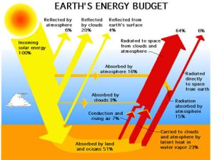
The Earth’s Energy Budget represents the balance between the Sun’s incoming energy and the Earth’s outgoing energy. [1] [2] This budget is crucial for regulating the temperature of the planet. In many ways, the Earth’s Energy Budget works like any budget; to stay balanced, the amount coming in must match the amount going out. Its like a bank account – if you withdraw the same amount of money you deposit, the account balance will remain the same. Your balance will increase if you put more money into your account than you take out. In the case of the Earth’s Energy Budget, the incoming energy from the Sun needs to equal the outgoing energy from the Earth for Earth’s temperature to stay the same – if less goes back out to space than comes in, the temperature increases. [3]
A limited number of things can alter the energy balance of the entire planet. The following are key factors that can impact the global energy balance:
- Greenhouse gases (heat-trapping gases)
- Volcanic Eruptions
- Changes in the Sun’s energy
- Human activities that add aerosols into the atmosphere
- Changes in land use and land cover
The subsequent chapters will discuss how these factors impact Earth’s Energy Budget and influence climate. This exploration will help us understand how human activities have altered Earth’s climate.
- "What Is Earth’s Energy Budget? Five Questions with a Guy Who Knows." NASA , 16 Aug. 2017, www.nasa.gov/feature/langley/what-is-earth-s-energy-budget-five-questions-with-a-guy-who-knows. Accessed 14 Aug. 2023. ↵
- The Global Climate Observing System (n.d.). Earth Radiation Budget. Retrieved June 29, 2023, from https://gcos.wmo.int/en/essential-climate-variables/earth-radiation#:~:text=The%20Earth%20Radiation%20Budget%20(at,only%20be%20measured%20from%20space. ↵
- NOAA, National Weather Service. "The Earth-Atmosphere Energy Balance." National Weather Service, JetStream, https://www.noaa.gov/jetstream/atmosphere/energy Accessed 5 May 2023. ↵
Energy balance is "the difference between the total incoming and total outgoing energy. If this balance is positive, warming occurs; if it is negative, cooling occurs. Averaged over the globe and over long time periods, this balance must be zero. Because the climate system derives virtually all its energy from the Sun, zero balance implies that, globally, the absorbed solar radiation, that is, incoming solar radiation minus reflected solar radiation at the top of the atmosphere and outgoing longwave radiation emitted by the climate system are equal." (IPCC AR6 Glossary)
When most people say "aerosol," they often refer to a specific type of product that produces an aerosol spray, like hairspray. When you press the nozzle, liquid particles suspended in the gas come out. When scientists talk about aerosols, they refer to a broad category of tiny solid or liquid particles or droplets- a typical size between 0.01 and 10 mm - suspended in a gas, which can occur naturally or be a result of human activities. For example, when you see dust floating in a beam of sunlight you see a natural example of aerosols suspended in the air, while soot from gas powered cars is an example of aerosols from human activities. (See IPCC 2018)
Climate Change Primer Copyright © by Marcella Recher. All Rights Reserved.
Share This Book
| All Time | Past Year | Past 30 Days | |
|---|---|---|---|
| Abstract Views | 0 | 0 | 0 |
| Full Text Views | 25661 | 8884 | 737 |
| PDF Downloads | 22052 | 6038 | 609 |
Related Content
The impacts of interannual climate variability on the declining trend in terrestrial water storage over the tigris–euphrates river basin, evaluation of snowfall retrieval performance of gpm constellation radiometers relative to spaceborne radars, a 440-year reconstruction of heavy precipitation in california from blue oak tree rings, quantifying the role of internal climate variability and its translation from climate variables to hydropower production at basin scale in india, extreme convective rainfall and flooding from winter season extratropical cyclones in the mid-atlantic region of the united states.
- Previous Article
- Next Article
Earth's Global Energy Budget
Displayed acceptance dates for articles published prior to 2023 are approximate to within a week. If needed, exact acceptance dates can be obtained by emailing [email protected] .
- Download PDF
An update is provided on the Earth's global annual mean energy budget in the light of new observations and analyses. In 1997, Kiehl and Trenberth provided a review of past estimates and performed a number of radiative computations to better establish the role of clouds and various greenhouse gases in the overall radiative energy flows, with top-of-atmosphere (TOA) values constrained by Earth Radiation Budget Experiment values from 1985 to 1989, when the TOA values were approximately in balance. The Clouds and the Earth's Radiant Energy System (CERES) measurements from March 2000 to May 2004 are used at TOA but adjusted to an estimated imbalance from the enhanced greenhouse effect of 0.9 W m −2 . Revised estimates of surface turbulent fluxes are made based on various sources. The partitioning of solar radiation in the atmosphere is based in part on the International Satellite Cloud Climatology Project (ISCCP) FD computations that utilize the global ISCCP cloud data every 3 h, and also accounts for increased atmospheric absorption by water vapor and aerosols.
Surface upward longwave radiation is adjusted to account for spatial and temporal variability. A lack of closure in the energy balance at the surface is accommodated by making modest changes to surface fluxes, with the downward longwave radiation as the main residual to ensure a balance.
Values are also presented for the land and ocean domains that include a net transport of energy from ocean to land of 2.2 petawatts (PW) of which 3.2 PW is from moisture (latent energy) transport, while net dry static energy transport is from land to ocean. Evaluations of atmospheric reanalyses reveal substantial biases.
National Center for Atmospheric Research, * Boulder, Colorado
* The National Center for Atmospheric Research is sponsored by the National Science Foundation
AMS Publications
Get Involved with AMS
Affiliate sites.
Email : [email protected]
Phone : 617-227-2425
Fax : 617-742-8718
Headquarters:
45 Beacon Street
Boston, MA 02108-3693
1200 New York Ave NW
Washington, DC 200005-3928
- Privacy Policy & Disclaimer
- Get Adobe Acrobat Reader
- © 2024 American Meteorological Society
- [81.177.180.204]
- 81.177.180.204
Character limit 500 /500
Feature | March 25, 2021
Direct observations confirm that humans are throwing earth's energy budget off balance.

A NASA supercomputer model shows how greenhouse gases like carbon dioxide (CO 2 ) – a key driver of global warming – fluctuate in Earth’s atmosphere throughout the year. Higher concentrations are shown in red. Credit: NASA’s Scientific Visualization Studio / NASA’s Global Modeling and Assimilation Office.
By Sofie Bates, NASA’s Earth Science News Team
A NASA study has confirmed with direct evidence that human activities are changing Earth's energy budget, trapping much more energy from the Sun than is escaping back into space.
Earth is on a budget – an energy budget . Our planet is constantly trying to balance the flow of energy in and out of Earth’s system. But human activities are throwing that off balance, causing our planet to warm in response.
Radiative energy enters Earth’s system from the sunlight that shines on our planet. Some of this energy reflects off of Earth’s surface or atmosphere back into space. The rest gets absorbed, heats the planet, and is then emitted as thermal radiative energy the same way that black asphalt gets hot and radiates heat on a sunny day. Eventually this energy also heads toward space, but some of it gets re-absorbed by clouds and greenhouse gases in the atmosphere. The absorbed energy may also be emitted back toward Earth, where it will warm the surface even more.
Adding more components that absorb radiation – like greenhouse gases – or removing those that reflect it – like aerosols – throws off Earth’s energy balance and causes more energy to be absorbed by Earth instead of escaping into space. This is called a radiative forcing, and it’s the dominant way human activities are affecting the climate.
Get NASA's Climate Change News: Subscribe to the Newsletter »
Climate modelling predicts that human activities are causing the release of greenhouse gases and aerosols that are affecting Earth’s energy budget. Now, a NASA study has confirmed these predictions with direct observations for the first time: radiative forcings are increasing due to human actions, affecting the planet’s energy balance and ultimately causing climate change. The paper was published online on March 25, 2021, in the journal Geophysical Research Letters.
“This is the first calculation of the total radiative forcing of Earth using global observations, accounting for the effects of aerosols and greenhouse gases,” said Ryan Kramer, first author on the paper and a researcher at NASA’s Goddard Space Flight Center in Greenbelt, Maryland, and the University of Maryland, Baltimore County. “It’s direct evidence that human activities are causing changes to Earth’s energy budget.”
NASA’s Clouds and the Earth’s Radiant Energy System (CERES) project studies the flow of radiation at the top of Earth’s atmosphere. A series of CERES instruments have continuously flown on satellites since 1997. Each measures how much energy enters Earth’s system and how much leaves, giving the overall net change in radiation. That data, in combination with other data sources such as ocean heat measurements, shows that there’s an energy imbalance on our planet.
“But it doesn’t tell us what factors are causing changes in the energy balance,” said Kramer.

This study used a new technique to parse out how much of the total energy change is caused by humans. The researchers calculated how much of the imbalance was caused by fluctuations in factors that are often naturally occurring, such as water vapor, clouds, temperature, and surface albedo (essentially the brightness or reflectivity of Earth’s surface). For example, the Atmospheric Infrared Sounder (AIRS) instrument on NASA’s Aqua satellite measures water vapor in Earth’s atmosphere. Water vapor absorbs energy in the form of heat, so changes in water vapor will affect how much energy ultimately leaves Earth’s system. The researchers calculated the energy change caused by each of these natural factors, then subtracted the values from the total. The portion leftover is the radiative forcing.
The team found that human activities have caused the radiative forcing on Earth to increase by about 0.5 Watts per square meter from 2003 to 2018. The increase is mostly from greenhouse gases emissions from things like power generation, transport and industrial manufacturing. Reduced reflective aerosols are also contributing to the imbalance.
The new technique is computationally faster than previous model-based methods, allowing researchers to monitor radiative forcing in almost real time. The method could be used to track how human emissions are affecting the climate, monitor how well various mitigation efforts are working, and evaluate models to predict future changes to the climate.
“Creating a direct record of radiative forcing calculated from observations will allow us to evaluate how well climate models can simulate these forcings,” said Gavin Schmidt, director of NASA’s Goddard Institute of Space Studies (GISS) in New York City. “This will allow us to make more confident projections about how the climate will change in the future.”
Related Stories
Earth’s Global Energy Budget Essay
- To find inspiration for your paper and overcome writer’s block
- As a source of information (ensure proper referencing)
- As a template for you assignment
Sources of Earth’s Energy
Earth’ energy imbalance and implications, causes of global warming, principles of remote sensing, remote sensing, works cited.
Earth’s Global energy Budget is an article written by Kevin Trenberth, John Fasullo, and Jeffery Kiehi. This article dwells on various issues related to earth’s energy budget. It also focuses on the sources of earth’s energy and various methods used to measure it (Trenberth, Fasullo, and Kiehl 1).
Earth’s climate is determined by the quantity and distribution of ration from the sun. A stable climate is usually achieved when outgoing longwave radiation (OLR) regulates incoming absorbed solar radiation (ASR). Inward bound radiant energy is usually absorbed by the earth’s atmosphere.
The shortwave energy (radiant solar) is converted into kinetic energy, potential energy and latent energy before is it released as longwave radiant energy (Trenberth, Fasullo, and Kiehl 1). Energy may be transported in different forms, stored for a short period or transformed into the different types, thus creating different types of climate on earth’s surface. In addition, the energy balance can be altered in several ways adjusting earth’s climate and weather (Trenberth, Fasullo, and Kiehl 1).
Modern technology is currently being used to estimate and analyze earth’s energy budget. Some experts have used satellite data to document earth’s energy budget for the annual cycle and inter-annual changeability. Several new measurements have been done, especially from CERES (clouds and the earth’s radiant energy system) devices on a number of platforms.
In addition, there are several new estimates made about earth’s energy budget that are credible. Several examinations on the content of ocean heat have also provided a comprehensive analysis of the global heat balance (Trenberth, Fasullo, and Kiehl 2).
For example, Trenberth, Fasullo, and Kiehl present an evaluation of the earth’s energy budgets at the surface and Top of atmosphere (TOA) for the global ambiance, land surface and ocean on the basis of ocean temperature estimates, land domain simulations and analysis of data retrieved from satellite (2). They limited the TOA budget to correspond to estimates of the global disparity during latest periods of satellite coverage related to adjustments in climate and atmospheric composition (Trenberth, Fasullo, and Kiehl 2).
They also analyze the ocean heat budget in great detail and provide observable estimates of energy deviation and a complete evaluation of uncertainty. By discretely examining the land and ocean spheres, Trenberth, Fasullo, and Kiehl discovered a setback in the previous alteration made to Earth Radiation Budget Experiment data when NOAA-9 fail and found it appropriate to harmonize the record independently over land and ocean rather than on a global basis.
The outcome was a modified and somewhat better value for the global outgoing longwave radiation than in KT97. Nonetheless, even larger adjustments emerged from using CERES data that apparently reveal better precision of CERES retrievals and its accuracies in retrieval method as well as its utilization of Moderate Resolution Imaging Spectroradiometer technology for scene recognition (Trenberth, Fasullo, and Kiehl 2).
The discussions above have outlined some of the key issues and problems associated with determining earth’s energy budget. It is appropriate to inspect the ocean and land spheres independently so as to take advantage of the limitations that arises with them and particularly to the capability of the land and ocean to store energy.
According to the article Earth’ Energy Imbalance and Implications, human beings are potentially susceptible to changes in global temperature. Although climate change is caused by several environmental agents, there is a general concession that the current trend in global warming is as a result of human activities that have altered atmospheric composition (Hansen, Sato and Kharecha 1).
The greenhouse effect is basically the major cause of global warming. For example, when the level of carbon dioxide rises, the atmosphere becomes denser at infrared wavelengths. A denser atmosphere causes the earth’s heat radiation in space to emerge from high and colder regions of the atmosphere thereby preventing heat energy to escape to space. The short-term imbalance between the heat energy absorbed by the atmosphere and heat energy released to space causes the earth to warm until planetary energy equilibrium is re-established.
A climate forcing is defined by planetary energy discrepancy attributed to an adjustment of atmospheric composition. Climate sensitivity, defined as the ultimate change of global temperature per unit forcing, is a well-known phenomenon. However, there are two key elements that constrain the ability of humans to predict changes in global temperatures on a long-term basis (Hansen, Sato and Kharecha 1).
The first element is climate forcing brought about by man-made aerosol which is virtually immeasurable. Aerosols are fine elements; such as sulfates, dust and black soot, suspended in the air. Aerosol climate forcing is intricate since aerosols both absorb solar radiation (which increases temperatures) and reflect solar radiation to space (causing temperatures to fall).
Moreover, atmospheric aerosol can change cloud properties and cloud cover. Second, the rate at which the temperature of the earth’s surface moves toward stability in reaction to a climatic forcing is determined by the manner in which heat perturbations are efficiently blended into the ocean (Hansen, Sato and Kharecha 2).
Climate sensitivity is determined by climate feedbacks- which entail numerous physical processes that arise when climate adjusts in reaction to a forcing. Positive (magnifying) feedbacks raise the climate response whereas negative (weakening) feedbacks decrease the response. Climate problem are mainly caused climate feedbacks.
Climate feedbacks are complex phenomena to grasp because a climate forcing can be wrongly interpreted as a climate feedback and vice versa. Climate models- developed on the basis of physical laws that portray the dynamics and structure of the land processes, ocean and atmosphere- are utilized to simulate climate. These models help climate experts to grasp the nature of climate sensitivity since they can alter processes in the climate model and examine their interactions (Hansen, Sato and Kharecha 4).
As noted above, global warming is mainly caused by human activities. However, there are several environmental factors that contribute to changes in global temperature. Greenhouse gases such as carbon dioxide increases the density of the atmosphere which in turn prevents heat radiation from escaping to space. This phenomenon leads to global warming. In addition, humans are unable to analyze the underlying cause of global warming because of the complicated nature of climate feedbacks (Hansen, Sato and Kharecha 4).
According to the article Principles of Remote Sensing written by Aggarwal, remote sensing is a method used to monitor atmosphere or earth’s surface using satellite technology or airplanes (23). Several aspects of electromagnetic field are used in remote sensing. It captures data on electromagnetic energy reflected by the surface of earth. The quantity of radiation from radiance (object) is determined by both radiation striking the radiance and the property of the object (Aggarwal 23).
Remote sensing refers to the indirect process of acquiring information about objects found on earth’s surface. Humans use sensing instruments to measure electromagnetic energy transmitted by an object.
Remote sensing instruments enable humans to capture images of earth’s surface in different wavelength areas of electromagnetic spectrum (EMS). A number of of the pictures symbolize reflected solar radiation in the observable infrared areas of the EMS whereas others measure the amount of energy released by the surface of earth (Aggarwal 24).
Remote sensing is essentially a multifaceted science discipline which entails an amalgamation of several disciplines for example photography, spectroscopy, electronic, telecommunication and computer. These disciplines are combined to form a complete system called Remote Sensing System.
There are several phases in a remote sensing process: discharge of electromagnetic radiation (EMR); transmission of energy from the source to earth’s domain; interface of electromagnetic radiation with the surface of earth; broadcast of energy from earth’s surface to the remote sensor; and output of sensor data (Aggarwal 24).
The radiation from the sun is either reflected by earth’s surface, conveyed into the surface or emitted by earth’s surface. On interaction, the electromagnetic radiation experiences several adjustments in direction, magnitude, polarization, phase and wavelength. These adjustments are registered by the remote sensor and the interpreter is able to retrieve vital data concerning the object under observation. The data retrieved has spectral information (color, spectral mark and tone) and spatial data-direction, shape and size (Aggarwal 30).
As noted above, the main source of radiation and electromagnetic radiation is the sun. Radiation from the sun is usually reflected by earth’s surface and sensed by airplane-borne sensor or satellite. The interaction between the atmosphere and electromagnetic radiation is critical to remote sensing for two key purposes.
First, the interactions of electromagnetic with atmosphere enable interpreters to acquire important information concerning the atmosphere itself. Second, data conveyed by electromagnetic radiation is adjusted while navigating via the atmosphere. The atmospheric elements disperse and soak up the radiation reflected from the object by altering its spatial allotment. Both absorption and scattering differ with respect to their effect from one end of the spectrum to another (Aggarwal 34).
Atmospheric scattering takes place when electromagnetic radiations are redirected by fine particles suspended in the atmosphere. Scattering not only alters the spectral signature of objects but also decreases the contrast of the image.
The quantity of electromagnetic radiation scattered is determined by a number of factors: the wavelength of EMR; the mass of particles; the volume of particles; and the density of the atmosphere. The concentration of these particles fluctuates depending on the season and time. This implies that the outcomes of scattering will be spatially irregular and will differ from one season to another (Aggarwal 35).
As noted above, the sun is the main source of EMR. Remote sensing refers to the indirect process of acquiring information about objects found on earth’s surface. Humans use different sensing instruments to measure electromagnetic energy transmitted by an object. The quantity of radiation from an object is determined by both radiation striking the radiance and the property of the object. Remote sensing is thus a useful technique for identifying and classifying various features of the earth and atmosphere.
Aggarwal, Shefali. Principle of Remote Sensing . Dehra Dun: Indian Institute of Remote Sensing, n.d. Print.
Hansen, James, Sato Makiko, and Kharecha, Pushker. Earth’s energy Imbalance and Implications . New York: Columbia University Earth Institute, 2010. Print.
Trenberth, Kevin, Fasullo John, and Kiehl, Jeffery . Earth’s Global Energy Budge t. Boulder, Colorado: National Center for Atmospheric Research, 2008. Print.
- Remote Sensing and Geographical Information System for Developing Countries
- Narrow Band Sensor and Wide Band Sensor in Engines
- Researching Capacitive Touch Sensor
- The Temperate Forest Biome's Greatest Sustainability Threats
- Climate Shift Could Leave Some Marine Species Homeless
- Nuclear Power Advantages and Disadvantages
- Ecosphere Care in the United States
- Mitigation Plan for Energy Resources
- Chicago (A-D)
- Chicago (N-B)
IvyPanda. (2018, October 19). Earth’s Global Energy Budget. https://ivypanda.com/essays/earths-global-energy-budget/
"Earth’s Global Energy Budget." IvyPanda , 19 Oct. 2018, ivypanda.com/essays/earths-global-energy-budget/.
IvyPanda . (2018) 'Earth’s Global Energy Budget'. 19 October.
IvyPanda . 2018. "Earth’s Global Energy Budget." October 19, 2018. https://ivypanda.com/essays/earths-global-energy-budget/.
1. IvyPanda . "Earth’s Global Energy Budget." October 19, 2018. https://ivypanda.com/essays/earths-global-energy-budget/.
Bibliography
IvyPanda . "Earth’s Global Energy Budget." October 19, 2018. https://ivypanda.com/essays/earths-global-energy-budget/.
Earth's Energy Budget Diagram

Scientists have been able to document global incoming and outgoing radiation averages, which provide an understanding of how energy is absorbed, reflected, and released by Earth's atmosphere, clouds, and surface. The numbers in parentheses represent the uncertainty range, or variability, associated with these averages.
IPCC, WG1, 2021
The upper panel of the image shows a schematic representation of Earth’s energy budget for the early 21st century, including globally averaged estimates of the individual components, in units Watts per square meter (W m -2 ). The image also shows the uncertainty or variability ranges (5-95% confidence), represented by the numbers in parentheses. The lower panel shows the energy budget in the absence of clouds, with otherwise identical atmospheric and surface properties. Without clouds, less solar radiation is reflected back to space globally (53 ± 2 W m –2 instead of 100 ± 2 W m –2 ), and overall more thermal radiation is emitted from Earth's surface and atmosphere back to space. The difference in how much incoming solar radiation reaches Earth's surface means the planet would warm substantially if there were no clouds.
Thank you for visiting nature.com. You are using a browser version with limited support for CSS. To obtain the best experience, we recommend you use a more up to date browser (or turn off compatibility mode in Internet Explorer). In the meantime, to ensure continued support, we are displaying the site without styles and JavaScript.
- View all journals
- Explore content
- About the journal
- Publish with us
- Sign up for alerts
- Correspondence
- Published: 19 May 2013
Energy budget constraints on climate response
- Alexander Otto 1 ,
- Friederike E. L. Otto 1 ,
- Olivier Boucher 2 ,
- John Church 3 ,
- Gabi Hegerl 4 ,
- Piers M. Forster 5 ,
- Nathan P. Gillett 6 ,
- Jonathan Gregory 7 ,
- Gregory C. Johnson 8 ,
- Reto Knutti 9 ,
- Nicholas Lewis 10 ,
- Ulrike Lohmann 9 ,
- Jochem Marotzke 11 ,
- Gunnar Myhre 12 ,
- Drew Shindell 13 ,
- Bjorn Stevens 11 &
- Myles R. Allen 1 , 14
Nature Geoscience volume 6 , pages 415–416 ( 2013 ) Cite this article
16k Accesses
233 Citations
450 Altmetric
Metrics details
- Climate change
To the Editor
The rate of global mean warming has been lower over the past decade than previously. It has been argued 1 , 2 , 3 , 4 , 5 that this observation might require a downwards revision of estimates of equilibrium climate sensitivity, that is, the long-term (equilibrium) temperature response to a doubling of atmospheric CO 2 concentrations. Using up-to-date data on radiative forcing, global mean surface temperature and total heat uptake in the Earth system, we find that the global energy budget 6 implies a range of values for the equilibrium climate sensitivity that is in agreement with earlier estimates, within the limits of uncertainty. The energy budget of the most recent decade does, however, indicate a lower range of values for the more policy-relevant 7 transient climate response (the temperature increase at the point of doubling of the atmospheric CO 2 concentration following a linear ramp of increasing greenhouse gas forcing) than the range obtained by either analysing the energy budget of earlier decades or current climate model simulations 8 .
This is a preview of subscription content, access via your institution
Relevant articles
Open Access articles citing this article.
Crucial role of sea surface temperature warming patterns in near-term high-impact weather and climate projection
- & Thomas Knutson
npj Climate and Atmospheric Science Open Access 13 June 2024
Solar cycle as a distinct line of evidence constraining Earth’s transient climate response
- King-Fai Li
- & Ka-Kit Tung
Nature Communications Open Access 19 December 2023
Quantifying the cooling effect of tropical cyclone clouds on the climate system
- , Elizabeth A. Ritchie
- & J. Scott Tyo
npj Climate and Atmospheric Science Open Access 24 July 2023
Access options
Subscribe to this journal
Receive 12 print issues and online access
251,40 € per year
only 20,95 € per issue
Buy this article
- Purchase on Springer Link
- Instant access to full article PDF
Prices may be subject to local taxes which are calculated during checkout
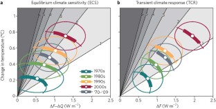
Aldrin, M. et al. Environmetrics 23 , 253–271 (2012).
Article Google Scholar
Lewis, N. J. Clim. http://dx.doi.org/10.1175/JCLI-D-12-00473.1 (2013).
Ring, M. J., Lindner, D., Cross, E. F. & Schlesinger, M. E. Atmos. Clim. Sci. 2 , 401–415 (2012).
Google Scholar
Stott, P. A., Good, P., Jones, G., Gillett, N. P. & Hawkins, E. Environ. Res. Lett. 8 , 014024 (2013).
Schwartz, S. E. Surv. Geophys. 33 , 745–777 (2012).
Gregory, J. M. & Forster, P. M. J. Geophys. Res. Atmos. 113 , D23105 (2008).
Allen, M. R. & Frame, D. J. Science 318 , 582–583 (2007).
Taylor, K. E., Stouffer, R. J. & Meehl, G. A. Bull. Am. Meteorol. Soc. 93 , 485–498 (2011).
Morice, C., Kennedy, J. J., Rayner, N. A. & Jones, P. D. J. Geophys. Res. http://dx.doi.org/10.1029/2011JD017187 (2013).
Forster, P. M. et al. J. Geophys. Res. Atmos. 118 , 1–12 (2013).
Vial, J., Dufresne, J-L. & Bony, S. Clim. Dynam. http://dx.doi.org/10.1007/s00382-013-1725-9 (2013).
Held, I. M. et al. J. Clim. 23 , 2418–2427 (2010).
Armour, K. C., Bitz, C. M. & Roe, G. H. J. Clim. http://dx.doi.org/10.1175/JCLI-D-12–00544.1 (2012).
Gregory, J. M., Stouffer, R. J., Raper, S. C. B., Stott, P. A. & Rayner, N. A. J. Clim. 15 , 3117–3121 (2002)..
Gillett, N. P., Arora, V. K., Matthews, D. & Allen, M. R. J. Clim. http://dx.doi.org/10.1175/JCLI-D-12-00476.1 (2013).
Frame, D. J. et al. Geophys. Res. Lett. 32 , L09702 (2005).
Download references
Author information
Authors and affiliations.
Environmental Change Institute, University of Oxford, South Parks Road, Oxford, OX1 3QY, UK
Alexander Otto, Friederike E. L. Otto & Myles R. Allen
Laboratoire de Météorologie Dynamique, IPSL/CNRS, UPMC, Paris, France
Olivier Boucher
CSIRO Marine and Atmospheric Research Hobart, Castray Esplanade, Hobart Tasmani, 7000, Australia
John Church
Grant Institute, University of Edinburgh, West Mains Road, Edinburgh, EH9 3JW, UK
Gabi Hegerl
School of Earth and Environment, University of Leeds, Leeds, LS2 9JT, UK
Piers M. Forster
Canadian Centre for Climate Modelling and Analysis, PO Box 3065 STNCSC, Victoria, British Columbia, Canada
Nathan P. Gillett
Department of Meteorology, University of Reading, PO Box 243, Reading, RG6 6BB, UK
Jonathan Gregory
NOAA/Pacific Marine Environmental Laboratory, 7600 Sand Point Way NE, Seattle, 98115, Washington, USA
Gregory C. Johnson
Institute for Atmospheric and Climate Science, ETH Zurich, Zurich, 8092, Switzerland
Reto Knutti & Ulrike Lohmann
Walden, Widcombe Hill, Bath, BA2 6ED, UK
Nicholas Lewis
Max Planck Institute for Meteorology, Bundesstraße 53, Hamburg, D-20146, Germany
Jochem Marotzke & Bjorn Stevens
CICERO, P.O. Box 1129 Blindern, Oslo, N-0318, Norway
Gunnar Myhre
NASA Goddard Institute for Space Studies, 2880 Broadway, New York, 10025, New York, USA
Drew Shindell
Department of Physics, University of Oxford, Parks Road, Oxford, OX1 3PU, UK
Myles R. Allen
You can also search for this author in PubMed Google Scholar
Contributions
O.B., J.C., G.H., P.F., N.P.G., J.G., G.C.J., R.K., N.L., U.L., J.M., G.M., D.S., B.S., and M.R.A. conceived the analysis and designed the headline figure. P.M.F. provided the forcing data and estimates. G.C.J. provided the heat content data. A.O. conducted the analysis and produced the figures. A.O., F.E.L.O., M.R.A., P.M.F., O.B., and G.C.J contributed to writing the paper.
Corresponding author
Correspondence to Alexander Otto .
Ethics declarations
Competing interests.
The authors declare no competing financial interests.
Supplementary information
Supplementary information (original).
Supplementary information (original) (PDF 970 kb)
Supplementary information (corrected)
Supplementary information (corrected) (PDF 570 kb)
Rights and permissions
Reprints and permissions
About this article
Cite this article.
Otto, A., Otto, F., Boucher, O. et al. Energy budget constraints on climate response. Nature Geosci 6 , 415–416 (2013). https://doi.org/10.1038/ngeo1836
Download citation
Published : 19 May 2013
Issue Date : June 2013
DOI : https://doi.org/10.1038/ngeo1836
Share this article
Anyone you share the following link with will be able to read this content:
Sorry, a shareable link is not currently available for this article.
Provided by the Springer Nature SharedIt content-sharing initiative
This article is cited by
- Thomas Knutson
npj Climate and Atmospheric Science (2024)
Theoretical tools for understanding the climate crisis from Hasselmann’s programme and beyond
- Valerio Lucarini
- Mickaël D. Chekroun
Nature Reviews Physics (2023)
Time-variations of the climate feedback parameter λ are associated with the Pacific Decadal Oscillation
- Benoît Meyssignac
- Jonathan Chenal
- Aurélien Ribes
Communications Earth & Environment (2023)
- Elizabeth A. Ritchie
- J. Scott Tyo
npj Climate and Atmospheric Science (2023)
- Ka-Kit Tung
Nature Communications (2023)
Quick links
- Explore articles by subject
- Guide to authors
- Editorial policies
Sign up for the Nature Briefing newsletter — what matters in science, free to your inbox daily.

Information
- Author Services
Initiatives
You are accessing a machine-readable page. In order to be human-readable, please install an RSS reader.
All articles published by MDPI are made immediately available worldwide under an open access license. No special permission is required to reuse all or part of the article published by MDPI, including figures and tables. For articles published under an open access Creative Common CC BY license, any part of the article may be reused without permission provided that the original article is clearly cited. For more information, please refer to https://www.mdpi.com/openaccess .
Feature papers represent the most advanced research with significant potential for high impact in the field. A Feature Paper should be a substantial original Article that involves several techniques or approaches, provides an outlook for future research directions and describes possible research applications.
Feature papers are submitted upon individual invitation or recommendation by the scientific editors and must receive positive feedback from the reviewers.
Editor’s Choice articles are based on recommendations by the scientific editors of MDPI journals from around the world. Editors select a small number of articles recently published in the journal that they believe will be particularly interesting to readers, or important in the respective research area. The aim is to provide a snapshot of some of the most exciting work published in the various research areas of the journal.
Original Submission Date Received: .
- Active Journals
- Find a Journal
- Proceedings Series
- For Authors
- For Reviewers
- For Editors
- For Librarians
- For Publishers
- For Societies
- For Conference Organizers
- Open Access Policy
- Institutional Open Access Program
- Special Issues Guidelines
- Editorial Process
- Research and Publication Ethics
- Article Processing Charges
- Testimonials
- Preprints.org
- SciProfiles
- Encyclopedia
Journal Menu
- Atmosphere Home
- Aims & Scope
- Editorial Board
- Reviewer Board
- Topical Advisory Panel
- Instructions for Authors
- Special Issues
- Sections & Collections
- Article Processing Charge
- Indexing & Archiving
- Editor’s Choice Articles
- Most Cited & Viewed
- Journal Statistics
- Journal History
- Journal Awards
- Society Collaborations
- Editorial Office
Journal Browser
- arrow_forward_ios Forthcoming issue arrow_forward_ios Current issue
- Vol. 15 (2024)
- Vol. 14 (2023)
- Vol. 13 (2022)
- Vol. 12 (2021)
- Vol. 11 (2020)
- Vol. 10 (2019)
- Vol. 9 (2018)
- Vol. 8 (2017)
- Vol. 7 (2016)
- Vol. 6 (2015)
- Vol. 5 (2014)
- Vol. 4 (2013)
- Vol. 3 (2012)
- Vol. 2 (2011)
- Vol. 1 (2010)
Find support for a specific problem in the support section of our website.
Please let us know what you think of our products and services.
Visit our dedicated information section to learn more about MDPI.
Earth System Energy Budget and Climate Change
- Print Special Issue Flyer
- Special Issue Editors
Special Issue Information
- Published Papers
A special issue of Atmosphere (ISSN 2073-4433). This special issue belongs to the section " Climatology ".
Deadline for manuscript submissions: closed (31 January 2023) | Viewed by 1789
Share This Special Issue
Special issue editor.

Dear Colleagues,
The energy budget imbalance of the Earth system is closely linked to climate change, and the net energy input will warm the system. The interactions between components of the climate system will redistribute the energy tempospatially. Although great progress has been achieved in the quantitative calculations of the energy budget and energy transports in the climate system, there are still large uncertainties and discrepancies between observations, numerical simulations, and re-analyses. Therefore, we are pleased to organize this Special Issue entitled “Earth System Energy Budget and Climate Change”.
Papers related to the following areas are welcome:
- Radiative fluxes at the top of the atmosphere;
- Energy accumulation and transport in the atmosphere;
- Surface heat fluxes;
- Heat storage and transport in the oceans;
- Energy budget imbalances in the Earth system;
- Direct and indirect validations of the energy fluxes;
- Consistency between observations and numerical simulations;
- Physical processes related to energy change, storage, and transport;
- Interactions between different scales.
Prof. Dr. Chunlei Liu Guest Editor
Manuscripts should be submitted online at www.mdpi.com by registering and logging in to this website . Once you are registered, click here to go to the submission form . Manuscripts can be submitted until the deadline. All submissions that pass pre-check are peer-reviewed. Accepted papers will be published continuously in the journal (as soon as accepted) and will be listed together on the special issue website. Research articles, review articles as well as short communications are invited. For planned papers, a title and short abstract (about 100 words) can be sent to the Editorial Office for announcement on this website.
Submitted manuscripts should not have been published previously, nor be under consideration for publication elsewhere (except conference proceedings papers). All manuscripts are thoroughly refereed through a single-blind peer-review process. A guide for authors and other relevant information for submission of manuscripts is available on the Instructions for Authors page. Atmosphere is an international peer-reviewed open access monthly journal published by MDPI.
Please visit the Instructions for Authors page before submitting a manuscript. The Article Processing Charge (APC) for publication in this open access journal is 2400 CHF (Swiss Francs). Submitted papers should be well formatted and use good English. Authors may use MDPI's English editing service prior to publication or during author revisions.
- energy budget
- energy transport
- climate change
- physical processes
- observations
- numerical simulations
Published Papers (1 paper)
Further Information
Mdpi initiatives, follow mdpi.
Subscribe to receive issue release notifications and newsletters from MDPI journals

45,000+ students realised their study abroad dream with us. Take the first step today
Meet top uk universities from the comfort of your home, here’s your new year gift, one app for all your, study abroad needs, start your journey, track your progress, grow with the community and so much more.

Verification Code
An OTP has been sent to your registered mobile no. Please verify

Thanks for your comment !
Our team will review it before it's shown to our readers.
- School Education /
Save Energy Essay in 500+ Words in English

- Updated on
- Jun 13, 2024

‘When the sun is bright, say no to tube light’. I know this sounds more like a nursery rhyme but trust me, it is the cheat code to save energy for a sustainable future. Today, the annual global energy conservation is 580 million terajoules, and do you know where we get the most of this energy? The sun and Earth’s natural resources. Governments and NGOs across the world are organising climate and energy conservation summits to raise awareness and implement sustainable energy guidelines. Today, our Save Energy essay will guide you towards this modern approach to energy conservation and how do we achieve it.

Table of Contents
- 1 Why Should We Save Energy?
- 2 How Can We Save Energy?
- 3 Conclusion
- 4 Save Energy Essay 200 words
Why Should We Save Energy?
In the words of Jimmy Carter, one of the most admired former U.S. presidents, ¨Because we are now running out of gas and oil, we must prepare quickly for a third change, to strict conservation and to the use of… Permanent renewable energy sources, like solar power
The world of today needs more important resources. Among those, energy is one of the most important ones therefore it is crucial to save energy for many reasons, impacting our environment and daily lives.
As of 2024, global energy consumption is rising continuously and is putting strain on natural resources and the issues related to the environment. As per IEA (International Energy Agency), energy demand has increased by an average of 3.4 percent annually through 2026. It should be noted there was a rise in consumption from 18 percent in 2015 to 20 percent in 2023.
One of the primary reasons to save energy is to reduce greenhouse gas emissions. Efficient consumption of energy via solar PV and wind generation for the years 2021 to 2022 helped around 465 Mt of Carbon Dioxide emissions in the power sector.
Without cleaning energy technologies which further included eclectic vehicles, and other heat pumps saving 85 Mt Carbon Dioxide would not be possible.
Additionally, saving energy helps in leading economic benefits too. Practising energy-efficiency practices and technologies helps at ground level to save energy. Moreover, conservation of energy ensures the longer life of non-renewable resources such as fossil fuels, coal, oil, and natural gas.
In conclusion, saving energy helps not only protect our environment but also reduce the costs of consumption which further leads to a sustainable future. Small changes in our daily activities can contribute to a greener and more energy-efficient world.
Quick Read: Essay on Global Warming
How Can We Save Energy?
We all know that energy conservation helps not only reduce greenhouse gas emissions but also promote sustainable development. Now the question is, how can we save energy at ground level? So here are some simple but effective ways to save energy:
1. At Home:
- Practice turning off lights and appliances when they are not in use.
- Replace the more energy-consuming bulbs with energy-efficient LED bulbs.
- It is advisable to adjust the temperature of the air-conditioner accordingly.
- Do not forget to unplug the electronics and charge them when not in use. Practice using energy-efficient appliances and equipment, which also make efficient use of energy.
2. At School:
- Peers should be made aware of ” The Car Pooling” practice. Also, the use of public transportation should be boosted.
- Children should be encouraged to use energy carefully. The practice of energy-saving habits such as turning off computers and other electronic devices when not in use should be taught.
- Regularly setting up energy-saving campaigns and competitions can also help raise awareness about saving energy.
- Special classes should be given to promote and install solar panels or other renewable energy sources.
Government initiatives and policies such as the Energy Conservation Building Code (ECBC), the Perform, Achieve and Trade (PAT) flagship programme of the Bureau of Energy under the National Mission for Enhanced Energy Efficiency (NMEEE), Jawaharlal Nehru National Solar Mission (JNNSM) and many more are notable examples that are led by the government for the sustainability of energy.
Saving energy is not a sole activity; instead, it is a collective responsibility that needs the active participation of individuals, communities, businesses and governments. By adopting the correct practices of saving energy in our daily lives, we can contribute to a greener way of life and a brighter future for ourselves as well as for future generations.
Also Read: Essay on Indian Farmers in 100, 200, and 350 words
Save Energy Essay 200 words
How would it be if you had superpowers that could help your school, community, and the planet Earth? Isn’t that exactly what happens when you become an “ Energy-saving superhero? ” It might seem small, but if you trust in helping hands, tiny habits like turning off a computer and other gadgets can add up to a big difference.
As a student, the first and foremost mission to save energy begins in the classroom. Are the lights left on in empty rooms? Are fans and other electrical equipment functioning without any purpose and constantly draining energy? Become a “Detective of Power” and turn off every purposeless appliance that sucks up energy.
Next, unleash your inner “ Eco-Warrior .” To accomplish this purpose, ensure that all electronic items are switched off when everyone is leaving, as every watt saved is a miraculous victory for the planet. Shortening bathroom breaks, taking shorter showers, and using an air dryer only when needed are other super ways to save water and energy, and of course, to finally use the power of nature.
By becoming an “ Energy Superhero ,” we will not only help our school and other important places but also save money on electricity bills. Be a responsible citizen, grab your cape, and let your mission to save energy begin.
Also Read: Short and Long Essay on National Memorial Day
Ans: 10 ways to save energy include the following: a) Turn off lights when leaving a room. b) Unplug chargers and electronics when not in use. c) Use energy-efficient LED bulbs. d) Set air conditioners at moderate temperatures. e) Take shorter showers to save hot water. f) Wash clothes in cold water whenever possible. g) Use a clothesline instead of a dryer. h) Carpool or use public transportation. i) Properly insulate your home. j) Purchase energy-efficient appliances.
Ans: Saving energy means using less energy or consuming the energy efficiently. The saving of energy includes the necessary steps that reduce the amount of energy that we waste in our daily lives, at home, school or at work.
Ans: Energy powers our homes, schools, and workplaces. We need energy to run appliances, lights, and electronics. Energy fuels transportation like cars, buses, and trains. Industries require energy to operate machines and equipment. Energy helps us cook food and heat or cool our buildings.
Discover some interesting topics in Essay Writing
For more information on such interesting topics, visit our essay writing page and follow Leverage Edu .

Deepika Joshi
Deepika Joshi is an experienced content writer with expertise in creating educational and informative content. She has a year of experience writing content for speeches, essays, NCERT, study abroad and EdTech SaaS. Her strengths lie in conducting thorough research and ananlysis to provide accurate and up-to-date information to readers. She enjoys staying updated on new skills and knowledge, particulary in education domain. In her free time, she loves to read articles, and blogs with related to her field to further expand her expertise. In personal life, she loves creative writing and aspire to connect with innovative people who have fresh ideas to offer.
Leave a Reply Cancel reply
Save my name, email, and website in this browser for the next time I comment.
Contact no. *

Connect With Us
45,000+ students realised their study abroad dream with us. take the first step today..

Resend OTP in
Need help with?
Study abroad.
UK, Canada, US & More
IELTS, GRE, GMAT & More
Scholarship, Loans & Forex
Country Preference
New Zealand
Which English test are you planning to take?
Which academic test are you planning to take.
Not Sure yet
When are you planning to take the exam?
Already booked my exam slot
Within 2 Months
Want to learn about the test
Which Degree do you wish to pursue?
When do you want to start studying abroad.
January 2024
September 2024
What is your budget to study abroad?

How would you describe this article ?
Please rate this article
We would like to hear more.
Have something on your mind?

Make your study abroad dream a reality in January 2022 with
India's Biggest Virtual University Fair

Essex Direct Admission Day
Why attend .

Don't Miss Out
Issue Brief | Obama FY2016 Budget Proposal: Sustainable Energy, Buildings, Transportation & Climate
February 4, 2015
On February 2, 2015, President Obama released his $4 trillion fiscal year (FY) 2016 budget proposal for the federal government. The request includes $563 billion for non-defense discretionary spending – $5 billion over FY 2015 enacted levels. The budget reflects the administration's "all of the above" energy strategy, as well as its continued focus on addressing climate change and investing in infrastructure. The proposed 2016 budget increases the Department of Energy’s (DOE) funding by 9 percent over 2014 enacted levels, raises the Environmental Protection Agency's (EPA) budget by 5.5 percent, and hikes the Department of Transportation’s (DOT) funding by 31 percent.
The proposal invests $7.4 billion in clean energy technology programs across all agencies , led by DOE, the Department of Defense (DOD), the National Science Foundation (NSF), and the Department of Agriculture (USDA). Other highlights include a proposed $4 billion Clean Power Plan Incentive Fund to encourage states to go beyond their minimum carbon reduction requirements, as well as $1.29 billion for the Global Climate Change Initiative (GCCI), which supports multilateral and bilateral international efforts to combat climate change. Transportation programs include a new $7.5 billion Critical Immediate Investments Program and a $7.4 billion increase for the Federal Transit Administration (a 67 percent increase).
This issue brief outlines the Obama administration’s FY 2016 budget request for several clean energy and infrastructure programs within key agencies.
DEPARTMENT OF ENERGY
The President’s FY 2016 budget request for the Department of Energy (DOE) is $29.9 billion, an increase of 9 percent over FY 2015 enacted levels, compared to an overall federal budget increase of 3.6 percent. The proposed budget is built to further the Administration’s all-of-the-above energy strategy and its Climate Action Plan, announced June 2013. The White House aims to reduce domestic greenhouse gas emissions 17 percent by 2020, 26-28 percent by 2025 and 83 percent by 2050, all with respect to 2005 levels. To this end, the White House’s budget request focuses on DOE’s role in transitioning to a low carbon economy through a more resilient, economical, and clean energy system.
The 2016 request increases the Office of Energy Efficiency and Renewable Energy (EERE) budget 42 percent over 2015 enacted levels , to $2.7 billion. The Office of Electricity Delivery and Energy Reliability would grow nearly 84 percent to $270 million, with a 133 percent increase in funding for energy infrastructure resiliency , a 94 percent increase for smart grid R&D , and a 75 percent increase for energy storage . The Office of Fossil Energy would grow by 6.4 percent to $842 million. The Office of Nuclear Energy's budget would increase 8.9 percent to $907 million. The DOE Office of Science, which funds basic research in the physical sciences, will grow 5.4 percent to $5.3 billion. The budget also provides $325 million for the Advanced Research Projects Agency – Energy (ARPA-E), an increase of 16 percent. ARPA-E funds the development of innovative energy technologies that show promise but are not ready for market investment. In keeping with its multi-year open solicitation policy, ARPA-E does not plan to release an open solicitation in 2016. However, ARPA-E will provide seven to ten technology funding opportunities throughout the year, and continue its Small Business Innovation Research/Small Business Technology Transfer program.
The budget request funds five crosscutting initiatives which are conducted in partnership between the three Under Secretariats of DOE: Science and Energy, Nuclear Security, and Management and Performance. The initiatives are funded within DOE’s programs. They include work on grid modernization, supercritical carbon dioxide (sCO2)-based power generation, subsurface engineering, the energy-water nexus, and cybersecurity.
This year DOE will start a new loan guarantee program for tribal energy, at a level of $11 million. This money will be used to leverage private funding for energy projects on tribal lands.
The President’s FY 2016 Energy Efficiency and Renewable Energy budget request for DOE includes:
- A 44 percent increase in funding for the Solar Energy program to nearly $336 million , to help the SunShot Initiative achieve its goal of a solar energy price of $0.06/kWh, without subsidies.
- A 36 percent increase in funding for the Wind Energy program to $145 million , which will support three advanced offshore wind demonstration projects, planned to begin power generation in 2017. DOE is also supporting an Atmosphere to Electrons initiative to lower the cost of wind energy and enhance wind farm performance.
- A nearly 10 percent increase in funding for the Water Power program to $67 million , to fund a new initiative called HydroNEXT, which will research and develop ways to increase hydropower on pre-existing dams, water conveyance systems, and streams. HydroNEXT will also research cheap modular systems with small environmental and construction footprints, as well as marine and hydrokinetic technologies.
- A 75 percent increase in funding for the Geothermal Technologies program to $96 million , to fully implement the Subsurface Technology and Engineering RD&D crosscut, an effort to decrease the risks and costs of geothermal development by using lessons learned in other subsurface sectors. The funding also supports the Frontier Observatory for Research in Geothermal Energy (FORGE), a site to test innovative geothermal technologies.
- A 6 percent increase in funding for the Hydrogen and Fuel Cell Technologies program to $103 million , which will focus on technologies and materials that will reduce hydrogen production, compression, transport, and storage costs. Funding will also provide resources to rapidly advance the development of quality control tools for the manufacturing of fuel cell components and systems.
- A 59 percent increase in funding for the Vehicle Technologies program to $444 million , to support greater investment in vehicle electrification and grid infrastructure, improved freight hauling efficiency, and partnerships to demonstrate community-scale alternative fuel vehicles. The program will continue to work toward aspirational vehicle technology goals, such as improving battery energy storage.
- An over 9 percent increase for the Bioenergy Technologies program to $246 million , to develop advanced cellulosic and algal-based gasoline, jet and diesel fuel at a price of $3 per gallon gasoline equivalent (gge). The budget will also fund commercial-scale demonstration biorefineries to make fuel for the military, in partnership with the Departments of Navy and Agriculture.
- A 31 percent increase for the Weatherization and Intergovernmental Assistance Program to $318 million , to fund low-income weatherization services for about 33,000 homes in FY 2016 and the State Energy Program, which will also help government facilities and operations share best practices to decrease their annual energy use 2 percent by 2020.
- A 59 percent increase in funding for the Federal Energy Management program to $43 million , with a new $15 million investment to help federal agencies meet energy efficiency and renewable energy requirements.
- A 102 percent increase for the Advanced Manufacturing program to $404 million , which will fully fund two new Clean Energy Manufacturing Innovation Institutes, while continuing funding for the four existing institutes. These institutes will be part of an interagency National Network of Manufacturing Institutes, focused on convening universities, companies, and the government to solve industry problems and improve U.S. competitiveness.
- A 53 percent increase in funding for the Building Technologies program to $264 million , to support advanced materials and technologies R&D, appliance standards development, and other initiatives to reduce building energy use.
DOE crosscutting initiatives showcase an overlay of priorities which elaborates on the funding levels above. The following table shows which DOE programs are supporting the crosscutting initiatives, and at what level.
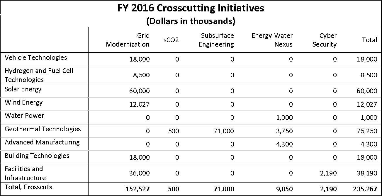
USDA / DOE BIOENERGY PROGRAMS
Department of energy bioenergy programs.
The Bioenergy Technologies Program is part of DOE’s Sustainable Transportation initiative within the Office of Energy Efficiency and Renewable Energy. The FY 2016 budget proposes funding of $246 million, an increase of 9.3 percent above the FY 2015 appropriated level. Similar to FY2015, the budget emphasizes "development of innovative processes to convert cellulosic and algal-based feedstocks to bio-based gasoline, jet and diesel fuels at a cost of $3.00 per gallon gasoline equivalent." The Department of Energy is continuing its collaboration with the U.S. Department of Agriculture and the U.S. Navy to demonstrate commercial-scale biorefineries to produce military-specification fuels, as well as supporting development of new technologies that are still in the research stage.
Within the Bioenergy Technologies program, $38.8 million is requested for feedstocks development and pre-pilot scale logistics, an increase of $6.8 million over FY15 enacted levels. Of this, $21 million is for advancing algae feedstocks , and $17.8 million is allocated to cellulosic feedstocks .
U.S. Department of Agriculture (USDA) Bioenergy & Sustainable Farms and Forests Programs
FY 2014 and early 2015 have seen the roll-out of many energy efficiency, renewable energy and conservation programs established under the Agricultural Act of 2014 (Farm Bill). President Obama’s budget request for energy title programs for FY 2016 is $32 million higher than FY 2015 funding levels. The Farm Bill contains robust mandatory funding for its Energy Title Programs over its five-year authorization.
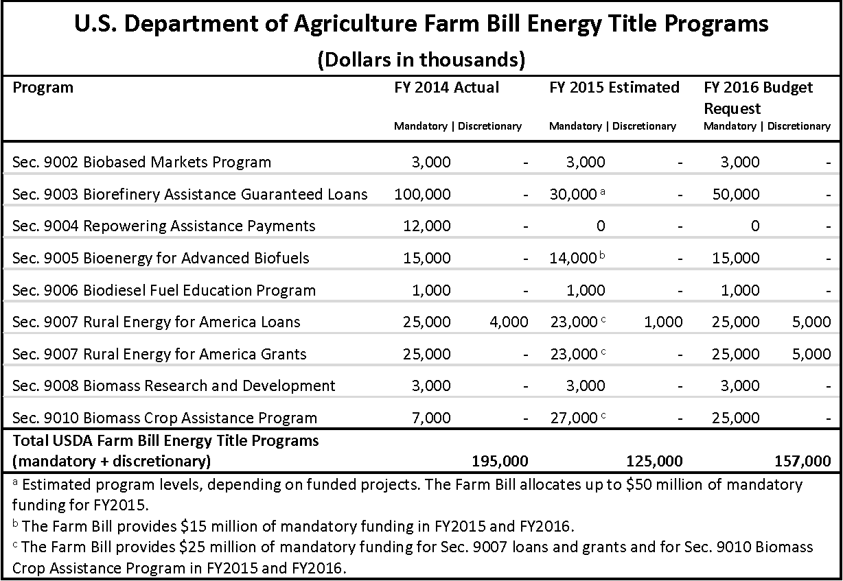
Additionally, the President’s FY 2016 USDA budget request includes several new programs, as well as stable or increased funding levels for existing programs that will continue to put farms, forests and rural economies on a more sustainable path. Climate change and its impact on water availability, extreme weather events as well as the growing climate-water-agricultural nexus received increased attention and funding throughout the budget request. Conservation and related programs include:
- First floated in the President’s 2015 Budget proposal, the President continues to advocate for “treating catastrophic fire as a natural disaster” through the creation of a separate $855 million emergency disaster fund . According to USDA, fire suppression has grown from “13 percent of the agency’s budget in the 1990s to over 50 percent in 2014.” As fire-related costs have soared, the practice of ‘fire transfer’ has increased, which redirects essential funds from other programs to fighting wildfires.
- 2015 support levels are maintained for local sustainable forest initiatives under Integrated Resource Restoration (IRR) at $822 million, and the Collaborative Forest Landscape Restoration Program (CFLRP) at $60 million. These programs will decrease the number of catastrophic wildfires by funding restoration practices that reduce hazardous fuels as well as help restore water quality, and increase carbon sequestration.
- Total funding of 2016 Farm Bill conservation programs is $6.3 billion . This includes conservation programs at both the Forest Service (FS) and the Natural Resources Conservation Service (NRCS). USDA estimates an additional 7 million acres will be enrolled per year under the Conservation Stewardship Program and will continue to support 24 million acres enrolled under the Conservation Reserve Program.
- A $125 million increase of the Agriculture and Food Research Initiative (AFRI) relative to FY15 funding levels, to $450 million for FY16. Research areas include the role of water supply and availability to agricultural and food production.
- Additionally, under the Agricultural Research Service (ARS), environmental stewardship programs will receive $206 million . This includes funding to continue the Regional Hubs for Risk Adaptation and Mitigation to Climate Change.
- The Economic Research Service will receive $1 million to study the impacts of climate change on the water-agriculture-food nexus.
- Provision of $200 million for Watershed and Flood Prevention Operations , which assists communities and land owners in becoming more resilient to climate change.
- The proposed budget includes $10 million in funding over two years for USDA and other agencies to study the effects of incentives and outreach on farmer adoption of conservation practices , in order to foster conservation programs that are the least-cost option.
ENERGY-EFFICIENT / SUSTAINABLE BUILDINGS PROGRAMS
Department of energy.
The DOE’s Building Technologies Office seeks to develop and promote technologies and practices that will reduce U.S. building energy consumption by 50 percent from the 2010 Annual Energy Outlook baseline. According to the Energy Information Agency (EIA), residential and commercial buildings across the country consumed more than 40 percent of total U.S. energy (and more than 73 percent of U.S. electricity) in 2013. America’s energy bill of more than $430 billion could be cost effectively reduced 20-50 percent if available solutions were applied and new products and practices were successfully developed and commercialized. In recognition of the building sector’s importance, the DOE buildings program benefits from a substantial 53 percent increase in proposed funding over 2015 enacted levels.
The FY 2016 request of $264 million for Building Technologies emphasizes R&D for lighting, building envelopes, and heating and cooling; facilitates the development of minimum energy efficiency requirements; and supports activities to improve the efficiency and resiliency of the electric grid and its connections to buildings and related infrastructure. The budget request also supports a new R&D effort for advanced building envelope and refrigerant materials manufacturing; assists home owners and builders in adopting energy efficiency solutions; and provides new resources and tools to the commercial sector with a goal of achieving a 20 percent reduction in energy use by 2020. Energy conservation standards and test procedures directly support national energy policy objectives, such as increasing energy savings and energy productivity, and reducing carbon emissions.
Building Technologies programs and public-private partnerships focus on individual building components as well as system-design strategies and tools that integrate and optimize components into high-performing, low-energy systems. The Building Technologies Office also provides technical assistance and training; education and outreach; technical review of model building energy codes; support to the states and local jurisdictions that adopt and enforce such codes; and development of appliance and equipment standards. These initiatives help the building industry apply new technologies and practices cost-competitively; provide consumers with the knowledge to demand better houses and buildings; and ensure that buildings are safe, durable and affordable.
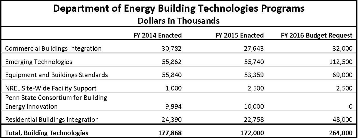
Department of Housing and Urban Development (HUD)
HUD’s FY 2016 budget proposes $49.3 billion in budget authority, an increase of more than 8 percent over FY 2015 levels . The budget emphasizes the Department’s core commitment to provide Americans with access to affordable housing, but also seeks to continue helping communities "prepare for the risks posed by extreme weather and other natural disasters, while strengthening communities' ability to be economically resilient in the face of a changing climate and natural disasters."
Energy efficiency also factors into the HUD budget. HUD spends between $4 and $6 billion per year on energy for its public housing stock. Reducing those expenditures would be a win for HUD and the Public Housing Authorities that own and operate public housing and a win for the environment by reducing greenhouse gas emissions associated with fossil-fuel generated energy. The FY 2016 budget therefore continues funding for the Energy Performance Contracting (EPC) program and proposes a Utilities Conservation Pilot that would encourage Public Housing Authorities (PHAs) of all sizes to undertake needed energy conservation measures.
The administration is also proposing $4.6 billion for the Public Housing Operating Fund , a $160 million increase over the 2015 enacted level. HUD is proposing a change in policy for public housing construction and operation that has the potential to dramatically reduce energy use and operational costs in the HUD portfolio. The change would allow PHAs with more than 250 public housing units to use their operating reserves for capital expenditures. This would provide a powerful incentive to conserve operating expenses, such as energy use.
With regards to climate change adaptation , HUD has allocated $14.2 billion of the $15.2 billion it received to respond to Hurricane Sandy. The remaining $1 billion is earmarked for the Office of Economic Resiliency's National Disaster Resilience Competition , which will be awarded in FY2016. Also included is a Pay for Success demonstration that allows HUD to enter multiyear agreements to repay private investors who provide upfront funding for energy efficiency retrofits of HUD-assisted housing.
HUD maintains and updates a federal building code for manufactured housing (24 CFR Part 3282), a type of U.S. factory-built housing that is an important source of affordable housing. Since the HUD Code came out in 1976, the fire safety, durability and quality of manufactured homes have greatly improved. Further code changes that will greatly increase the energy efficiency of manufactured housing are anticipated.
HUD is requesting $50 million for the Policy Development and Research (PD&R) Research and Technology (R&T) account for fiscal year 2016, $22 million less than the 2015 appropriation. PD&R is responsible for providing research on building technology, disaster housing (which FEMA provides to communities), resilient housing and resilient communities. This request will fully fund PD&R’s housing surveys, including the American Housing Survey, and continue research dissemination functions.
DEPARTMENT OF TRANSPORTATION
The proposed Department of Transportation (DOT) FY 2016 budget requests a total of $94.7 billion in mandatory and discretionary funds, a 31 percent increase from an estimated $72.1 billion in 2015. The recent extension of the MAP-21 surface transportation authorization expires on May 31, 2015, so the budget includes a six-year surface transportation reauthorization proposal which would fund a Transportation Trust Fund (TTF) with $240 billion from federal fuels taxes and other existing revenue sources, supplemented with $238 billion from a 14 percent mandatory tax on $2 trillion of existing corporate earnings held overseas. The new TTF would include the current Highway Trust Fund’s highway and mass transit accounts, and add rail and multimodal accounts. The proposal would increase funding for the Federal Highway Administration (FHWA) by $10.4 billion, the Federal Transit Administration (FTA) by $7.4 billion, the Federal Railroad Administration (FRA) by $3.4 billion, and National Infrastructure Investment (TIGER) grants by $750 million.

The proposed FTA budget ($18.4 billion) would reduce transit’s $86 billion maintenance backlog and avoid increased congestion costs as urban populations continue to grow . Formula grants ($13.9 billion) would increase 160 percent for rail and 350 percent for bus. Capital Investment Grants ($3.25 billion) would increase by $1.13 billion, with 28 New/Small Starts and Core Capacity projects in 15 states. There would be a new grant program for Rapid Growth Area Transit focused on Bus Rapid Transit ($500 million). Another new competitive grant program, Fixing and Accelerating Surface Transportation (FAST), would provide $500 million to the FTA, and another $500 million to the FHWA, for innovative State and local solutions to pressing transportation performance challenges.
The FHWA budget ($51.3 billion) contains a new Freight Program ($1 billion) to incentivize regional, multi-modal projects, and a new $7.5 billion Critical Immediate Investments Program (“Fix-it-First”) to reduce the number of structurally deficient Interstate Highway bridges . Otherwise, the program structure established under MAP-21 continues. The $10.3 billion Surface Transportation Program provides flexible (mode) funding for states to work with Metropolitan Planning Organizations (MPO) or local transportation officials in rural areas. The Congestion Mitigation and Air Quality (CMAQ) Improvement program ($2.3 billion) provides flexible funds for state and local governments to reduce regional congestion and meet air quality standards (NAAQS). The Transportation Alternatives Program ($847 million) helps create livable communities, and the Metropolitan Transportation Planning Program ($320 million) supports MPOs’ multi-modal planning. The $1 billion Transportation Infrastructure Finance and Innovation Act (TIFIA) program subsidizes loans for projects of national or regional significance, facilitates private participation and leverages up to $30 billion in investment. New bond programs also encourage private investment (i.e. America Fast Forward, Qualified Public Infrastructure Bonds).
The FRA budget ($5 billion) contains a new Current Passenger Rail Service program which subsumes Amtrak programs and increases funding by $1 billion, to return public rail assets to a state of good repair and make critical investments to maintain current services . Program areas include: Northeast Corridor ($550 million), State Corridors ($225 million), Long Distance ($850 million), National Assets, Debt and PTC ($475 million) and Stations ($350 million). A new Rail Service Improvement Program ($2.3 billion) expands and improves rail networks. It includes Passenger Corridors ($1.3 billion) to develop new or improve existing corridors, Commuter Railroad PTC ($825 million) for safety (due to sunset FY18), Local Rail Facilities and Safety ($125 million) and Planning and Workforce ($75 million). The Safety and Operations program would expand to address safety issues related to energy product movement, passenger rail and highway-rail crossings.
The $166 million Research, Engineering and Development program in the FAA budget request maintains $6 million to support continuing efforts to partner with industry to transition general aviation off leaded fuel , and $24 million for aircraft technologies to increase efficiency and reduce harmful emissions by advancing alternative jet fuels.
In the budget for the Office of the Secretary, the TIGER multimodal grant program (National Infrastructure Investment) would increase by 150 percent . The Interagency Permitting Improvement Center proposal is carried over from last year’s request, to continue implementation of coordinating concurrent (rather than serial) interagency project reviews.
The Army Corps of Engineers budget requests $915 million from the Harbor Maintenance Trust Fund , to help the nation’s ports prepare for larger cargo vessels. This amount is 16 percent less than 2015 funding, and below the $1.32 billion target set by the recently passed authorization law (WRRDA).
Please see the Department of Energy budget analysis regarding Vehicle and Bioenergy/alternate fuels programs.
ENVIRONMENTAL PROTECTION AGENCY
The President’s FY 2016 budget request for the Environmental Protection Agency (EPA) is $8.6 billion, an increase of $452 million (5.5 percent) from FY 2015 enacted funding. Funds for addressing climate change and improving air quality amount to $1.11 billion, an increase of $120 million (12 percent) from FY 2015. The $1.1 billion request includes $214 million to support the Clean Power Plan and other regulatory and partnership programs to reduce climate change pollution domestically and abroad. Separately from the $8.6 billion requested for FY 2016, the Administration is proposing to create the Clean Power Plan Incentive Fund, which would provide states with as much as $4 billion for going beyond the minimum requirements of the Clean Power Plan.
The EPA breaks down its budget request into five overall goals. Two of those five goals address climate change and sustainable communities, and are highlighted below.
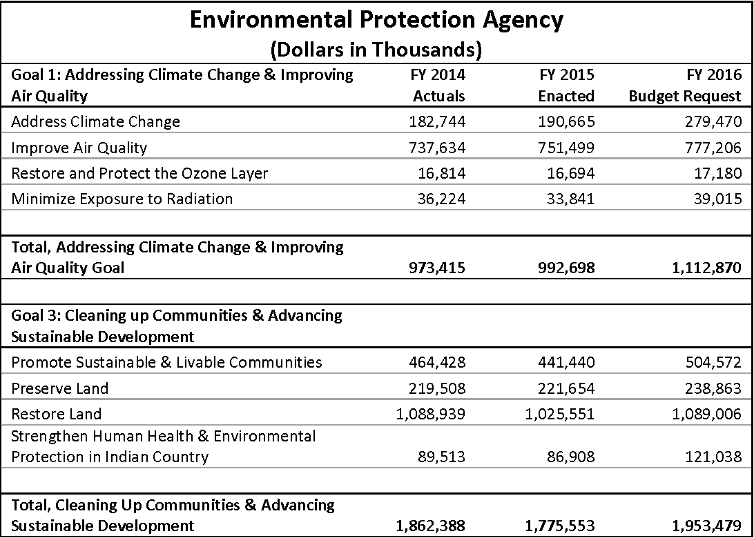
The FY 2016 EPA budget request also includes:
- $25 million for grants to states to develop their strategies for the Clean Power Plan
- $5 million for climate resilience grants through the Wetlands Program Development Grants program
- $4 million increase over current levels for the ENERGY STAR program
- $14 million for the Environmental Justice program, a 107 percent increase over FY 2015. It incorporates the concerns of disproportionately impacted minority, low-income and tribal communities into rulemaking.
DEPARTMENT OF STATE
The Department of State’s FY 2016 budget request includes $1.29 billion for the Global Climate Change Initiative (GCCI) , which supports international organizations that facilitate climate change resilience and affordable renewable energy in developing nations. This includes $549 million in multilateral assistance for international climate and clean energy efforts , with $150 million for the Green Climate Fund, $168 million for the Global Environment Facility (GEF), $171 million for the Clean Technology Fund (CTF), and $60 million for the Strategic Climate Fund (SCF). The Strategic Climate Fund includes funding for three programs: the Pilot Program for Climate Resilience (PPCR), the Forest Investment Program (FIP), and the Program for Scaling up Renewable Energy in Low-Income Countries (SREP).
The Global Climate Change Initiative budget request also includes $306 million in bilateral development assistance for climate adaptation, clean energy, and the sustainable landscapes program . The remaining portion of the GCCI request is $448 million for the Oceans and International Environmental and Scientific Affairs (OES) program, which supports, among other programs, the Clean Energy Ministerial, the U.S.-Africa Clean Energy Finance initiative, and the international Climate and Clean Air Coalition. Of the $448 million in OES funds, $350 million would go to the Green Climate Fund, which is to receive $500 million in all in 2016 . The Obama administration has promised $3 billion in total for the Fund, to be paid out over four years.
OTHER AGENCY HIGHLIGHTS
The Department of Commerce's $9.8 billion budget request includes $6.18 billion in budget authority for the National Oceanic and Atmospheric Administration (NOAA), up $511 million from FY 2015. The request includes $2.38 billion for the National Environmental Satellite, Data, and Information Service (NESDIS), which will be used to improve weather predictions and modeling. The agency has requested $507 million for NOAA’s Office of Oceanic and Atmospheric Research (OAR), which includes $160 million for climate research (a 22 percent increase over FY 2015). The NOAA budget request includes $50 million for its Regional Coastal Resilience Grant program.
The Department of Defense (DOD) budget provides support for energy efficiency initiatives, including improving fuel efficiency, developing new energy technologies, and expanding renewable energy resources . The Energy Conservation Investment Program (ECIP), which supports renewable energy and energy efficiency projects at military installations, remains at the FY 2015 appropriations level of $150 million. The budget request for the Operational Energy Capability Improvement fund is $37 million, down $9 million from FY 2015 funding levels. The budget request includes $48 million for the Navy Energy Program, $16 million lower than FY 2015.
The Department of Interior (DOI) budget request for renewable energy initiatives is $100 million, an increase of $8 million above FY 2015 enacted levels . The renewable funding request includes $34 million for the Bureau of Ocean Management, $29 million for the Bureau of Land Management, $14 million for the Fish and Wildlife Service, and $9 million for the Bureau of Indian Affairs. DOI also requests $195 million for climate adaptation activities, including $50 million for planning and technical assistance to communities and tribes.
The Department of Homeland Security (DHS) budget request for the Federal Emergency Management Agency (FEMA) includes $200 million for its Pre-disaster Mitigation Grant Program, an eight-fold increase over current funding. The FEMA request also includes $279 million for the Flood Hazard Mapping and Risk Analysis program, a $194 million increase over FY 2015.
Create an account
Create a free IEA account to download our reports or subcribe to a paid service.
- Tracking COP28 Progress
- United States
- Latin America and the Caribbean
- European Union
- Middle East
- Japan and Korea
- Southeast Asia
Cite report
IEA (2024), World Energy Investment 2024 , IEA, Paris https://www.iea.org/reports/world-energy-investment-2024, Licence: CC BY 4.0
Share this report
- Share on Twitter Twitter
- Share on Facebook Facebook
- Share on LinkedIn LinkedIn
- Share on Email Email
- Share on Print Print
Report options
Past and future energy investment in africa in the announced pledges scenario and in the net zero emissions by 2050 scenario, 2016-2030, burdened by significant debt repayments, financing for clean energy projects is scarce as the need for concessional support becomes increasingly evident.
Achieving Africa’s energy- and climate-related goals by 2030 will require annual investments of over USD 200 billion through the end of this decade. This will be vital to meet the growing energy needs of a continent where the median age of the population is 20 years and average GDP per capita is just over one-fourth of the global average.
Our tracking of energy spending suggests that around USD 110 billion is set to be invested in energy across Africa in 2024, of which nearly USD 70 billion to fossil fuel supply and power, with the remainder going to a range of clean energy technologies. Spending trends vary widely across Africa, but neither the total amount nor the proportion spent on clean energy are enough to put the continent on track to reach its sustainable development goals. As they stand, energy investments are equivalent to only 1.2% of the region’s GDP and clean energy investments, while rising, account for just 2% of the global total.
Debt repayments, which have increased sharply in recent years, mean that many African governments have difficulty accessing the funds required for capital-intensive clean energy projects. Moreover, low sovereign debt ratings further limit access to outside investment – in 2023, only two countries, Botswana and Mauritius, held investment-grade ratings.
Of the clean energy investments that have recently been made, the majority are in renewable power generation. While these projects are vital to meet Africa’s rising electricity needs in a sustainable way, the prospects for further growth will be limited as long as the grid itself is not upgraded and expanded. With average line losses of 15%, inefficient grids and insufficient interconnections are already creating bottlenecks for new renewable energy projects in the region.
Energy access is among the top priorities in Africa, where 600 million people live without electricity and roughly 1 billion people lack access to clean cooking. Financing needs for energy access initiatives fall well short of the annual USD 25 billion that is required to achieve the 2030 objectives of full access to modern energy. Progress in this area will require concessional finance providers to mobilise grants for the most vulnerable households and support the creation of bankable projects. The provision of other derisking capital will also be critical to allow the private sector to take a more active role.
A high cost of capital is a major impediment to scaling up clean energy investments in Africa. Reducing country-wide and project-specific risks will require a major effort from national policymakers, based on clear strategies and ambitious NDCs, alongside significantly more international financial and technical support.
Subscription successful
Thank you for subscribing. You can unsubscribe at any time by clicking the link at the bottom of any IEA newsletter.
Overview: Our plan for New South Wales
Nsw snapshot, budget repair that puts people first, budget highlights.
- 1. Building a better New South Wales
- 1.1 Housing and planning
- 1.2 Building homes for NSW
- 1.3 Transport
- 1.4 Roads
- 1.5 Health
- 1.6 Education
- 1.7 Better protection for victim-survivors of domestic and family violence
- 1.8 Better support for our community
- 1.9 Our regions, energy and environment
- 1.10 Supporting businesses and protecting consumers
- 1.11 Disaster relief and recovery
- 1.12 Building better communities
- 1.13 Cost of living relief
Building a better NSW
In the 15 months since the people of NSW elected this Government, much has been done, and much remains to do. This, our second budget – only 9 months since the first – continues our focus on the vision we have and the work needed to realise it:
- the work still to be done for the millions of families and businesses burdened by decades-high levels of inflation
- the duty we still owe to the tens-of-thousands of patients who turn to our public hospitals for urgent care
- the task of providing hundreds of thousands of students attending our public schools with a world-leading education
- the responsibility we have to protect every community against crime, tragedy and terror
- and the job we have lifted from the too-hard basket: to back every citizen striving to own a home, rent a home, or who needs social housing.
These challenges are this Government’s causes. We do not expect to overcome them in a single budget. But in each Labor budget, we will make progress. When we pair the public’s resources with the people’s priorities, real change can happen.
In this Labor budget we continue our plans to bust the wages cap, reform tolls, back first-home buyers, build new and better public schools and hospitals, speed up the renewables revolution, rebuild rural and regional roads, help small businesses, and wrangle debt back under control.
But still, more progress is possible
Careful management of the public’s finances means we can afford to accelerate change.
We can do more to prevent family and domestic violence. And we can do more to support victim-survivors.
We can do more to help people visit their GP. And we can surge more resources into our emergency departments.
And for housing
We can change planning laws and incentivise councils to build more homes close to infrastructure and services.
We can build homes for key workers to rent in the places we need them to be.
And we can restore social housing so that it is once again a reliable foothold for people who find themselves able to rely on so little else.
These things are essential for the better NSW the Minns Labor Government is determined to build.
This budget continues our plan to make this vision a reality.

The Hon. Daniel Mookhey MLC NSW Treasurer
Population by area

Population by age

Share of owner occupied dwellings
Source: Australian Bureau of Statistics, 2021 Census
public hospitals
surgeries performed
emergency and non-emergency incidents responded to by NSW Ambulance
Emergency services
Fire and Rescue NSW firefighters
fire stations
Rural Fire Service volunteers
State Emergency Service volunteers
police officers
operational police stations
calls for service
public schools
existing public preschools
services per week
train lines
average daily services
ferry routes
Source: NSW Government. Data reflects the most recent 12 month period available. Time periods may vary.
Electricity generation
NSW electricity generation for consumption (TWhs)

Source: NSW Government
Families and business remain burdened by historically high inflation and a housing crisis
The people of NSW are doing it tough. After years of bushfires, floods and a global pandemic, high inflation and rising interest rates have left households and businesses under pressure.
Nowhere is this pressure felt more acutely than for housing. NSW has the highest mortgages of any state in the country and bears the greatest burden as interest rates rise.
In times of crisis, we realise what matters most. At a time of escalating costs, families need to know that the essential services we rely on are there to support us.
Budget repair over the past 12 months
15 months ago, the new Government was presented with a budget shortfall of $7.0 billion . The Government’s comprehensive review of expenditure reigned in ballooning expense growth for 2023-24 and beyond.
In our first budget, this Government also took significant steps to stabilise the State’s gross debt levels, suspending NSW Generations Fund (NGF) contributions in 2023-24, reforming the Transport Asset Holding Entity (TAHE), and saving more than $13.0 billion through the Comprehensive Expenditure Review.
By taking this action to stabilise our fiscal position and lower our debt, the Government was able to begin sustainable repair of our essential services and offer targeted support to help with housing, energy, tolls and healthcare – where people are feeling the most pressure.
Gross debt saving since Pre-election Budget Update (PEBU)

Source: NSW Treasury
Budget result before and after Commonwealth Grants Commission (CGC GST) reduction

Early signs of progress
In our first year, the NSW Government has made progress.
- 2,100 more nurses have been hired.
- Since announcing paid study for police recruits, there has been more than a 40 per cent increase in applications compared to the same period last year.
- There has been a 20 per cent fall in teacher vacancies, the beginning of the Government’s efforts to reduce teacher vacancies and lost learning in NSW public schools.
These are early signs that our approach to re-building our essential services is working. Our investments in safe staffing levels, pay for police recruits, new salary scales across the teaching profession and the abolition of the wages cap are already improving our health system, frontline policing and public schools.
While we have begun to make progress, we still have much to do to build a better NSW.
The GST rip-off
As we undertake this work, we must manage the fall out of having billions stripped out of the Budget by the Commonwealth Grants Commission’s 2024 GST decision.
The CGC’s decision in March to cut GST payments to NSW will cost our budget $11.9 billion over the next four years. The decision has taken more revenue from NSW than was lost in the COVID-19 pandemic.
A long-term plan for a better NSW
The 2024-25 Budget reflects the Government’s calm and methodical response to the unexpected shock of the Commonwealth’s GST decision. We will not sell off public assets or continue the past practice of undermining essential services by further suppressing wages.
The Government’s long-term plan remains to control expenses and reign in debt, to sustainably rebuild essential services. The unexpected downgrade of $11.9 billion Commonwealth revenue will stretch our resources for the foreseeable future. It means our path to recovery will be slower, but this Government will not pass on to the people of NSW the $11.9 billion hit from the CGC.
Expense outlook

We can afford to make that choice because of the action we have taken – and continue to take – to stabilise the State’s gross debt trajectory. Gross debt was set to rise to $188.2 billion by June 2026 according to the 2022-23 Pre-Election Budget Update. Now, gross debt will be $9.3 billion lower by that time, even after absorbing the GST hit.
While we continue to reduce growth in debt and borrowings, the Government has had to redouble efforts to stabilise our operating position in the face of this new challenge. The projected deficit of $3.6 billion in 2024-25 will gradually reduce to a deficit of $1.5 billion in 2027-28.
From 2018-19 to 2022-23 the average growth of government expenses was 9.7 per cent. In this Budget, total general government sector expenses are projected to increase by an average rate of 1.7 per cent per year from 2023-24 to 2027-28.
While the road to repair will be slower than first thought, the deficit will fall by $6.0 billion between 2023-24 and 2024-25. In 2024-25, the Budget year, we expect to return to cash operating surplus after three years of borrowing to pay our running costs. These are the first steps toward building a better NSW – without privatisation, or an unfair wages cap.
A budget of must-haves
Because we have made careful choices, we can fund the things we need, continue fixing the things that need repair, and fight for our rightful share of Commonwealth revenues.
Our major initiatives include:
- a Bulk-Billing Support Initiative, which includes provision of tax relief to GP practices that meet bulk-billing thresholds
- delivering the homes that a growing city needs – along with health, education and transport infrastructure that communities need to thrive
- funding Western Sydney roads
- extending the Parramatta Light Rail
- building new public schools and funding new school upgrades and maintenance
- upgrading hospitals and health facilities across the State
- delivering record funding for disaster recovery
- expansion of services for mental health and domestic and family violence.
This overview outlines these plans, and more, as we make progress to build a better NSW.This overview outlines these plans, and more, as we make progress to build a better NSW.
to build new public schools and fund school upgrades, and $1.0 billion for maintenance
to upgrade hospitals and health facilities across the State and for key health worker housing across regional and remote NSW
for upgraded roads in Western Sydney, including to the new Western Sydney airport
to build public transport across the State, including three new metro lines, extending the Parramatta Light Rail, and new Western Sydney buses
to build 8,400 social homes, including priority homes for victim-survivors of domestic and family violence
for disaster relief and recovery programs, including $3.3 billion for disaster affected regional roads
to support domestic, family and sexual violence victim-survivors and expand programs that reduce violence against women and children
which includes tax rebates to GP clinics to protect bulk-billing rates
1.1 Housing and planning

Source: Department of Planning, Housing and Infrastructure
More homes where people want to live
The NSW Government is confronting the housing crisis. People need more homes close to transport, infrastructure, other amenities and work opportunities.
The NSW Government has made major reforms to the planning system to build more homes and rebalance housing growth across Sydney, Wollongong, Central Coast and the Hunter.
More homes near better infrastructure
The Transport Oriented Development Program:
- rezones areas around eight train and metro stations as priority precincts for more housing, supported by $520.0 million in new infrastructure
- rezones areas around 37 train and metro stations across greater Sydney to increase midrise housing in well-connected locations.
A better planning system
This Budget invests an additional $555.5 million to speed up the planning system and construct more housing enabling infrastructure. This includes:
- $253.7 million to bolster the State’s planning system, including to assess more development applications and deliver additional State-led rezonings
- $246.7 million for enabling infrastructure, conservation activities and land acquisitions to accelerate the delivery of more housing in Western Sydney and across the regions
- $35.0 million for the NSW Building Commission to support its ongoing efforts to reform the building and construction industry and improve consumer outcomes
- $5.0 million for preliminary design and planning works to support the future redevelopment of Bays West around the Bays Metro station and White Bay Power Station.
Targets and incentives
- We have set new housing targets to rebalance growth towards areas of Sydney with better access to transport and other infrastructure, and share the additional housing Sydney needs across our city.
- This Budget includes $200.0 million for the Faster Assessments program to incentivise councils to meet and exceed their targets by providing grants for infrastructure that supports housing.
1.2 Building homes for NSW
More homes, better rights, building homes for nsw.
To address the housing crisis, the NSW Government will deliver up to 30,000 new homes.
The Building Homes for NSW program will:
- deliver up to 21,000 new market and affordable homes
- build 8,400 social homes, including priority homes for victim-survivors of domestic and family violence
- build more than 500 new rental homes for key workers so they can live in the communities who rely on them.
Building Homes for NSW will directly address the housing crisis alongside our state-wide planning reforms.
Building up to 30,000 new homes
Building Homes for NSW will release surplus Government land for new homes to be delivered by Homes NSW, Landcom and in partnership with the private sector.
The Budget includes $5.0 million to continue the audit of surplus NSW Government land.
A major step to help those escaping from family and domestic violence
This Budget invests $5.1 billion in 8,400 social homes, of which 6,200 will be new homes and 2,200 are replacement homes.
At least 50 per cent of these new homes will be prioritised for victim-survivors of domestic and family violence.
In 2022-23, 18,255 people who sought homelessness services said family and domestic violence was the main reason they needed help, but half were turned away due to a lack of accommodation.
This program also invests $1.0 billion to repair 33,500 existing social homes.
Key worker rental housing
Too many suburbs have become unaffordable for nurses, teachers, police officers, paramedics and other key workers.
The Budget includes $655.1 million for key worker and rental housing:
- $450.0 million for a Key Worker Build-to-Rent Program to be delivered by Landcom across metropolitan areas of the State
- $200.1 million for key health worker accommodation across rural and regional areas of the State
- $5.0 million for Landcom to deliver an additional 10 Build-to-Rent dwellings in Bomaderry, with 60 homes now to be delivered through a total Government investment of $35.0 million .
Better rights
A better system for renters.
This Budget also includes an additional $8.4 million for the Rental Commissioner to develop and enforce renter protections.
Supporting the growing number of renters in apartments with an expanded Strata and Property Services Commissioner to regulate strata schemes for $11.8 million .
Addressing homelessness
$527.6 million for emergency housing and homelessness support services, which includes:
- over $260.0 million to help people and families who need safe shelter with crisis accommodation and support to move to more stable housing
- over $250.0 million of funding to support people who are homeless or at risk of homelessness, including those leaving correctional centres and mental health services and securing funding for Specialist Homelessness Services and the Aboriginal Community Controlled sector for homelessness services.
1.3 Transport
Better transport.
The Government is investing in essential transport infrastructure and technology upgrades to keep our State moving. These essential investments will keep communities connected, support much needed new housing and link people to jobs and opportunities.
Building Parramatta Light Rail 2
The NSW Government has provisioned $2.1 billion for the delivery of Parramatta Light Rail Stage 2 to build better connected communities in Sydney’s growing west. The 2024-25 Budget paves the way to start construction on this essential project.
Sydney Metro
This Budget contains $13.4 billion for the continuation of Sydney Metro West, including the potential for an additional station at Rosehill. This Budget also includes $5.5 billion for the ongoing delivery of the Western Sydney Airport Metro and $1.2 billion funding for the completion of the Sydney Metro City and Southwest.
Building the future of transport
The Tangara fleet will be upgraded and extended for an additional 12 to 15 years, at a cost of $447.0 million .
This extra life span will ensure commuters have safe and reliable public transport while we rebuild our domestic rail manufacturing industry, so we can once again build trains here.
Illawarra Rail Resilience Plan
The Government will fund the $10.0 million Illawarra Rail Resilience Plan to determine options to upgrade and rebuild infrastructure along the South Coast Line following extreme weather events.
Better technology, better journeys
Sydney has a vast and complicated network which is still only partially digitised. This Budget provides:
- $25.0 million for the replacement of the Digital Train Radio System, and
- $40.0 million to expedite technology for train crews during periods of degraded operations and enhance their ability to recover.
Better buses, better services
- $1.9 billion for a new zero emissions bus fleet.
- This Budget provides funding to deliver new dedicated bus services connecting Blacktown, Camden, Campbelltown, Fairfield, Liverpool and Penrith to the new Western Sydney Airport.
- In response to recommendations from the Bus Industry Taskforce, $91.0 million has been allocated to the Bus Transport Management System which will replace the current legacy system and improve real-time information provision to customers.
- The Government is also allocating $23.8 million over two years to develop a state-wide medium-term bus plan.
Better roads for Sydney
Improved arterial roads are needed to support new housing and connect people to jobs and opportunities. This Budget delivers a record investment in Western Sydney roads to connect the Western Sydney Airport to the world and support much needed new housing and jobs.
This Budget allocates $1.0 billion in 2024-25, bringing the total program to $5.2 billion , including matched funding from the Australian Government. The program will:
- upgrade Mamre Road Stage 2 between Erskine Park and Kemps Creek for $1.0 billion
- widen Elizabeth Drive with four lanes connecting Mamre Road and The Northern Road to the airport for $800.0 million
- widen for Richmond Road – M7 to Townson Road for $520.0 million
- upgrade Garfield Road East for $276.3 million
- upgrade Memorial Avenue from Old Windsor Road to Windsor Road for $48.2 million
- add a separated four-lane dual carriageway on Mulgoa Road Stage 2 between Glenmore Park and Jeanette Street for $230.0 million
- upgrade the intersection at St Johns Road and Appin Road for $45.0 million .
Work is underway in partnership with the Australian Government to connect future communities through:
- $65.0 million for South West Sydney Roads Planning
- $30.0 million for Western Sydney Roads Planning
- $25.0 million for Eastern Ring Road and Badgerys Creek Road South
- $15.0 million for Spring Farm Parkway Stage 2 Planning.
Regional communities
Transport networks and roads are critical to life in regional NSW, connecting communities to one another and supporting the movement of goods produced in our regions to national and international markets. This Budget includes significant investment, in partnership with the Australian Government, including:
- $350.0 million for Inland Rail Level Crossings at Parkes and Narrabri
- $275.0 million for Nelson Bay Road to Bob’s Farm
- $130.0 million for the Avoca Drive upgrade
- $105.0 million for Nowra Bypass and Network Planning
- $47.3 million for the Jindabyne Education Campus to provide improved access to the new school facilities for the local community
- $28.6 million for 13 new heavy vehicle rest stops
- $10.0 million for Narooma Bridge planning
- $10.0 million for the Dixons Long Point Crossing.
Roads safety funding
The Government is also increasing road safety funding across metropolitan, regional, and rural areas of the State by $290.0 million . This brings the total investment to $2.8 billion to build safer roads and reduce fatalities.
Better health services
Better emergency departments.
The NSW Government’s Emergency Department Relief Package invests $480.7 million 1 to help to avoid an estimated 290,000 visits to emergency departments each year once fully implemented. More than three million people attend NSW public hospital emergency departments each year. The package will ease pressure on emergency departments, reduce wait times and improve patient outcomes. This includes funding for urgent care services, an expanded capacity for ambulance paramedics to receive live data guiding them to the best available health facility and enhanced discharge services.
1 The Mental Health Single Front Door $39 million is part of both the Emergency Department and Mental Health total.
Family Start Package
The $130.9 million Family Start Package provides early intervention programs to boost lifelong maternal and child health. This includes $40.0 million to support vulnerable children in their first 2,000 days and support services for new parents and babies provided by Tresillian and Karitane. This package also includes $21.3 million for the Waminda Birth Centre and Community Hub for First Nations women and families on the south coast to give birth in line with traditional cultural practice.
The Immunisation component of the Family Start Package allocates $15.0 million for more immunisation practitioners across Local Health Districts to improve vaccine uptake in at-risk communities.
Mental health
This Budget provides $111.8 million for more mental health care, including services to reduce long stay hospitalisation and a dedicated mental health single front door. This includes $30.4 million to expand community mental health teams.
Building better hospitals
New hospitals across NSW will receive 250 healthcare workers, including nurses and doctors as part of a $274.7 million Essential Health Services Fund. This investment will improve patient care and wait times including in Tweed, Sutherland, Cooma, Bowral, Glen Innes, Griffith, Prince of Wales, Cowra, Wentworth and various mental health facilities. This funding will also support rising costs of providing healthcare services in hospitals and increasing activity in the health system.
The Building Better Hospitals Package commits $265.0 million for a critical upgrade of Port Macquarie Hospital and an additional $395.3 million to deliver ongoing hospital redevelopments at Eurobodalla, Ryde, Temora, Mental Health Complex at Westmead, Liverpool, Moree, Nepean, Cessnock and Shellharbour.
A further $250.0 million will be invested across NSW hospitals as part of the Critical Asset Maintenance Program. Development also continues on the new Single Digital Patient Record system which will improve care and access to timely treatment and patient information.
Key Health Worker Accommodation Program
New homes for key workers will be built across regional and rural NSW as part of a $200.1 million expansion of the NSW Health Key Worker Housing Accommodation program.
This expansion in health worker housing will help to recruit and retain key health workers across rural and regional NSW.
1.6 Education
100 new preschools.
The NSW Government is delivering the largest ever investment in public preschools. The sites for our 100 public preschools have been chosen and the first at Gulyangarri Public School is set to open later this year.
We are also investing $60.0 million in new and upgraded non-government preschools.
High quality schools
This Budget delivers the NSW Government’s commitment to fund 75 per cent of the School Resourcing Standard – the level set for states by the National School Reform Agreement. This is two years ahead of schedule and represents an additional $481.1 million for public education in NSW.
High quality schools sit at the centre of our communities. Underinvestment has left growing regions without the schools they need.
The 2024-25 Budget invests $8.9 billion in the Rebuilding Public Education Program.
This includes funding to build new schools in addition to the Government’s record 45 in the pipeline. These are:
- Box Hill Terry Road Primary School
- Box Hill Terry Road High School
- Huntlee Primary School
- Huntlee High School
- Calderwood Primary School.
The Budget also includes seven additional upgrades on top of the 73 in progress, including:
- Riverbank Public School
- The Ponds High School
- Austral Public School
- Leppington Public School
- Googong Public School
- Northern Beaches Secondary College Cromer Campus
- Yennora Public School/Verona School Hall.
$1.0 billion in funding for school maintenance and minor upgrades will work through the multi-year backlog of works previously promised to schools but not delivered.
Skills and jobs
The NSW Government’s plan to build better communities includes ensuring jobs and training opportunities are accessible all across NSW.
- $190.2 million to undertake urgent repairs at campuses across the State and improve Wi-Fi at campuses across the State.
- $83.1 million to support increased permanency within TAFE NSW through the conversion of 500 casual teachers into permanent employment.
- An additional $8.9 million , to bring total expenditure up to $16.3 million , for Fee Free training for all apprentices and trainees in NSW.
100 new public preschools

1.7 Better protection for victim-survivors of domestic and family violence
Nearly 1 in 4 women and 1 in 8 men in Australia have experienced violence by an intimate partner or family member since the age of 15.
This Budget funds new solutions costing $245.6 million . This is on top of the $5.1 billion Building Homes for NSW program to support families, including those escaping violence.
Improving support for victims
- $48.1 million to secure and increase funding for specialist workers who provide support for children accompanying their mothers to refuges, expanding their presence from 20 to 30 refuges.
- $48.0 million to roll out the Staying Home Leaving Violence (SHLV) program state-wide and to expand the Integrated Domestic and Family Violence Service (IDFVS). This funding will expand SHLV across the remaining 37 LGAs – two-thirds of which are in regional NSW.
- $45.0 million to improve bail laws and justice system responses to domestic violence, including reforms that will make it more difficult for those accused of serious domestic violence offences to get bail.
- $29.6 million to enable the Women’s Domestic Violence Court Advocacy Service to meet the increasing demand of victim-survivors who require support navigating the justice system.
- $700,000 for the NSW Domestic Violence Line (DV line) to continue its 24/7 service providing counselling for women experiencing violence and referring them directly to services offering hands-on support.
Better prevention
- $38.3 million for the implementation of NSW’s first dedicated Primary Prevention Strategy.
- $10.0 million for Men’s Behaviour Change programs that focus on working with men to enable them to recognise their violent behaviour and develop strategies to prevent the use of violence.
- $8.1 million for the ‘All in’ early childhood pilot, to prevent domestic violence by teaching young children about healthy relationships.
- $5.0 million for workforce training on the implementation of a newly developed risk assessment framework, and other priority areas.
- $5.0 million in funding for research into perpetrators and effective interventions.
- $2.1 million to extend the Corrective Services program EQUIPS Domestic and Family Violence to assist with shifting the mindset and behaviours of offenders.
- $3.6 million to expand services through Domestic Violence NSW (DVNSW).
- $2.1 million for the Domestic Violence Death Review Team to develop evidencebased responses to family violence.
1.8 Better support for our community
The NSW Government is building better policing facilities, upgrading technology, and driving more recruitment to ensure officers have what they need to investigate crime and keep our communities safe.
Police and justice
- $126.6 million for a boost to Legal Aid and one year funding for the Walama List.
- $66.9 million to divert young people away from police and courts through investment in community programs.
- $40.3 million for legal officers in the Office of the Director of Public Prosecutions to maintain service levels and continue prosecuting serious criminal offences.
- Additional training in the Office of the Director of Public Prosecutions to prosecute industrial manslaughter cases.
- $38.2 million to deliver service improvements across the Justice portfolio, including upgrading cyber security protections for the NSW Trustee and Guardian, expanding the NSW Civil and Administrative Tribunal and replacing the Youth Justice Client IT system.
- Upgrade of Waverley and Rose Bay police stations at a cost of $22.9 million .
- Implementation of the National Firearms Register to enhance the sharing of timely and accurate firearms information. This project is expected to cost $20.8 million , and will be equally funded by the NSW and Australian Governments.
- The NSW Government is also taking action to boost police recruitment to address the critical shortage of police officers and enhance community safety across the State. This Budget includes $17.3 million to support the Government’s election commitment to increase officers in Western Sydney.
- $14.2 million to improve the capability of forensic evidence and technical services.
- $10.3 million for the Strategic Hosting Data Centre to deliver digital, and information-based policing.
- $6.3 million for the Cladding Remediation Project to improve NSW Police Stations.
- $5.0 million to deliver community-based initiatives to strengthen youth resilience to violent extremism.
- $1.4 million will help fund PCYC club expenses so the organisation can continue to guide young people towards fulfilling lives.
More help for those in need
- $224.1 million to build a better foster care system, including reforming the Out-of-Home-Care sector.
- $7.1 million for the cross-agency Disability Reform Taskforce.
- $2.0 million for the Return to Work Pathways Program to reduce barriers for women entering or re-entering the workforce.
Local Government
$37.4 million additional funding to build up the capacity of the Office of Local Government.
1.9 Our regions, energy and environment
Developing our regions.
In addition to the substantial health and road infrastructure investments we are making in regional NSW, highlights across the regions for this Budget include:
- $945.7 million to address biosecurity threats, including:
- $25.0 million for Biosecurity Laboratory Defence Funding to support specialist scientific skills to boost the State’s frontline surveillance and preventative capabilities to defend against biosecurity risks
- $13.1 million to improve environmental outcomes through the eradication of Feral Pigs and other pests.
- an additional $50.0 million for the Regional Development Trust, bringing this pipeline of investment across regional communities to $400.0 million
- $21.0 million to establish a modern animal welfare framework, including additional support for Approved Charitable Organisations
- $15.2 million for mine rehabilitation and closure, and to support health and safety for mine workers in NSW.
Better energy
This Budget continues the work of delivering five Renewable Energy Zone across NSW, powered with wind, solar and storage and linked with transmission, acting as modern-day power stations generating low-cost power for homes and businesses who need it.
The Government is investing $3.1 billion into the energy transition, to deliver the infrastructure needed to provide lower cost and more reliable energy for all NSW consumers.
This Budget also includes $128.5 million for regional road upgrades and infrastructure at the Port of Newcastle to enable the timely transport of large Renewable Energy Zone projects.
Water for our future
The State’s 2024-25 Budget will deliver an innovative package of projects and programs to boost drought resilience, improve water quality and shore-up water security for the future, including:
- to help prevent mass fish deaths and improve river health through the $25.0 million Restoring the Darling Baaka River program
- $43.1 million to support water infrastructure, reduce leaks and improve water efficiency and drought resilience across NSW.
Protecting our environment
- $87.5 million for the Environmental Trust to provide grants focusing on restoration, rehabilitation, education, and waste activities.
- $75.1 million to maintain and improve our national parks, including visitor infrastructure.
- $43.0 million for the Environmental Protection Authority to boost the transformation of the waste and recycling industry in NSW.
- The Butterfly Cave Aboriginal Place will be protected with the purchase of land in the Hunter. The rock cave and surrounding bushland is an Aboriginal women’s site that the NSW Government is proud to protect.
1.10 Supporting businesses and protecting consumers
Service nsw business bureau.
The NSW Government’s commitment to assisting small business will continue in the 2024-25 Budget. The recently created Service NSW Business Bureau has been allocated an additional $5.0 million , bringing the total investment in 2024-25 to $30.0 million .
The Service NSW Business Bureau will focus on delivering key programs and services for small businesses, including assisting small businesses to navigate regulations, access support to grow their business, access government contracts and overseas markets; and tackle unproductive red tape.
In the first six months of operating, the Service NSW Business Bureau has been able to service more than 100,000 businesses, and deliver more than 20,000 hours of free, tailored advice to small businesses in one-on-one sessions addressing business-critical topics such as planning, marketing and cash flow.
The Service NSW Business Bureau has been critical in assisting businesses impacted by disasters, including those affected by the tragic events in Bondi Westfield and businesses impacted by sinkholes from the M6 tunnel.
The Service NSW Business Bureau is focused on supporting every customer, in every community, with the website translated in 70 languages.
Since the launch of the Service NSW Business Bureau App, more than 75,000 businesses have used the app to access government support, manage transactions, and save and track industry licences in just a few taps.
Better planning and building, better for businesses and consumers
Getting more housing approved means more work for businesses in building, construction and related industries. Additionally, $11.4 million for the low and mid-rise Housing Pattern Book and design competition will assist firms and further streamline planning approval processes by standardising building designs.
Consumers will benefit when $35.0 million for the NSW Building Commission supports its efforts to assure new home-buyers of the quality of their build.
Payroll tax relief to bulk-billing GP clinics
The $188.8 million Bulk-Billing Support Initiative will protect the cost of seeing a GP and reduce the strain on our emergency departments. The initiative will ease financial pressure on GP practices by waiving historical payroll tax liabilities for contractor GPs and provide an ongoing tax rebate to clinics that meet bulk-billing thresholds.
This initiative eases cost of living pressures on families and households by ensuring clinics don’t pass on additional costs to patients.
Building a strong and secure digital future
- $205.0 million for cyber security and ID Support NSW to build cyber resilience and help people affected by a data breach.
- $62.5 million to roll out digital licensing to 80 NSW qualifications, making applications faster and more convenient.
- $21.4 million to help build a NSW Digital ID and Wallet to make proving your identity and qualifications easier and more secure.
1.11 Disaster relief and recovery
Relief and recovery.
The 2021 and 2022 floods which impacted the Northern Rivers and Central West were some of the most devastating in Australian history. Through the NSW Reconstruction Authority, the Government is working with communities to help recover and build resilience. This Budget invests $5.7 billion , including co-contributions from the Australian Government, to continue natural disaster support and recovery programs.
This includes:
- $3.3 billion for restoration works to repair local and State roads damaged in major flood events, including in the Northern Rivers and Central West
- $632.4 million to continue delivering new and safe housing across the Northern Rivers and Central West, including $525.0 million to support voluntary buybacks, raisings, repairs and retrofits through the Resilient Homes Program
- $303.5 million to repair and rebuild water, sewerage, and community infrastructure, and improve the resilience of infrastructure for future disasters
- $94.7 million for critical resources in flood rescue coordination, operational enhancements, and fleet expansion. This will help to fulfil recommendations made in the 2022 flood inquiries and mitigate the impact of future floods and natural disasters on NSW communities
- $6.5 million for the Spontaneous Volunteers Support Program to support better coordination of community efforts to save lives and property during disasters.
Enhancing our emergency response
- $189.5 million increased funding for 286 existing firefighters who did not have ongoing funding in previous budgets.
- $15.4 million to establish a new 24-hour fire station at Badgerys Creek ahead of the opening of the new Western Sydney Airport.
- $2.4 million for the state-wide Disaster Response Legal Service, the only specialist disaster legal service in NSW.
1.12 Building better communities
Community harmony.
- $88.8 million to the NSW Office of Sport to support grassroots sports in new communities, deliver women’s sport initiatives and planning for the relocation of the NSW Institute of Sport ahead of the Olympic Games.
- $73.0 million in a permanent boost in funding to support social cohesion and community harmony through Multicultural NSW.
- $6.0 million over two years to continue the Learn to Swim program targeted at Culturally and Linguistically Diverse and low socioeconomic communities.
- $10.0 million to continue gambling harm minimisation programs which support people and minimise their risk of harm.
First Nations
The 2023-24 NSW Indigenous Expenditure Report, shows that across all portfolios the NSW Government budgeted $1.2 billion on First Nations specific programs and services in 2023-24.
The 2024-25 Budget continues the NSW’s Government’s support for First Nations people and communities, including:
- $202.6 million for the maintenance of social housing needing urgent repair for First Nations communities across NSW, as part of the Building Homes for NSW program
- $73.4 million to establish Keeping Places at the sites of former children’s homes, to support reconciliation with Stolen Generations survivors
- $37.8 million for the Government’s obligations under Indigenous Land Use Agreements entered into with native title holders
- $21.3 million for the Waminda Gudjaga Gunyahlamai Birth Centre and Community Hub in Nowra
- $1.5 million to strategically investigate the settlement of Aboriginal Land claims
- $16.3 million to deliver Aboriginal Cultural Heritage reforms to recognise and conserve sites of cultural significance
- $9.2 million to conduct on-site assessments of the infrastructure, contaminant and housing needs in 61 Discrete Aboriginal Communities across the State
- $5.0 million to undertake consultation to determine a pathway to treaty with First Nations communities
- $4.9 million to continue investment in Local Decision Making in partnership with First Nations community bodies
- $4.0 million to deliver the Digital Songlines project, to capture stories of Stolen Generations survivors for future generations
- $3.5 million additional support for the continued implementation of Closing the Gap initiatives.
Night-time economy
$54.2 million to rebuild the night-time economy and creative industries, including:
- $26.9 million for the Office of the 24-Hour Economy Commissioner to empower the night-time economy and local councils through regulatory reform, grants programs, precinct-based initiatives, digital tools and other support for create diverse, safe, and vibrant communities across NSW
- $18.5 million for the Sound NSW election commitment to deliver programs that drive audience and international market development, strengthen the live music ecosystem and champion NSW artists and stories
- $8.8 million for further critical upgrades at our cultural institutions (Sydney Opera House, State Library of NSW, Sydney Observatory, Powerhouse and Australian Museum) after a decade of neglect.
1.13 Cost of living relief
Boosting bulk billing, energy rebates.
The expanded energy social program, which includes an increase of $100.0 million in 2024-25, will support up to 1 million NSW households with the cost of living, and brings the total program for 2024-25 to $435.4 million .
From 1 July 2024 the Family Energy Rebate and the Seniors Energy Rebate will increase to $250, and the Low-Income Household Rebate, the Medical Energy Rebate will increase to $350. The Life Support Rebate will be up to $1,639 for each equipment type.
This support is in addition to the Australian Government’s $300 energy bill relief payment.
Supporting motorists on Sydney’s privatised toll roads
The $60 toll cap that began on 1 January will continue, with an investment of $561.0 million over two years.
Motorists in Baulkham Hills, Blacktown, Marsden Park, Auburn and Merrylands have been among the biggest beneficiaries of the NSW Government’s toll cap so far.
The scheme is expected to return cash back to 720,000 motorists.
Support for 31,000 first home buyers and counting
Since 1 July 2023, more than 22,800 first home buyers, who purchased a home for up to $800,000, or vacant land up to $350,000, have received a stamp duty exemption.
More than 8,200 first home buyers, who purchased a home valued between $800,000 and $1 million, or vacant land between $350,000 and $450,000, have enjoyed a stamp duty concession.
In total, over 31,000 first home buyers have had the purchasing power for their first home boosted by an average stamp duty saving of around $20,500.
In 2024-25, the concessions and exemptions will continue to support more people to get their first home.
The Government’s wages policy has delivered the biggest increase to the wages of essential workers in over a decade.
The Government has already delivered professional rates of pay for paramedics, in recognition of the move towards university qualification and increased registration requirements, plus expansion of the scope of paramedicine.
Building on the Government’s 4.5 per cent wage offer of 2023-24, the 2024-25 Budget provides for a 10.5 per cent wage increase (including superannuation) over three years to benefit the more than 400,000 NSW public sector workers.
Cost of living support measures
In 2024-25, the NSW Government will provide around $8.7 billion to households to assist with growing cost of living pressures.
- Concessions and exemptions from transfer duty on properties valued less than $1.0 million for eligible first home buyers under the First Home Buyer Assistance Scheme which was expanded on 1 July 2023.
- A $10,000 First Home Owner Grant for eligible first home owners buying a newly built house, townhouse, apartment, unit or similar with a purchase price below $600,000 or land and new house with a total combined cost below $750,000.
- Private rental assistance through Rent Choice, Advance Rent, Bond Loan and other programs to help eligible persons, including those escaping domestic violence, set up and maintain a tenancy in the private rental market.
- The Pensioner Council Rates Concession provides a rebate of up to $250 on ordinary council rates and charges for domestic waste management services to eligible pensioners, jointly funded by councils.
Energy and water
Providing energy bill relief for families, seniors and households in 2024-25:
- the Low Income Household Rebate provides up to $350 per year off the electricity bills of certain Commonwealth concession card holders
- helping eligible people who receive the Family Tax Benefit to pay their electricity bills through the Family Energy Rebate of up to $250 per year
- the NSW Gas Rebate provides up to $110 per year off the gas bills of certain Commonwealth concession card holders
- assisting self-funded retirees who hold a valid Commonwealth Seniors Health Card with the cost of energy through the Seniors Energy Rebate of $250 per year
- the Medical Energy Rebate of up to $350 per year for eligible concession holders with medically diagnosed inability to self-regulate their body temperature in extreme environmental temperatures
- the Life Support Rebate provides annual assistance of up to $1,639 per equipment type for people who need to use approved energy-intensive life support equipment at home
- National Energy Bill Relief Package a one-off bill relief payment of up to $300 to the electricity bills of all households and up to $325 for small businesses – delivered by the NSW Government with Australian Government funding
- Energy Accounts Payment Assistance for people experiencing difficulty paying their energy bill because of a short-term financial hardship, crisis or emergency
- support for customers in long term energy debt to reduce or eliminate their debt as part of the Energy Debt Relief Trial
- eligible pensioners and low-income families are entitled to a concession for water rates
- Social Housing Energy Performance Initiative to help reduce energy bills for tenants and keep their homes cooler in summer and warmer in winter.

- Assisting people in NSW, who have specific, short-term or ongoing health needs, by providing appropriate assistive technology through the Aids and Equipment Program .
- Providing ambulance services free of charge for certain concession holders and victims of sexual assault, domestic violence or child abuse.
- Providing new parents with a Baby Bundle filled with essential items to assist in their child’s early health and development.
- Free dental care for children attending schools participating in the NSW Health Primary School Mobile Dental Clinics program .
- Providing financial assistance towards travel and accommodation costs when a patient needs to travel long distances for treatment that is not available locally through the Isolated Patients Travel and Accommodation Assistance Scheme .
- Free glasses and vision aids for financially disadvantaged residents through the NSW Spectacles Program
- The Pre-IVF Fertility Testing Rebate of $250 which helps eligible NSW residents cover the costs of fertility testing and $2,000 through the Fertility Treatment Rebate for eligible fertility treatments.
- To support families with young children with the cost of living, the NSW Government will continue to provide up to $4,220 per year in fee relief for parents and carers of 3–5-year-olds in community and mobile preschools. In addition, $500 - $2,110 in fee relief is available to parents and carers of children aged 3 - 5 years attending eligible preschool programs in long day care centres. It is estimated that over 200,000 enrolments will be eligible for NSW Government fee relief in 2024.
- Fee-free training for the formal training component of apprenticeships and traineeships.
- Subsidised vocational education training for in-demand skills and industries and fee concessions for Commonwealth welfare beneficiaries and people with a disability through the Smart and Skilled program .
- The Vocational Training Assistance Scheme travel and accommodation allowance for apprentices or new entrant trainees who are required to travel more than 120 km round trip to attend day or block-release training.
- Bert Evans Scholarships for apprentices in NSW who are facing hardship in their personal circumstances but demonstrate a capability for vocational education and a positive attitude in their training and workplace.
- Two $50 Active and Creative Kids combined vouchers for eligible families available twice a year at the start of Term 1 and Term 3 to enable kids to participate in sports, recreation, cultural or creative activities.
- Free or subsidised swimming lessons for more than 20,000 children and adults every year from Culturally and Linguistically Diverse and financially disadvantaged communities through the revised Learn to Swim Program.
- Discounted entry to national parks for certain concession holders including pensioners and veterans.
- Fishing licence fee exemptions for Aboriginal persons, youths, and certain concession card holders including pensioners and veterans.

- Toll Relief – $60 weekly toll cap eligible private motorists that spend between $60 and $400 on tolls a week can claim a rebate of up to $340 a week, each quarter.
- The M5 South-West Cashback Scheme which enables residents to claim back the value of tolls (excl. GST) paid while using a vehicle registered in NSW for private, pensioner, or charitable use on the M5 South-West Motorway.
- Daily, weekend and weekly Opal Card Travel Caps for adults, children, youths, and concession holders.
- The School Student Transport Scheme which provides subsidised travel to and from school for eligible students on Government and private bus, rail, and ferry services, long-distance coaches, and in private vehicles where no public transport services exist.
- Concessional Driver Licence Renewal fees for eligible concession holders.
- Vehicle registration exemptions for eligible concession card holders including pensioners.
- The Taxi Transport Subsidy Scheme provides a 50 per cent subsidy of a taxi fare, up to a maximum of $60, for eligible NSW residents who cannot use public transport because of a severe and permanent disability.
- Providing a $100 rebate to registered first and second year apprentices through the Apprentice Vehicle Registration Rebate .
- Reducing the cost of towing privately registered caravans, boats, and horse floats on certain toll roads through the Large Towed Recreational Vehicle Toll Rebate for up to eight trips per month.

- The NSW Companion Card is for people with significant and permanent disability who need a high level of care in the community. The program allows a cardholder’s support person free entry into participating venues and events.
- Land Tax Early Payment Discount provides a 0.5 per cent early payment discount where the full amount is paid within 30 days of issue of the notice of assessment in the land tax year.
- Free Working with Children Checks for volunteers, students on a professional placement, and potential adoptive parents or authorised carers.
- Reduced or waived court fees in some circumstances where a person’s capacity to pay may otherwise limit his or her access to justice.
- The NSW Trustee and Guardian offers free preparation of Will and Power of Attorney documents for individuals eligible for a full Centrelink Age Pension and for those receiving Department of Veterans’ Affairs Pension or Disability Support Pension and would otherwise be eligible for a full Centrelink Age Pension.

Image credits
Department of Regional NSW, EnergyCo, Forbes Shire Council, NSW Department of Education, NSW Health, NSW Police Force, NSW State Emergency Service, Renee Nowytarger, State of New South Wales (Transport for NSW), Weddin Shire Council.
Footer Links
Nsw government, treasury cluster.
- Share full article
Advertisement
Supported by
Guest Essay
Dad Brain Is Real, and It’s a Good Thing

By Darby Saxbe
Dr. Saxbe, a professor of psychology at the University of Southern California, is writing a book about how fatherhood changes the brain.
A father of three recently told me that if he could go back in time and give himself one piece of advice, it would be to have kids sooner. Fatherhood changed him; it gave his life purpose, he said. It turns out neuroscience agrees with him.
My research lab investigates how the brain changes when men become fathers, and we are discovering that fatherhood can be transformative for their brains and bodies. The brain and hormonal changes we observe in new dads tell us that nature intended men to participate in child rearing, because it equipped them with neurobiological architecture to do so. They, too, can show the fundamental instinct for nurturing that’s often attributed solely to mothers.
Not only that, but men’s involvement in fatherhood can have long-term benefits for their brain health — and for healthy societies. At a time when boys and men seem to be experiencing greater social isolation and declining occupational prospects, the role of father can provide a meaningful source of identity. But the transition to fatherhood can also be a time of vulnerability, which is why supporting fathers should be a priority for policymakers.
In a 2022 study , my colleagues and I collaborated with researchers in Spain to gather brain scans of a small number of first-time fathers before and after their children were born. Our results echoed studies of mothers done by some of the same researchers. In several landmark studies , they found that as women became mothers, their brains lost volume in gray matter, the layer of brain tissue rich with neurons, in regions across the brain, including those responsible for social and emotional processing.
Although a shrinking brain sounds like bad news, less can be more: These changes may fine-tune the brain to work more efficiently. The teenage brain also trims its gray matter as it develops. Women who lost more brain volume showed stronger attachment to their infants after birth, indicating that the shrinkage promoted bonding.
Our findings for fathers were similar. Men also lost gray matter volume in new fatherhood, in some of the same regions that changed in women. But volume reductions for dads were less pronounced. The findings for mothers had been so striking that a machine-learning algorithm could tell mothers and nonmothers apart by their brain scans alone. The picture was noisier for fathers. My hunch is that men’s brain changes looked less clear-cut because fathers vary so much in their levels of engagement in parenting.
We are having trouble retrieving the article content.
Please enable JavaScript in your browser settings.
Thank you for your patience while we verify access. If you are in Reader mode please exit and log into your Times account, or subscribe for all of The Times.
Thank you for your patience while we verify access.
Already a subscriber? Log in .
Want all of The Times? Subscribe .
- Skip to primary navigation
- Skip to main content
- Skip to footer

7-DAY UNLIMITED ACCESS
EPA faces ‘difficult choices’ with budget cut
By Kevin Bogardus | 06/20/2024 01:39 PM EDT
A new operating plan details how the agency hopes to contain the damage from slashed funding.

EPA headquarters in Washington. Francis Chung/POLITICO
EPA will keep staffing levels on track despite Capitol Hill’s whack to the agency’s core budget.
The agency’s fiscal 2024 operating plan shows EPA’s hiring goal for its base appropriations remained over 15,000 employees, rising slightly compared to the prior year’s target, as President Joe Biden has pushed to grow the agency to handle the mounting workload from his signature climate and infrastructure laws.
His administration’s aspirations for EPA, however, have collided with the Republican-led House, which has already slashed the agency’s resources and plans to do so again in upcoming spending legislation.
The agency has managed to make do with less, according to Stan Meiburg, who served 39 years at EPA, including as acting deputy administrator during the Obama administration.
“I will say that as with everybody else a level budget is, in fact, a cut because of inflation and extra costs,” said Meiburg, now executive director of Wake Forest University’s Sabin Center for Environment and Sustainability. “But the effort in terms of nominal numbers appears to have been to keep the agency’s budget at pretty much the same level it was in 2023.”
The push to keep EPA intact was tough.
The agency will receive close to $9.2 billion in fiscal 2024 for its annual budget, almost a $1 billion reduction from the previous year. Though much of that cut landed on the Superfund program, which is receiving support again from reinstated “polluter pays” taxes, other agency accounts had to be decreased.
“The FY 2024 appropriations required difficult choices to allocate resources across both payroll for the workforce and non-pay that supports program work,” said the operating plan, which was obtained by E&E News under the Freedom of Information Act.
Consequentially, EPA’s two primary operating accounts — Environmental Programs and Management, and Science and Technology — “are reduced in both non-pay resources and full time equivalents to try to balance these tradeoffs.”
Full-time equivalents, or FTEs, are the hours a full-time employee works each year, so one FTE is about 2,080 work hours.
EPA spokesperson Remmington Belford said fiscal 2024 funding dropped the agency’s environmental program account by $108 million and the science account by $44 million compared to their fiscal 2023 levels.
“This required difficult choices to allocate funds within a lower resource level,” Belford said.
Susan Bodine, who led EPA’s solid waste and enforcement offices during the George W. Bush and Trump administrations, respectively, said the agency had a delicate task: match pay raises for federal employees, which have been historically high under the Biden administration, while keeping its operations on pace.
“It’s very difficult for any federal agency to then figure out how to meet payroll, and then keep everything else going,” said Bodine, now a partner at Earth & Water Law. “To pay for your people who do the work, you’re cutting away from the support that helps them do their work.”
No layoffs planned
EPA prepared for some belt-tightening after lawmakers passed a smaller budget for the agency earlier this year.
“I am confident that we have a firm path forward and that we can develop a plan that will allow EPA to advance the Administration’s priorities,” Deputy Administrator Janet McCabe told staff in a March 11 email .
The agency later laid out its targets for full-time equivalents in its operating plan, dated May 6. EPA’s hiring ceiling this fiscal year is about 15,130 FTEs overall, just above the 15,115 detailed in the previous year’s operating plan .
Nevertheless, it’s hard for EPA to reach those staffing ceilings. Employees come and go, especially when the agency’s workforce tends to be older.
Meiburg compared it to trying to fill a bathtub with its faucet on full while its drain remains open.
“You’re doing this at the same time that the agency continues to have a fair amount of turnover because people who are my age are retiring,” Meiburg said.
EPA’s largest union, American Federation of Government Employees Council 238, has pushed for more staffing, saying the agency needs 20,000 employees in a recent briefing paper. But such an expansion appears unlikely on EPA’s smaller core budget.
Joyce Howell, executive vice president for the council, said the union supports EPA leadership’s efforts to maintain FTE targets for fiscal 2024 despite the agency’s budget cuts.
“Climate change requires an ‘all hands on deck’ response, and we support EPA’s efforts to maintain staffing levels of the hardworking and highly skilled workforce AFGE Council 238 represents,” Howell said.
Program offices kept similar staffing goals from fiscal 2023 to fiscal 2024, although there are minor declines for some in the latter year. The administrator’s office as well as the air, chemicals and solid waste programs are among those with lower FTE targets.
One smaller office at EPA has indicated it may have to pare down staffing because of decreased appropriations. The Office of Pesticide Programs will need to reduce the size of its office by as many as 30 full-time equivalents or cut its contract support, according to a report to Congress released last month.
Yet despite lower hiring goals and less funding, the agency is not proposing to do layoffs — otherwise known to the federal workforce as a reduction in force, or RIF.
Belford with EPA said, “The agency has no plans for RIFs.”
Superfund taxes start to roll in
EPA has other funding sources to draw on that have boosted its hiring.
The agency is set to receive over $100 billion in the coming years from the Inflation Reduction Act and the Infrastructure Investment and Jobs Act combined. Many of those dollars will flow out via new grant programs but some have backed more staffing at EPA too.
The agency currently has 16,196 onboard employees from its funding authorities, which include base appropriations and fee programs as well as the 2021 infrastructure law and 2022 climate law, according to Belford, the EPA spokesperson.
In addition, McCabe told agency employees in her email that most of the fiscal 2024 budget cut was to the Superfund program “where new tax collections are intended to help us offset the reductions and maintain our progress.”
Those taxes have started to roll in.
Almost $745 million in Superfund tax receipts have been allocated for enforcement and cleanup work as part of the operating plan. Further, the agency estimates another $696.2 million remains available from fiscal 2023 tax collections.
Belford with EPA said, “The agency is allocating the remaining funds to advance [Comprehensive Environmental Response, Compensation, and Liability Act] work and will provide the final spend plan to Congress when it is completed.”
The tax receipts may be falling short of projections but still add some new oomph to the agency’s bottom line.
“If the agency is down slightly outside of Superfund, they still have a great deal of money,” Bodine said.
Reprogramming request to ‘mitigate impacts’
Nevertheless, the fiscal 2024 budget cut is affecting the agency. EPA has asked lawmakers if it can reprogram $5 million of various funds “to mitigate impacts of the appropriations reductions,” according to the operating plan.
In that request, $2 million would be shifted to chemical reviews, leading to more approvals and protections from toxic compounds. Another $2 million would back “critical legal work” as the workload for the general counsel’s office has outpaced resources.
In addition, $750,000 would be for EPA to meet the United States’ commitments under the North America Commission for Environmental Cooperation and $250,000 would be for research for sustainable communities.
Belford said the reprogramming request is currently before the appropriations committees on Capitol Hill and the agency has no further comment.
Press officials for those committees and the congressional appropriators the operating plan was addressed to did not provide comment when contacted for this story.
EPA could be facing an even steeper funding decrease in fiscal 2025.
Last month, House Republicans set allocation levels for their appropriations legislation. The Interior-Environment bill, which funds EPA and other environmental agencies, was set at $36.94 billion , about $4.26 billion less than current spending.
House members on the relevant subcommittee are expected to vote on that bill next week.
Meanwhile, budget cuts or no budget cuts, EPA has to maintain its core operations as well as implement the climate and infrastructure laws. Meiburg said those two acts “have placed a tremendous amount of additional work on the agency.”
“It’s a very busy time for hiring at EPA,” Meiburg said.
The transformation of the energy sector.
Policy. Science. Business.
Congress. Legislation. Politics.
The leader in energy and environment news.
Late-breaking news.
© POLITICO, LLC
Election latest: Nigel Farage 'playing into hands of Putin', Rishi Sunak says - as Labour condemns 'Tory s***show'
Reform UK leader Nigel Farage is under fire after reiterating he blames the West and NATO for the Russian invasion of Ukraine. Meanwhile, analysis for Sky News shows his party's tax plans disproportionately benefit those on higher incomes.
Saturday 22 June 2024 16:20, UK
- General Election 2024
Please use Chrome browser for a more accessible video player
- Farage under fire for 'disgraceful' comments on Ukraine war
- Sunak says Reform UK leader's comments 'completely wrong'
- Labour: 'Shocking' to see Farage 'get down on his knees and kiss Putin's boots'
- Jon Craig: Has the Reform UK leader made his first mistake of the election campaign?
- Reform UK's tax plans disproportionately benefit high earners, analysis shows
- Labour unveil 'Tory s***show' attack ad
- Live reporting by Ben Bloch
Election essentials
- Manifesto pledges: Alliance Party | Conservatives | Greens | Labour | Lib Dems | Plaid Cymru | Reform | SNP | Sinn Fein | Workers Party
- Trackers: Who's leading polls? | Is PM keeping promises?
- Campaign Heritage: Memorable moments from elections gone by
- Follow Sky's politics podcasts: Electoral Dysfunction | Politics At Jack And Sam's
- Read more: Who is standing down? | Key seats to watch | What counts as voter ID? | Check if your constituency is changing | Guide to election lingo | Sky's election night plans
By Tom Cheshire , online campaign correspondent
If you want a good idea of what matters to each party - its deepest desires, its darkest fears - look at where it's spending money.
What it shows is a story of Labour spending big and spending everywhere, as it pursues a plausible supermajority, while the Conservatives retreat to fight for some of their heartland constituencies, and spend much less.
It shows the current state of play for all parties across the country. The map shows which is the biggest spender in each constituency - which parts of the country they're fighting to win, or not to lose.
The map was created by Who Targets Me (WTM), which tracks digital political advertising and has partnered with Sky News as part of our online campaign team.
"Our map of advertising activity shows where the parties have targeted their Facebook and Instagram ads in the last week," Sam Jeffers, executive director of WTM, says.
From first past the post to voter ID, here's everything you need to know about the general election in less than five minutes.
The Conservative Party is seen as "tawdry", Ruth Davidson has said, as two of its candidates are being investigated over alleged bets placed on the election date.
The Gambling Commission is looking into two Tory candidates over alleged wagers on the date of the 4 July election.
An industry source has told Sky News that "more names" are being looked into, but police are so far "not involved".
Speaking on the Electoral Dysfunction podcast with Sky News political editor Beth Rigby, and former broadcaster and presenter Carol Vorderman, the former leader of the Scottish Tories waded into the fallout of the alleged betting scandal.
"What an absolute shit show. Firstly, I mean, how tawdry is it?" she said.
She described it as akin to "insider trading" and criticised Rishi Sunak's response, saying he had repeatedly failed to get out in front and take control of events.
👉 Click here to follow Electoral Dysfunction wherever you get your podcasts 👈
By Laura Bundock , news correspondent
The election might seem like a two-horse race, but other parties are jockeying for votes too.
We put their manifestos to the Sky News YouGov Voters Panel.
Representing different political backgrounds and more than 40 different constituencies, they pored over the promises and policies.
Our live poll tracker collates the results of opinion surveys carried out by all the main polling organisations - and allows you to see how the political parties are performing in the run-up to the general election.
It currently shows a drop in support in recent days for Labour and the Tories - with a jump for Reform and the Liberal Democrats.
Read more about the tracker here .
The Labour Party has been attacking the Tories over sewage in Britain's waterways for months - and shadow environment secretary Steve Reed is hammering the message today.
Labour is proposing a number of measures to cut sewage dumping, including:
- Ending self-monitoring by water companies;
- Giving the water regulator the power to block bonuses for executives;
- Making water bosses face criminal charges if they "continue to oversee law-breaking";
- Introducing "severe and automatic fines" for illegal sewage dumping.
They have released a new ad to drive that message home, which reads: "It's time to end the Tory shitshow."
There's a subtle secondary message in there somewhere...
Sir Ed Davey has been out campaigning this morning, and he was asked by broadcasters about Nigel Farage's assertion that the West and the expansion of the EU "provoked" Russia's invasion of Ukraine ( more here ).
The Lib Dem leader replied unequivocally: "It is [Vladimir] Putin and Russia who are to blame for this, no one else.
"I strongly support the efforts that Britain has made to support Ukrainians. I wish we had done more, actually, and I think British people would be shocked if we do anything else."
Sir Ed went on to say: "I don't share any values with Nigel Farage."
His message to UK voters is that we "need to support the Ukrainian people".
"This is a time of deep insecurity in our world. I'm worried when I look to later this year, if Donald Trump wins the presidential election, it's possible that the United States will give less support to Ukraine, and Britain and the rest of Europe will have to stand up and work together."
Sir Keir Starmer has outlined his plans to tackle delayed compensation for those affected by the Windrush scandal, should he win the election.
He told broadcasters on Windrush Day today that "the compensation scheme which is there to deal with the real injustice is going too slowly".
"We've got too many examples of people who've died before they've got the compensation that they're entitled to.
"The Windrush unit needs to be re-established in the Home Office, and we will set up a permanent commissioner to be a champion and an advocate for the Windrush generation to make sure that these injustices are put right."
Campaigners are also calling for those affected to be given British citizenship within the first 100 days of the next government - but the Labour leader would not commit to that, should he win the election.
JK Rowling has said she will "struggle to support" Labour if Sir Keir Starmer keeps his current stance on gender recognition, saying that he has effectively "abandoned" women concerned about the effect of transgender rights ( more here ).
In response, Sir Keir told reporters: "I'm really proud of the long history of the Labour Party in making real progress on women's rights, passing landmark legislation that has changed millions of lives.
"Now that battle is never over, and we need to make further progress, which we will hope to do if we earn the trust and confidence of the voters at the general election.
"As we do so, I'm also determined that one of the changes that we will bring about if we win the election is a reset of politics, to make sure that as we make progress, we do it in a context that brings people together and all dialogue all debate is always done with respect for the views of everybody involved in those progress and in that discussion."
We've just heard from the Labour leader, who is back on the campaign trail this morning after taking a "Swift pitstop" at Taylor Swift's concert at Wembley last night.
He was asked by broadcasters about Nigel Farage's assertion that the West and the expansion of the EU "provoked" Russia's invasion of Ukraine ( more here ).
Sir Keir Starmer replied that the comments were "disgraceful".
"I've always been clear that [Vladimir] Putin bears responsibility, sole responsibility, for the Russian aggression in Ukraine, and we have always stood behind Ukraine."
That support for Ukraine, he said, has been done "united across parliament", adding: "I've made it my business to ensure that the opposition stood with the government on this issue."
"And I think anybody who wants to stand to be a representative in our parliament should be really clear that whether it's Russian aggression on the battlefield or online, that we stand against that aggression.
"That's standing behind Ukraine, but also standing up for our freedom."
Be the first to get Breaking News
Install the Sky News app for free

Former NSW energy minister Matt Kean announces resignation from politics
NSW Liberal MP and former energy minister Matt Kean has resigned from politics.
The member for Hornsby announced his resignation in a snap press conference on Tuesday afternoon.
It came hours after the state government handed down the 2024-25 budget, which Mr Kean referenced in the lead-up to the announcement.
"I'm sorry to take you away from the worst NSW budget in modern history, but I've got another announcement to make today," Mr Kean said.
"Today, after 13 years as the member for Hornsby, I will be retiring from parliament."
Mr Kean said he had no intention of running for federal parliament and would instead be pursuing a career in the energy industry.
"I feel I made significant changes - positive changes - in energy policy in my time as the minister for energy, so I intend on continuing to try and make an impact in the energy industry in the private sector," he said.
'Thinking about this for some time'
He thanked his family, his staff, colleagues, the Liberal Party and the Hornsby community for their support throughout his time in politics.
Mr Kean held multiple positions in the NSW government under former premier Dominic Perrottet.
He was NSW treasurer from October 2021 to March 2023, the minister for energy from April 2019 to March 2023 and the deputy leader of the NSW Liberal party from August 2022 to March 2023.
He served as the state shadow minister for health until his resignation.
Mr Kean said he had been thinking about resigning "for a long time" and denied timing the announcement to detract from the budget.
"I've been thinking about this for some time and over the weekend I made up my mind," he said.
"This is the last sitting week before the winter break. I don't intend on coming back to the parliament in the August sittings."
- X (formerly Twitter)
- Government and Politics
- State and Territory Government
- State and Territory Parliament
IMAGES
COMMENTS
Earth's energy budget describes the balance between the radiant energy that reaches Earth from the sun and the energy that flows from Earth back out to space. Energy from the sun is mostly in the visible portion of the electromagnetic spectrum. About 30 percent of the sun's incoming energy is reflected back to space by clouds, atmospheric ...
Français. Earth's energy budget refers to the tracking of how much energy is flowing into and out of the Earth's climate, where the energy is going, and if the energy coming in balances with the energy going out. [1] Understanding the Earth's energy budget can help to predict future effects of global warming, and to understand the various ...
Earth's energy imbalance (EEI) Earth's energy budget (in W/m 2) determines the climate. It is the balance of incoming and outgoing radiation and can be measured by satellites. The Earth's energy imbalance is the "net absorbed" energy amount and grew from +0.6 W/m 2 (2009 est. [8]) to above +1.0 W/m 2 in 2019.
Surface Energy Budget. To understand how the Earth's climate system balances the energy budget, we have to consider processes occurring at the three levels: the surface of the Earth, where most solar heating takes place; the edge of Earth's atmosphere, where sunlight enters the system; and the atmosphere in between.
However, anthropogenic forcing has given rise to a persistent imbalance in the global mean TOA radiation budget that is often referred to as Earth's energy imbalance (e.g., Trenberth et al., 2014; von Schuckmann et al., 2016), which is a key element of the energy budget framework (N; Box 7.1, Equation 7.1) and an important metric of the rate ...
The Earth's Energy Budget represents the balance between the Sun's incoming energy and the Earth's outgoing energy. [1][2] This budget is crucial for regulating the temperature of the planet. In many ways, the Earth's Energy Budget works like any budget; to stay balanced, the amount coming in must match the amount going out.
Moreover, the energy balance can be upset in various ways, changing the climate and associated weather. Kiehl and Trenberth (1997, hereafter KT97) reviewed past estimates of the global mean flow of energy through the climate system and presented a new global mean energy budget based on various measurements and models. They also performed a
An update is provided on the Earth's global annual mean energy budget in the light of new observations and analyses. In 1997, Kiehl and Trenberth provided a review of past estimates and performed a number of radiative computations to better establish the role of clouds and various greenhouse gases in the overall radiative energy flows, with top-of-atmosphere (TOA) values constrained by Earth ...
Earth is on a budget - an energy budget. Our planet is constantly trying to balance the flow of energy in and out of Earth's system. But human activities are throwing that off balance, causing our planet to warm in response. Radiative energy enters Earth's system from the sunlight that shines on our planet.
Earth's Global Energy Budget Essay. Earth's Global energy Budget is an article written by Kevin Trenberth, John Fasullo, and Jeffery Kiehi. This article dwells on various issues related to earth's energy budget. It also focuses on the sources of earth's energy and various methods used to measure it (Trenberth, Fasullo, and Kiehl 1).
1.Introduction. There is a long history of attempts to construct a global annual mean surface-atmosphere energy bud-get for the earth. The first such budget was provided by Dines (1917). Over the years improvements in es-timating the global annual mean energy budget have resulted from satellite observations.
The energy budget of the Earth involves incoming solar energy, outgoing amounts of energy, and the amount of energy that stays in the atmosphere and how the energy flows from one place to another. There are many different ways to represent the energy balance of the Earth using diagrams. The numbers used in the diagrams are estimates
The upper panel of the image shows a schematic representation of Earth's energy budget for the early 21st century, including globally averaged estimates of the individual components, in units Watts per square meter (W m -2 ). The image also shows the uncertainty or variability ranges (5-95% confidence), represented by the numbers in parentheses.
The most likely value of equilibrium climate sensitivity based on the energy budget of the most recent decade is 2.0 °C, with a 5-95% confidence interval of 1.2-3.9 °C (dark red, Fig. 1a ...
Global energy investment is set to exceed USD 3 trillion for the first time in 2024, with USD 2 trillion going to clean energy technologies and infrastructure. Investment in clean energy has accelerated since 2020, and spending on renewable power, grids and storage is now higher than total spending on oil, gas, and coal.
The energy budget imbalance of the Earth system is closely linked to climate change, and the net energy input will warm the system. The interactions between components of the climate system will redistribute the energy tempospatially. Although great progress has been achieved in the quantitative calculations of the energy budget and energy ...
Ans: 10 ways to save energy include the following: a) Turn off lights when leaving a room. b) Unplug chargers and electronics when not in use. c) Use energy-efficient LED bulbs. d) Set air conditioners at moderate temperatures. e) Take shorter showers to save hot water. f) Wash clothes in cold water whenever possible.
Apr 19, 2023 Knowledge. Earth's Energy Budget lets students learn about each component of the energy budget formula and how the contribution of each component changes based on the location and the time of the year.
In this issue of PNAS, two papers from investigators at Yale University (4, 5) provide important new information on the relationship between brain energy metabolism and cellular activity.This information, when understood in the context of other extant information, allows new insights into the manner in which we employ both neuroimaging and neurophysiological techniques to probe the functions ...
Jessika Trancik, an associate professor of energy studies at M.I.T. who led the research, said she hoped the data would "help people learn about how those upfront costs are spread over the ...
The diurnal energy budget is the amount of energy entering the earth alongside the amount of energy loss from the earth and the transfers which occur between them. There are many external factors which determine this like albedo, incoming solar radiation and pollution caused by human activities; however, the most important- with more global ...
The President's FY 2016 budget request for the Department of Energy (DOE) is $29.9 billion, an increase of 9 percent over FY 2015 enacted levels, compared to an overall federal budget increase of 3.6 percent. The proposed budget is built to further the Administration's all-of-the-above energy strategy and its Climate Action Plan, announced June 2013.
Decent Essays. 842 Words. 4 Pages. Open Document. Part 3 - Assessment of Kasey's Energy Budget. 1. If average daily energy intake is greater than average daily energy output, weight gain is likely over the long term. • Is it likely that Kasey will lose weight, gain weight, or stay the same if she continues with her current eating and ...
Energy access is among the top priorities in Africa, where 600 million people live without electricity and roughly 1 billion people lack access to clean cooking. Financing needs for energy access initiatives fall well short of the annual USD 25 billion that is required to achieve the 2030 objectives of full access to modern energy.
The budget papers highlight that there is still an 11 per cent gender pay gap favour of men in NSW and a 6.2 per cent NSW public sector gender pay gap. ... Dutton claims nuclear energy will cost ...
From 1 July 2024 the Family Energy Rebate and the Seniors Energy Rebate will increase to $250, and the Low-Income Household Rebate, the Medical Energy Rebate will increase to $350. The Life Support Rebate will be up to $1,639 for each equipment type.
Guest Essay. Dad Brain Is Real, and It's a Good Thing. June 16, 2024. Credit... Wulf Bradley. Share full article. 222. By Darby Saxbe.
EPA will keep staffing levels on track despite Capitol Hill's whack to the agency's core budget. The agency's fiscal 2024 operating plan shows EPA's hiring goal for its base appropriations ...
Reform UK leader Nigel Farage is under fire after reiterating he blames the West and NATO for the Russian invasion of Ukraine. Meanwhile, analysis for Sky News shows his party's tax plans ...
He was NSW treasurer from October 2021 to March 2023, the minister for energy from April 2019 to March 2023 and the deputy leader of the NSW Liberal party from August 2022 to March 2023.