random assignment google sheets

• Google Sheets
• Sheets Vs. Excel

Creating Sequential Dates in Equally Merged Cells in Google Sheets

Interactive Random Task Assigner in Google Sheets

Google Sheets Bar and Column Chart with Target Coloring

Analyzing Column A Between Non-Adjacent Values in Column B: Google Sheets

Count Distinct Values in Google Sheets Pivot Table

Automatically Pre-fill Google Forms from Google Sheets: A Step-by-Step Guide

How to Set Up Google Docs Forms: A Comprehensive Guide

How to Insert Drop-downs in Google Docs Documents

How to Create a Table and Pin and Unpin Header Rows…

How to Use Section Break in Google Docs

How to Split a Table in Google Docs

How to Create First Line Indent and Hanging Indent in Google…

Running Total By Month in Excel

Get Top N Values Using Excel’s FILTER Function

XLOOKUP in Excel: Working with Visible Rows in a Table

Sum Values by Month and Category in Excel

Sum Values by Categories in Excel

SORT and SORTBY – Excel Vs Google Sheets

SUMPRODUCT Differences: Excel vs. Google Sheets

BYCOL Differences: Sheets vs. Excel

Google Sheets Vs Excel: BYROW – The Key Difference

Comparing the FILTER Function in Excel and Google Sheets

Published on

You have multiple tasks and multiple people. Here’s a fun way to randomly assign a task to a random person in Google Sheets.

The fun element lies in the automation of the random task assignment. Here’s how it works:

The top row contains tasks, while the first column contains names (students, employees, or your friends’ names), with the grid between them filled with checkboxes.

The free template initially assigns a random task to a random person. It does this by highlighting an unchecked tick box randomly.

Once you tick that box, it randomly highlights another tick box, and this process continues until you tick all the checkboxes.

You can use this interactive Random Task Assigner template straight out of the box. However, I strongly suggest following the step-by-step instructions below to help you adjust the template to meet your specific requirements.

Free Random Task Assignment Template for Google Sheets and How to Use It

You can preview and obtain a copy of this free Random Task Assigner template by clicking the button below.

The template is configured for 20 tasks and 20 people, but feel free to adjust the number of columns (tasks) and rows (names) as needed.

To remove a column, simply right-click on the column letter at the top and select “Delete column” from the context menu.

To delete a row, right-click on the row number on the left and choose “Delete row” from the context menu.

If you have additional tasks or names, insert rows or columns within the grid, avoiding the beginning or end. You can access these options by right-clicking the row number or column letter and selecting the relevant options from the context menu.

Replace ‘Task 1’, ‘Task 2’, etc. with your specific tasks and ‘Name 1’, ‘Name 2’, etc. with actual names.

Once you’ve made your adjustments, click the drop-down menu (currently located in cell V2) and select “Yes” to initiate the highlighting process. Do not select “No” afterward.

Click on the checkbox in the highlighted cell (representing the randomly assigned task in the grid). This will prompt the highlighting of another task. Continue this process until you have checked all cells.

What happens if I tick a checkbox that isn’t highlighted?

You can tick one or more checkboxes to prevent the template from highlighting them. For instance, if you wish to exclude Task 10 from the assignment, select cells K2:K21 and press the spacebar. This action ticks all the checkboxes in that range, indicating that these tasks are not to be assigned to anyone.

If you encounter any issues with the Random Task Assigner template not responding to user interaction, you can resolve it by following these steps:

• Copy the formula located in cell W2.
• Delete the formula in cell W2.
• Paste the copied formula back into cell W2.

This should ensure that the template functions properly.

The Key Formula Used in the Random Task Assigner and Its Role

The template incorporates a formula within a cell and another formula within conditional formatting.

The pivotal formula, found in cell W2, is as follows:

What role does this formula play in assigning a random task to a random person?

This formula returns a random cell address from within the grid while ensuring that it excludes cells that have already been ticked.

Here’s a breakdown of the formula in its simplest form:

LET assigns the name ‘grid’ to the range B2:U21, which contains the tick boxes.

Generate the addresses of unticked cells within the ‘grid’ using the formula:

The result is assigned to the variable ‘test’.

Sort the cell addresses returned in the previous step in ascending order based on randomly generated numbers by the formula:

This formula returns one random cell address, as the SORTN function returns sorted ‘n’ values, where ‘n’ in this case is 1.”

Highlighting a Cell in the Grid Matching the Cell Address

We have a random cell address representing the random task to assign. We’ll employ conditional formatting to highlight the corresponding cell within the grid.

I’ve applied the following rule, which tests whether each cell address in the grid is equal to the cell address returned by the key formula in cell W2:

If a match occurs, the cell highlights.

Here are some related topics in Google Sheets:

• How to Pick a Random Name in Google Sheets (Does Not Refresh)
• Google Sheets: Macro-Based Random Name Picker
• How to Randomly Select N Numbers from a Column in Google Sheets
• How to Randomly Extract a Certain Percentage of the Rows in Google Sheets
• How to Generate Odd or Even Random Numbers in Google Sheets
• Pick Random Values Based on Conditions in Google Sheets

• Conditional Formatting
• Spreadsheet

More like this

Leave a reply cancel reply.

Save my name, email, and website in this browser for the next time I comment.

This site uses Akismet to reduce spam. Learn how your comment data is processed .

Statistics Made Easy

How to Select a Random Sample in Google Sheets

Often you may want to select a random sample from a dataset in Google Sheets. Fortunately this is easy to do using the RAND() function, which generates a random number between 0 and 1.

The following step-by-step example shows how to use this function to select a random sample in Google Sheets.

Step 1: Create a Dataset

First, we’ll enter the values of a dataset into a single column:

Step 2: Create a List of Random Values

Next, type  =RAND() into cell B2. This creates a random value between 0 and 1.

Copy and paste this formula into every remaining cell in column B:

Step 3: Copy & Paste the Random Values

Next, highlight the values in column B and click Ctrl + C . This will copy all of the values. Next, right click on cell C2 and choose  Paste special > Paste values only .

Note that the values in column B may change once you do this, but don’t worry about this.

Lastly, highlight the values in column C and drag them to replace the values in column B.

Step 4: Sort by the Random Values

Next, highlight cells A2:B16. Then click the Data tab along the top ribbon, then click  Sort range .

Choose to sort by the values of Column B from A to Z, then click Sort :

The values will be sorted based on the random number, from smallest to largest:

Step 5: Select the Random Sample

Lastly, choose the first  n  rows to be in your random sample. For example, if you want a random sample of size 5, then choose the first 5 raw data values to be included in your sample.

In this example, our random sample would include the first 5 values: 5 , 20 , 14 , 13 , 8 .

Additional Resources

The following tutorials explain how to select a random sample from a dataset using other statistical software:

How to Select a Random Sample in Excel How to Select a Random Sample in R How to Select a Random Sample in Python

Featured Posts

Hey there. My name is Zach Bobbitt. I have a Masters of Science degree in Applied Statistics and I’ve worked on machine learning algorithms for professional businesses in both healthcare and retail. I’m passionate about statistics, machine learning, and data visualization and I created Statology to be a resource for both students and teachers alike.  My goal with this site is to help you learn statistics through using simple terms, plenty of real-world examples, and helpful illustrations.

Leave a Reply Cancel reply

Your email address will not be published. Required fields are marked *

How to Randomly Pick a Value From a List in Google Sheets

Published: February 10, 2024 - 4 min read

Make your Google Sheets work for you

Google Sheets can streamline tasks and decision-making with its random selection functions. 

This guide simplifies how to randomly pick a value from a list, useful for task assignments, draws, or mixing item orders.

Preparing Your Google Sheets Data

Before delving into the process of random selection in Google Sheets, it is essential to properly organize data within your spreadsheet. 

The clarity of your columns and rows, understanding the functions available, and defining the range of your data are key preliminary steps in preparing for the random selection of values.

Setting Up Columns and Rows

For an efficient use of Google Sheets’ functions, the user must first ensure that their data is well-organized. 

This typically involves categorizing data under specific column headers and listing entries in rows. One should make sure that each row represents a unique sample from which a random item can be picked, and each column should define a unique attribute of the data set.

Utilizing the RAND and RANDBETWEEN Functions

Two volatile functions in Google Sheets allow for randomization: the RAND and RANDBETWEEN functions. 

The RAND function generates a random decimal number between 0 and 1, while RANDBETWEEN returns a random integer between two values that the user specifies. Both functions update with every edit to the spreadsheet, ensuring a new random selection each time.

Defining a Range for Random Selection

The user must define a range for the random selection to function properly. A range in Google Sheets is a selection of cells across a column, row, or a block.

For randomizing range , one can use the RANDBETWEEN function to specify the range explicitly using the cell references, like A1:A10, ensuring that the random selection is confined to a specific list of values.

Applying Randomization Functions

Google Sheets provides various functions to achieve randomization of list values. 

Users can leverage these to select random elements, ensure uniqueness, or shuffle data to suit their analysis needs.

Randomly Selecting a Value with INDEX and RANDBETWEEN

The combination of the INDEX and RANDBETWEEN functions is a straightforward approach to randomly select a value from a list . 

INDEX retrieves the value at a given position within a range, while RANDBETWEEN generates a random number between two specified numbers.

Supercharge your spreadsheets with GPT-powered AI tools for building formulas, charts, pivots, SQL and more. Simple prompts for automatic generation.

By using RANDBETWEEN to determine the row parameter of the INDEX function, one can randomly select a cell’s value from a column or row. 

An example formula would be =INDEX(A1:A10, RANDBETWEEN(1, COUNTA(A1:A10))), which selects a random value from the first ten rows in column A.

Ensuring Unique Selections with UNIQUE and COUNTA Functions

To filter out duplicates when selecting random values, the UNIQUE function is invaluable. It creates a list with no repeats, ensuring each selected value is unique. 

When used in conjunction with ARRAYFORMULA, it can process an entire range of values to return a non-repeating array. For instance, =INDEX(UNIQUE(A1:A10), RANDBETWEEN(1, COUNTA(UNIQUE(A1:A10)))) would give a unique random value from A1 to A10.

Sorting and Randomizing Data with SORT Function

The SORT function can randomize a list in Google Sheets by sorting the data based on a random array generated by the RANDARRAY function. For example, to randomize the range A1 in ascending order, one could use =SORT(A1:A10, RANDARRAY(COUNTA(A1:A10)), TRUE). 

This technique effectively shuffles the list, as each row is assigned a random sort key, and the SORT function reorders them accordingly. Users can specify ascending or descending order, but for randomization, the order direction is unnecessary.

Randomly selecting values in Google Sheets is straightforward with the right functions. This technique is perfect for fair decision-making and data analysis.

Ready to boost your Google Sheets efficiency? Start your journey with Coefficient for advanced data integration and reporting solutions.

Connect Google Sheets or Excel to your business systems, import your data, and set it on a refresh schedule.

5.0 Stars - Top Rated

Try the Spreadsheet Automation Tool Over 350,000 Professionals are Raving About

Tired of spending endless hours manually pushing and pulling data into Google Sheets? Say goodbye to repetitive tasks and hello to efficiency with Coefficient , the leading spreadsheet automation tool trusted by over 350,000 professionals worldwide.

Sync data from your CRM, database, ads platforms, and more into Google Sheets in just a few clicks. Set it on a refresh schedule. And, use AI to write formulas and SQL, or build charts and pivots.

Trusted By Over 20,000 Companies

How to Pick a Random Name from a Long List in Google Sheets

• by Borbála Böröcz
• April 10, 2020

You can easily create a random draw winner selection tool to pick a random name from a long list in Google Sheets.

Table of Contents

The anatomy of the randbetween and index functions, a real example of using randbetween and index functions.

It is useful if you have a list of names in one column and want to draw between them.

Say you have a competition for your website, school, or workplace, and you need to pick a random winner from a long list.

So how do we do that?

I will show you a solution using the combination of three Google Sheets functions:

• COUNTA  to count the number of participants in the draw,
• RANDBETWEEN to pick a random number between 1 and the total number of participants,
• INDEX finally to match the randomly selected number with the corresponding name in the list.

Let’s dive right into real examples to see how to pick a random name from a long list in Google Sheets.

The Anatomy of the RANDBETWEEN Function

The RANDBETWEEN function is a random number generating function. The syntax of the RANDBETWEEN function is as follows:

Let’s see what each part of this means:

• =  the equal sign is just how we start any function in Google Sheets.
• RANDBETWEEN is our function. We will have to add the arguments into it to work.
• low means the low end (the smallest number) of the random range.
• high is the high end (the biggest number) of the random range.

For example, we need a random number between 1 and the total number of names to pick a random winner.

We can write the exact number of participants if it is always the same. For instance, if there are always 12 names in our list, we can write this function in the following way:

However, it is highly possible that you either don’t know the exact number of names or it changes.

This is why the COUNTA function is useful. It counts the number of cells in a selected range. Therefore, we use it with a column reference that contains all the names we want to include in the calculation.

If the list of the names is in column A starting from A2 , then you can write the following formula:

This function returns a random number which we can use as the index of the selected winner.

Great, we know how to pick a random winner! But we need to see his name as well. So we need to identify the randomly picked number and show the corresponding name of the list.

The Anatomy of the INDEX Function

The INDEX  function is useful to return the content of a cell, specified by row and column offset.

The syntax of the INDEX  function is as follows:

Let’s dissect this thing and see what each part of this means:

• INDEX  is our function. We will have to add the arguments into it to work.
• reference means the range of cells where the values are located.
• row is an optional argument. It means the number of offset row(s) from the range.
• column is also an optional argument, it means the number of offset column from the range.

We want to pick a random number from a long list. Hence, we will need to use the list of the names as reference , and then the randomly selected number as row .

This way, we can match the randomly picked number with its corresponding name from the list.

Let’s see how we can use all this to pick a random name from a long list in Google Sheets.

As you can see in the image above, the combination of the three functions shows a randomly picked name from the list. The function is as follows:

Here’s what this example does:

• We have actively selected the cell (or box) under C2, where we want to put our randomly picked name. As you can see, we use the INDEX function wrapping the RANDBETWEEN function wrapping the COUNTA function.
• We need to give two arguments to the INDEX function. First, we need to add the range of cells where the names are written. We select the cells from A2 until the end of column A as our first argument in the INDEX function.
• And then, we need the row variable, which is the randomly picked number. We write a RANDBETWEEN function here to select a random number between 1 and the total number of names.
• The RANDBETWEEN function has two arguments, low and high . The first argument ( low ) means the smallest index in the list, which is 1 .
• After that, the second argument ( high ) is the largest number we would like to include in our random number picker, so it is the total number of names. We use the COUNTA function to calculate how many names are written in column A, starting from cell A2 , so the argument is A2:A .
• As you can see, the value ‘Geoffrey Richmond‘ was inserted into our selected C2 because this is the random name the function picked for us.

Try it out by yourself. You may make a copy of the spreadsheet using the link I have attached below and try it for yourself:

• Simply click on any cell to make it the active cell. For this guide, I will be selecting C2, where I want to show my result.

• Firstly, start by writing the RANDBETWEEN function to pick a random number between 1 and the total number of names. Simply type the equal sign ‘=‘ to begin the function and then followed by the name of the function which is our ‘ randbetween ‘ (or ‘ RANDBETWEEN ‘, whichever works).
• Great! Now you should find that the auto-suggest box will pop-up with the names of the functions. The one we want is our RANDBETWEEN function. So make sure to click on the right one!

• Now what you need to do is select the low  and high  values that you want to use the RANDBETWEEN function with. You need 1 as the low value, so you need to write it as the first argument of the function.

• After that, you need to calculate the total number of names, which will be the second argument. You need to use the COUNTA function. After the first argument, type a comma and start typing the name of the function which is ‘ COUNTA ’. Make sure to select the right one! Type a bracket after the COUNTA function name (Google Sheets will auto-fill it most of the time).

• The argument we need in the COUNTA function is the whole range of cells containing the names. Therefore, you need to include all the cells where it is possible to later have new additional names. So, in my example, I will be selecting the whole column A starting from cell A2 . I need to write it as A2:A .

• Great! Close the brackets on both of the functions. So far, you created the random number picker that chooses a number between 1 and the total number of names.

• Now, you need to use the INDEX function to show the name of the picked winner. The INDEX function has to wrap the whole random number picker, so you need to type the name of the function at the beginning of the formula.

• The INDEX formula needs two arguments and one of them (the second one, row ) is the already written RANDBETWEEN formula. So you only need to add the first argument that is reference . You need the range with the names here as reference argument, which is the range A2:A in my example. Let’s type this before the RANDBETWEEN formula.

• Finally, just close all the functions with the closing brackets ‘) ‘ then hit your Enter key. You’ll find a randomly picked name in the cell C2 .

That’s it, good job! You can now pick a random name from a long list together with the other numerous Google Sheets formulas to create even more powerful formulas that can make your life much easier. 🙂

Get emails from us about Google Sheets.

Our goal this year is to create lots of rich, bite-sized tutorials for Google Sheets users like you. If you liked this one, you'll love what we are working on! Readers receive ✨ early access ✨ to new content.

• Google Sheets

Borbála Böröcz

This worked like a charm! Thank you for explaining in such detail!

Very cool — thank you. Do you know who to turn that into a conditional formatting function, in order to highlight the name instead?

This was very helpful! I do have a question though – do you know how I can add a conditional format to the winners so that there are no repeats until all the names have been selected once?

Is there a way to ensure that no name is repeated in the random pick action? I am trying to schedule Social Media posts from a list of design names but I don’t want to repeat any item from the original list in the random list, I want each item randomly picked just once.

Thanks in advance 🙂

I have copied the formula and get an error.

Leave a Reply Cancel reply

Your email address will not be published. Required fields are marked *

Save my name, email, and website in this browser for the next time I comment.

How to Extract Date From Timestamp in Google Sheets

How to use median function in google sheets, you may also like.

How to Use the ERF Function in Google Sheets

• by Stacie Evanne
• October 29, 2021

How to Wrap Text in Google Sheets

• by Aamir Khan
• January 18, 2021

How to Use NOMINAL Function in Google Sheets

• by Kaith Etcuban
• July 15, 2023

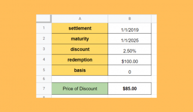
How To Use PRICEDISC Function in Google Sheets

• by Deion Menor
• November 20, 2021

How to Use the PRICE Function in Google Sheets

• June 24, 2023

How to Create a Pareto Chart in Google Sheets

• October 19, 2021

How to Randomize a List in Google Sheets (3 Quickest Methods)

Posted on Last updated: November 3, 2023

Google Sheets’s newly launched “Randomize Range” feature lets users randomize a list. You need to go to the main menu and click on “ Data ” followed by “ Randomize range ” to access this feature.

The Sort and Filter tools in Google Sheets are most commonly used to organize datasets in particular order.

However, there are a few scenarios where you may wish to sort the dataset in a completely random order. For example,

• Sorting student names in random order for group studies or games
• Picking up participants randomly for an event
• Selecting a winner for a giveaway

If you are searching for the quickest method to randomize a list in Google Sheets, then you have come to the right place.

In this article, we will discuss several methods to randomize a list in Google Sheets. It includes using built-in features and functions that may help you now as well as in the future, so make sure to read the article till the end.

Here are the three methods to randomize a list in Google Sheets. You can click on the links to jump to that particular section of the article.

• Using the Randomize range feature – (Quickest Method)
• Using the RAND function and Sort tool
• Using the ARRAYFORMULA function

Copy the Example Google Sheet

Now, before we dive deep into each method of randomizing a list in Google Sheets, consider getting the following Google Sheets data and following me as I take you through this article.

Click Here to!

The example Google Sheet contains datasets used to demonstrate various features and functions to randomize a list.

If you have your own Google Sheet ready to practice the things we are about to discuss, then skip downloading the above file.

Let’s get started now without any further ado!

How to Randomize a List in Google Sheets

As mentioned above, you can choose from various methods to randomize a list.

We will start with the quickest method to randomize a list, then dive deep into using the built-in functions to get almost similar results.

The good thing is you don’t need to be an expert to use any of these methods.

Here is the list of the Giveaway participants,

Task: Our job is to randomize the above list and pick up three winners.

Now, let’s get started.

METHOD #1 – Using the Randomize range feature in Google Sheets to randomize a list

Google Sheets has recently announced this feature to let users quickly randomize datasets.

It is pretty straightforward. Before this announcement, users had to go through a comparatively lengthy workaround to randomize datasets.

Here are the steps,

• Open the Google Sheet
• Select the range you wish to randomize (Note that you need to avoid including the column header while selecting the range. In case you don’t have a header, then simply select the entire column and follow the steps below)
• Right-click to see more options
• Next, choose the “ View more cell actions ” option from the popup
• Click on “ Randomize range “

You will see that all the cells are shuffled randomly, as shown in the above GIF.

If you are not happy with the results, then make sure to use the “Randomize range” feature several times.

Q. What is another way to access the Randomize range feature in Google Sheets?

You have two options to apply the Randomize range to a list.

The first one is to right-click and select the “View more cell actions” option from the popup, as discussed above.

For the second one, here are the steps:

• Go to the main menu
• Click on the “ Data ” tab

Both of them require you to do a few clicks. So, you can choose it as per your preference.

METHOD #2 – Using the RAND function and Sort tool in Google Sheets to randomize a list

This was the most popular method to randomize a list in the past. Before Google Sheets introduced the Randomize range feature, it was my go-to method.

In this method, you need to create a helper column and use the RAND function in Google Sheets to generate random numbers.

Those random numbers are then sorted in ascending or descending order using the Sort tool.

Before we dive deep into this method to randomize a list, let us have a quick look at the RAND function.

Explained: The RAND Function in Google Sheets

The RAND function generates a random number between 0 and 1 without any argument.

Here’s the general syntax for the RAND function,

This function automatically generates a new number each time you open the Google Sheet or perform any calculations within the spreadsheet. In other words, the calculations are real-time and vary depending upon the changes made to the Google Sheet.

Avoid inserting any values or providing the cell references for this formula, as it doesn’t accept them and returns an error.

That’s all about the RAND function. 

Now, let us use it to randomize a list in Google Sheets.

Step 1: Prepare a helper column using the RAND function

We will start by adding a column next to the main list, as shown below.

You can name the column as per your preference. For the sake of simplicity, we have named it Helper.

Now, we will generate random numbers using the RAND function. Here are the steps:

• Click on the cell “ B2 “
• Type “ =rand ”
• Select the first option from the popup or press the “Tab” key
• Close the bracket using “ ) “
• Press “ Enter “

• You will see a “ + “ icon
• Click on it and drag that “+” icon to the end of the table, as shown in the following GIF

Here’s how our helper column looks like,

Note that all the random numbers generated above would change each time you perform a certain calculation on them or even add new entries to the spreadsheet.

For example, I have added random input “ asd ” into the cell “ D1 “. As soon as I do it, the numbers are generated again. Refer to the following GIF.

Step 2: Randomize the dataset using the Sort tool

In this step, we will sort the entire dataset by the numbers generated using the RAND function.

Let’s begin,

• Select the entire table

• Click on the Filter icon

• Go to the cell “ B1 ” and click on the filter icon
• Select the first option, “ Sort A to Z “

Google Sheets will instantly sort the table based on current numbers generated using the RAND function. Also, at the same time, new numbers are generated, which can be used to randomize the list further.

The RAND is a volatile function that allows you to repeat the above process an infinite number of times to randomize a list.

METHOD #3 – Using the ARRAYFORMULA function in Google Sheets to randomize a list

In this method, along with the ARRAYFORMULA, we need to use various built-in functions in Google Sheets.

We will combine all those functions to build a formula as follows,

It is a quite lengthy formula that randomizes a list every time you open the Google Sheets or perform any calculation within the spreadsheet.

Before we dive deep into the actual steps, let us quickly discuss each function used in the above formula so that you will understand how it is built.

Explained: The ARRAYFORMULA Function in Google Sheets

As from the name itself, it is an array formula that has the following general syntax.

The “ arrray_formula ” argument accepts cell range or an expression including the cell range as an input.

So, based on that particular cell range or array size, the function performs calculations. If you don’t put any expression (that includes the cell range), the function will simply display the entire cell range as is.

Explained: The SORT Function in Google Sheets

The SORT is a powerful function in Google Sheets . It allows users to sort datasets by single or multiple columns in ascending or descending order.

The general syntax for the SORT function is as follows,

Here’s how to deal with each argument of the SORT function:

• “ range ” – It needs to be replaced with the cell or table range, which needs to be sorted.
• “ sort_column ” – Here, particularly in the case of the table, you need to define the column which you wish to sort.
• “ is_ascending ” – This argument lets you decide if the sorting should be applied in ascending or descending order. It is an optional argument that accepts “TRUE” or “FALSE” as input.

Note that with the SORT function, you can sort the table using multiple columns.

Explained: The RANDBETWEEN Function in Google Sheets

This function is similar to the RAND function discussed in the second method of randomizing a list in this article.

The only difference is that the RANDBETWEEN function lets you generate random integer numbers within a specified range.

The general syntax for the RANDBETWEEN function is as follows,

The arguments are self-explanatory from the name itself.

• “ low ” – Here, you need to define the lower bound of the range
• “ high ” – It is the upper bound of the range

The function is pretty straightforward. Note that it is a volatile function that updates the random number each time you open the Google Sheet or perform any calculation within the spreadsheet.

Explained: The SIGN Function in Google Sheets

The SIGN function in Google Sheets is used to return the sign of a given number.

It evaluates the sign and returns “1” if it is positive or “-1” if it is negative. Whereas, for the zero as an input, the function returns “0”.

Here is the general syntax for the SIGN function in Google Sheets,

Where the “ value ” argument needs to be replaced with the integer number whose sign needs to be evaluated. You can either manually enter the number or provide the cell reference holding the number.

It is combined with the other functions in Google Sheets to create powerful formulas.

Explained: The ROW Function in Google Sheets

The ROW is a simple lookup function in Google Sheets. It returns the location of a given cell or range of cells.

Simply put, the function returns the row number within a specific cell range.

The general syntax for the ROW function is as follows,

Here, the “ cell_reference ” argument is optional. If you don’t specify any value, then the function will return the row number where you have entered the formula.

You can provide a cell reference or range to this function.

Now that we have learned all the functions let’s combine them to create a formula capable of randomizing a list in Google Sheets.

• Type “ =sort ”
• Select the first option from the popup or press “Tab” key
• Provide the cell reference “ A2:A21 ” for the “range” argument of the SORT function
• Press “ , ” to move to the next argument

• Select the first option from the popup
• Now, for the “array_formula” argument of the ARRAYFORMULA function, we will type “ randbetween “ (Here, we are creating an expression using the RANDBETWEEN function. It will generate a random number for the cell range defined in the ARRAYFORMULA function)

• Type “ sign ”

• Type “ row ”

• Provide the cell reference as “ A2:A21 ” for the “cell_reference” argument of the ROW function
• Close the bracket for the ROW function using “ ) “
• Close the bracket for the SIGN function using “ ) “
• Now, you will be asked to provide the information for the second argument (“high”) of the RANDBETWEEN function. Let’s type “1000” (Make sure to choose the number that will be greater than the size of the column range)
• Close the bracket for the RANDBETWEEN function using “ ) “
• Close the bracket for the ARRAYFORMULA function using “ ) “
• Next, you will be asked to replace the “is_ascending” argument with the proper information. Let us type “ TRUE ” and sort the cell range in ascending order
• Close the bracket for the SORT function using “ ) “
• Press the “ Enter ” key

Here’s how our formula looks after following the above steps,

As you can see from the above GIF, after typing the formula, Google Sheets will instantly sort the names of the participants in a random order.

Note that this is a volatile formula due to the use of the RANDBETWEEN function. It means that if you perform any calculation, add entries, or perform any operation, the sorting will be automatically adjusted.

For example, let us add “ asd ” in the “ D1 “.

As seen in the above GIF, the sorting is automatically updated.

The above methods use built-in functions and features by Google Sheets to randomize a list. Additionally, there are a few third-party add-ons that get the job done for you.

However, with the newly launched Randomize range feature, you don’t need anything else to randomize a list in Google Sheets.

I hope this article was helpful to you.

Feel free to comment below if you are still having any issues or are stuck somewhere while randomizing a list using one of the methods discussed in this article.

Looking forward to answering all your questions.

How to Select a Random Sample in Google Sheets

Often you may want to select a random sample from a dataset in Google Sheets. Fortunately this is easy to do using the RAND() function, which generates a random number between 0 and 1.

The following step-by-step example shows how to use this function to select a random sample in Google Sheets.

Step 1: Create a Dataset

First, we’ll enter the values of a dataset into a single column:

Step 2: Create a List of Random Values

Next, type  =RAND() into cell B2. This creates a random value between 0 and 1.

Copy and paste this formula into every remaining cell in column B:

Step 3: Copy & Paste the Random Values

Next, highlight the values in column B and click Ctrl + C . This will copy all of the values. Next, right click on cell C2 and choose  Paste special > Paste values only .

Note that the values in column B may change once you do this, but don’t worry about this.

Lastly, highlight the values in column C and drag them to replace the values in column B.

Step 4: Sort by the Random Values

Next, highlight cells A2:B16. Then click the Data tab along the top ribbon, then click  Sort range .

Choose to sort by the values of Column B from A to Z, then click Sort :

The values will be sorted based on the random number, from smallest to largest:

Step 5: Select the Random Sample

Lastly, choose the first  n  rows to be in your random sample. For example, if you want a random sample of size 5, then choose the first 5 raw data values to be included in your sample.

In this example, our random sample would include the first 5 values: 5 , 20 , 14 , 13 , 8 .

Additional Resources

The following tutorials explain how to select a random sample from a dataset using other statistical software:

How to Select a Random Sample in Excel How to Select a Random Sample in R How to Select a Random Sample in Python

MSE vs. RMSE: Which Metric Should You Use?

How to calculate compound interest in google sheets (3 examples), related posts, how to create a stem-and-leaf plot in spss, how to create a correlation matrix in spss, excel: how to use if function with text..., excel: how to use greater than or equal..., excel: how to use if function with multiple..., how to convert date of birth to age..., excel: how to highlight entire row based on..., how to add target line to graph in..., excel: how to use if function with negative..., how to extract number from string in pandas.

How To Randomize A List In Google Sheets

Last Updated on January 2, 2024 by Jake Sheridan

Generally when people think about the order of data in a spreadsheet, they want to sort that data in a specific way.

But you may also run into situations where you need to randomize a list in.

For example, if you want to create random break out or study groups for a meeting or class.

Instead of trying to randomize a list manually or relying on complex formulas to randomly select each entry from the sorted list, you can automatically randomize a range in Google Sheets quickly in just a few clicks.

Step 1) Access the randomization feature

Step 2) confirm the randomization, step 3) repeat if necessary.

Here’s how shuffle rows in Google Sheets:

Select the range you want to randomize, excluding headers.

Randomization is done based on rows, so you must select at least two rows, however you can select any number of columns

Open the Data menu and click on the Randomize Range option

The rows in the selected range will be sorted into a random order. Note that any blank rows in the range will be moved to the end of the list

You can repeat the process as needed to get a different random order of the rows in the selection

Example Spreadsheet: Make a copy of the example spreadsheet

In this tutorial, I covered how to randomize a list in Google Sheets. Want more? Check out all the Google Sheets Tutorials .

More ways to sort in Google Sheets:

• How To Sort
• Format Dates
• Stop Google Sheets From Changing Dates
• Sort Alphabetically
• Arrange Numbers In Ascending Order
• Sort By Color
• Sort By Date
• Change Date Format
• Sort By Number
• Sort By Last Name
• Sort And Filter
• Sort Unique Values
• Sort In Google Sheets And Keep Rows Together
• SORTN Function

You might also like:

How to Randomly Pick a Name from A Long List in Google Sheets

Do you plan to run a raffle from a long list of names in your spreadsheet? Well, here is a quick solution you can implement in Google Sheets! Here are the steps:

Step 1 : Open the workbook containing the long list of names to pick from. We will use this list of 41 fruits for this tutorial.

Step 2 : On the cell where you want to write down the selected entry, add this formula:

=index(<range_of_list>,RANDBETWEEN(1, <number_of_entries>))</number_of_entries></range_of_list>

Where <range_of_list> is the range of the cells containing the list and the <number_of_entries> is the number of entries contained in the list. </number_of_entries></range_of_list>

The RANDBETWEEN function randomly selects an integer from 1 to a specified maximum number. The maximum number should match the number of items in the list.

If you are not sure of how many entries are in the list but they are all in a single column , you can write the range as follows:

<first_cell_in_the_list>:<column_letter_of_the_list></column_letter_of_the_list></first_cell_in_the_list>

So for our example, we can write our range as A1:A, setting the first entry as A1 and then followed by all the cells with entries in column A. To replace <number_of_entries>, we can use the COUNTA function, defining its range in the same manner:</number_of_entries>

COUNTA(<first_cell_in_the_list>:<column_letter_of_the_list>)</column_letter_of_the_list></first_cell_in_the_list>

Plugging them together, we can have

=index(<range_of_list>,RANDBETWEEN(1, COUNTA(<range_of_list>)))</range_of_list></range_of_list>

This equation is more flexible because it allows you to add or remove entries in the list!

Once you entered the formula, Google Sheets will then select an item from the list

The RANDBETWEEN function runs whenever there is a change in the spreadsheet. You can type a random character on a blank cell and it will change the selected entry. Pretty neat, right?

• 27 pages of Google Sheets tips and tricks to save time
• Covers pivot tables and other advanced topics

Work less, automate more!

Related articles.

Automatically Create PDFs from Google Sheets (2024 Update)

How to generate google sheets invoices (easiest way 2024), create a google calendar event from google sheets.

The Ultimate Guide to Google Sheets Automation (2024)

A Guide to Auto-Assignments in Google Sheets

In this guide, we'll look into using the `onFormSubmit(e)` installable trigger which will let us apply automation to any new tasks being created through the Google Form we created in the guide to basic task management

Similar to our guide on checkbox automation , this guide will also require some knowledge of javascript.

There are several ways to approach auto-assignments. At the end of the day, the point is just to make sure that someone on your team is assigned to any new tasks coming, even if they might re-assign it to someone else. In this guide, we'll go over three types of auto-assigning logic:

• Round Robin

Dynamic Equal Distribution

But first, let's make sure our spreadsheet is set up properly.

Create a Named Range for your Assignees

Doing this is pretty simple. In your "Settings" tab, create a list of Assignees if you haven't already. Then highlight the entire column, click on the "Data" option in the menu bar, and select Named Ranges. Let's give it the name "Assignees".

Not sure how to make a named range? Check out our how-to on named ranges for detailed instructions

Set up the trigger

Before diving into the code, let's set up the `onFormSubmit` trigger you'll be using. It'll be handy to have when you start writing the code and need to test it. To set up this trigger, you'll have to create something called an "installable trigger". It's easy to do this though - click on the "Triggers" option in your Script Editor and then find the "Add Trigger" button on the bottom right.

On the options, make sure to set the "event source" as "From spreadsheet" and the "event type" as "On form submit". For the "which function to run" option, you'll have to come back to this later on to set that.

Create the Logic

At a high-level, the logic is pretty straight forward. If we were to explain it in words, it would be:

- Get a list of the assignees available

- Figure out who the next assignee is

- Find the newly created task

- Set the "Assignee" field to the next assignee

Each approach will have their little nuances, but they'll all follow these basic steps.

Shared Logic

For the list of assignees, we're going to retrieve the named range we created by calling the `SpreadsheetApp` library in our script editor and using some pre-built functions to find the named range. It'll look like this:

Once we have this range, we'll need to filter it down so that we just have the names of our assignees in it. This means we'll need to remove the header row and also any blanks that exist. We'll dot his using javascript's `.filter()` function.

Keep this somewhere safe for now. We'll be using it in the next three parts.

Value Setting

The other bit of logic that will be shard across all methods is how we set the "Assignee" field to the qualifying assignee. To do this we'll have to find the cell we want to update and then set it to the output of our assignment logic. Just like the `OnEdit(e)` function, we'll be utilizing the `e` parameter which is just short for event. We just need the row for this logic, so we'll be doing something like this:

We're also going to make use of the `getColumnByName()` we wrote in the previous guide . Here's what the line of code will look like:

We'll be using this in the next 3 parts, so put this in a safe place like you did with the logic for assignees.

Random Assignment

The differentiating part for randomly assigning tasks to team members is being able to randomly pick someone from the list of team members. To do this, we'll need the list of assignees (using the code above) and also a way to generate a random number. Luckily, javascript gives us a way to do this by using `Math.random()` which will give us a random value between 0 and 1. We're going to use that in combination with `Math.floor()` which will give us the largest integer based on what we give it. For example, if we did `Math.floor(5.5)`, it would give us 5.

Since `Math.random()` only gives us values between 0 and 1, we'll also need to multiply it by something so that we get something larger than 0. Since we need the number generated to match up with the number of assignees we have available, we'll just use the count of assignees. Here's how our line of code will look:

The output of this should be an integer between 0 and the number of assignees you have. To figure out the assignee's name, all you need to do is set our `assignment` variable to `assignee[rand]` which will give you the assignee in the Nth index position of your assignees array.

When you combine this logic with the assignees and the value setting logic, your entire `assignByRandom()` function should look like this:

To test this, go back to the triggers page and update the trigger we created to use the `assignByRandom()` function.

Round Robin Assignment

The round robin logic is going to be a lot more involved than the random logic. For the round robin, we'll have to keep track of who the last team member was that got assigned to a task. In order to do that, we'll be using a built-in feature of Google Apps Script called "Properties Service". In a nutshell, this service let's us store information in the script without having to save it in a database - it's perfect for remembering who the last assignee was.

To call the "Properties Service" we'll do something similar to how we call the `SpreadsheetApp`. For this, the command will be `PropertiesService` and we'll call the `getScriptProperties()` function. Let's set that to the variable `script_properties` and then try to retrieve a property called "previous":

Notice that we used `parseInt()` when grabbing the "previous" property. This is just a way to make sure that what we're getting back is in integer since we'll need it to get the index position of our assignee array. Please note, if there is no property for "previous" that it'll just get returned to us as "undefined". We'll have to take that into account in our next block of code.

A lot to unpack here. Let's start with the `if` statement. In our criteria, we're checking to see if the "previous" property is undefined and also to see if the "previous" property is equal to the number of assignees on our list. We're subtracting one from the count of assignees because arrays start from 0.

If our criteria is met in the `if` statement, we're setting the "previous" property to 0 since we're either running this logic for the very first time, or we have to reset the counter because we've reached the end of the assignee list. We're using `script_properties.setProperties()` to update the "previous" property.

When the "previous" property is not undefined and it is less than the number of assignees we have, we want to iterate it by one and set that as the new value. This will make it so that our next run gives us the index value of the assignee we're about to assignee to the new task during this run of the logic.

The next part is similar to what we did in the random logic - we're going to set the `assignments` variable to `assignee[next_assignee]` which will give us the person that's next in line to get assigned. once you combine this logic with the assignees and the value setting, it'll look like this:

That's it for the round robin logic. If you have 3 team members, it'll go in order of the list -- 1, 2, 3, 1, 2, 3 and so on. This is a very popular way of auto-assigning tasks. The only problem with it is that it doesn't care if someone is overburdened with tasks or not.

To test this, go back to the triggers page and update the trigger we created to use the `assignByRoundRobin()` function.

This method will take a look at the distribution of tasks and then assign the new task to whomever has the least amount of tasks. I personally like this method because it ensures that everyone is getting equal treatment at all times even if the team re-assigned tickets around and ended up giving someone more than the others. It's a great way to make sure that everyone on the team pulls their weight.

In order to figure out the distribution of tasks, we'll need to get the full list of tasks we have. We'll be using the `getRange()` function, the `getColumnByName()` function, the `getLastRow()` function, and also the `flat()` function. Our line of code will look like this:

Notice how we're using 4 paramters in the `getRange()` function instead of the usual 2 that we did in the checkbox automation guide. The other two parameters is the `number_of_rows` and the `number_of_columns`. This lets us get a range of data instead of a single cell. The `getLastRow()` function will give us very last row index available on the sheet that has data. We only care about the "Assignees" column, so the number of columns is set to 1.

The `flat()` function we're using is just to make it so that our array of assignments doesn't have any nested arrays in it. It'll make it easier for us to filter things out in the next block of code:

In this code block, we're doing a couple of things that are important. The first thing is declaring a brand new array that we're going to use to store the count of tasks for each assignee. The second thing we're doing is looping through each assignee and filtering down the list of tasks for items that are assigned to them. We're using javascript's `filter()` function to do this, similar to how we cleaned up the assigneees list earlier.

Now that we have a set of assignment counts for each assignee, the next step here is to figure out which one has the lowest count. To do that, we're going to set a variable to the lowest amount and compare each index in the array to the amount - if the value in the array is lower than the amount, then we'll use that as the new benchmark and save the index. We'll keep doing this until we've gone through the entire list and the end result should tell us what the lowest amount was and which index position it was in within the array.

Since we filled in the `assignees_count` array in the same order as the `assignees` array, the index position of the arrays will match up. Because they match up, we can use the index position of the `assignees_count`'s lowest value to find the matching assignee's name on the `assignees` array. Allowing us to do this:

Looks familiar right? the next and final step here is to combine it with the assignees logic and the value setting logic - giving us this function:

To test this, go back to the triggers page and update the trigger we created to use the `assignByEqualDistribution()` function. If everything was set up right, every new form submission made through the Google Form willget assigned to whomever has the least number of tasks.

Clean up Your Code

It's always good to clean up your code so that they're not repeating code in different places and also so that you can read it better. In our cleanup, we're going to explore using multiple files in the Script Editor and refactoring our code so that we're following a DRY method (aka "don't repeat yourself")

Using Multiple Files in Google Apps Script

The first step of cleaning up your Google Apps Script project is to separate your functions out from a single file and into multiple files that are grouped by type. You can create new files by clicking on the "+" icon and selecting the "Script" option. The "HTML" option is for UI options, which we'll cover in another guide.

If you need to rename a file, just hover over the file name, click on the 3 dots, and then select the "rename" option:

Based on everything we've done in this guide, you'll want about 4 files of separation to have it nice and neat.

### DRY'ing Our Code

There are two code blocks that we consistently used in this guide. The first one is for retrieving the assignees list and cleaning it up. The second is finding the row we want to update and setting the new assignee value to it. To clean this up, we'll want to extract that code from the 3 different assignment functions and make it more generalized.

If we create a new function to handle this, it'll look like this:

This function will handle retrieving the list and then cleaning it up. This will let us set up the beginning of the other 3 functions like this:

By doing this, any changes we make to the `getAssignees()` function will be shared across all 3 functions.

Next up is the value setting logic.

Just like the `getAssignees()` function, this change will let us update all 3 functions by updating the logic in one spot.

If you're feeling confident, there's another thing we haven't done, which is auto-setting the status. You can do this by adding in another line of code to each of the 3 assignment functions which would update the Status field. Hint: it should happen around the same time as when you're updating the Assignee field.

This is the end of our series on creating a basic task management tool in Google Sheets. If you've gotten this far, your task management tool should have:

• An entry form
• A basic reporting dashboard
• Dropdown selections
• Conditional alerts
• Dynamic Todo lists
• Dynamic backlinks to tasks
• Automated status updates on the Todo lists
• Auto-assignments for new Tasks

You might also like...

COMPLETE Guide to Event Triggers w/ 5 examples

In this video, we'll go over 5 examples of using Event Triggers to help you go from doing tedious work to being a SUPERCHARGED automation…

Easiest Way To Upload Responses to Google Forms

We all wish that uploading responses to your Google Form was as easy as inserting new rows into the linked Google Sheet, but it's not... It…

Adding a Custom Sidebar w/ Tabs to Google Sheets

Adding custom sidebars into your Google Sheet gives you so much more flexibility with the user experience - but it only gives you 300px of…

Randomly Assign Teams in Google Sheets

• May 4, 2023
• Google Sheets Tutorials
• Ryan Morton

In this article, you will learn how to set up Google Sheets to randomly assign a group of participants to any number of teams.

Once you set up the spreadsheet, you only have to click twice to assign everyone to a team. And if you don’t like the results, you can re-randomize the assignments again!

Before getting into any functions or formulas, you need to set up your spreadsheet. Start by listing the team names across columns in row 1.

Next, list the participants in a single column to the right of your team names.

With your spreadsheet setup like this, you are ready to compose the formula .

The Formula

Add the following formula to cell A2.

This formula uses the WRAPROWS function to take the participants and split them up across all of the teams.

The first argument of the WRAPROWS functions references the range of cells containing all of the participants. In this case, the participants are listed in the range of E2:E10.

The second argument of the WRAPROWS function is the number of teams you have. In this example, there are three teams.

With your formula set up, all that’s left is to randomize the assignments.

Randomize the Range

To randomize the team assignments, you must randomize the original participant list.

To do this, select the range of cells containing the participants. With this range selected,  right-click  and select  View more cell actions , and then  Randomize range .

This will shuffle the list of participants, thereby resulting in randomized team assignments.

And that is how you can randomly assign teams in Google Sheets.

See It In Action

Check out the video below to see this method demonstrated in Google Sheets.

This Post Has 0 Comments

Leave a reply cancel reply.

Your email address will not be published. Required fields are marked *

Save my name, email, and website in this browser for the next time I comment.

Notify me of new posts by email.

This site uses Akismet to reduce spam. Learn how your comment data is processed .

Related Posts

How Location Affects Formula Syntax in Google Sheets

Lookup the Smallest or Largest Value

How to List Missing Values in Google Sheets

• previous post: Build a Heat Map in Google Sheets
• next post: Filter by Color in Google Sheets

Privacy Overview

Generate random numbers, dates, passwords

Random Generator will help you get the type of random data you need in your Google sheet. Fill cells with numbers, Booleans, dates, passwords, etc. in three simple steps: select the cells, choose the type of data, and click Generate . Please see the detailed instructions below.

Before you start

How to use random generator, start the add-on.

How to generate random integer numbers

• Use the From and To fields to change the default range of integer numbers to be picked. You can enter any negative or positive number. Note. The From and To fields cannot be empty. If you delete a value, the default one or the one you entered previously will appear in the field.
• Have only unique integers generated by ticking off the Unique values checkbox. Otherwise, the range will be filled with random integers that can be repeated.
• Click on the Generate button and get random values in your selected range.

How to generate random real numbers

• Use the From and To fields to change the default range of real numbers to be picked. You can enter any negative or positive number. Note. The From and To fields cannot be empty. Delete a value, and the default one or the one you previously entered will appear in the field.
• To generate only unique real numbers, check the Unique values option. Or leave it unchecked to fill the range with random real numbers that can be repeated.
• Click Generate and see the range filled with real numbers randomly.

How to generate booleans at random

• The Value drop-down list has the TRUE/FALSE option selected by default. Change the value to YES/NO if necessary. Tip. The add-on will remember the latest chosen option.
• Click  Generate  to fill the selected cells with these values at random.

How to generate random dates

• Change the dates by picking a day in the calendar that pops up when you click on the From and To fields. Tip. The add-on will remember the latest entered dates.
• Choose to generate only Weekend or Workday dates by selecting the corresponding checkboxes. Tip. Tick off both options and the add-on will populate your range with both weekend and workday dates.
• Select the Unique values checkbox and have only unique dates generated. Otherwise, the range will be filled with random dates that can be repeated.
• Click Generate and get random dates within your selection.

How to generate values from custom lists

Or you can create and use your own lists instead:

• Create and select the range of values you want to add as your custom list.
• Click on the New list button.

• Click OK to save the list.
• If you want to have random custom list records without duplicates, tick the  Unique values  checkbox and all the generated entries will differ.
• Press Generate to populate the cells with the items from your list randomly.

How to generate random strings

• Select the checkboxes next to the necessary character sets, the add-on will remember your choice: A-Z , a-z , 0-9 , punctuation marks , space , and hexadecimal .
• If you choose Custom character set, enter the chars you need there. Otherwise, default characters will appear in this field.
• To generate strings by length, select the String length radio button and enter the number of characters you want in a line.
• To generate random values By mask , either select from default patterns in the drop-down list, for example, (????)-????-????? , or enter your own mask using the question mark for one random character and any repeating symbols. Note. Make sure to enter at least one character in this field.
• Click Generate to fill the selected range with passwords or strings according to your settings.

Related pages

• Shuffle data in Google Sheets
• Change multiple formulas in Google Sheets

Good day. I would like to find out if duplicate numbers can occur when generating unique numbers on different days. In other words, can a duplicate number ever be generated from a person's account?

Hello Lara,

Thank you for your comment.

Please check the Unique values option if you want just unique numbers to be generated. Also, if you need to check your list for duplicates, you can use our Remove Duplicates tool.

If you have any other questions or need further assistance, please feel free to email us at [email protected] .

Hi, I'm wondering if the key license work on multiple devices and multiple Google account? I'm purchasing for company. Thank you.

Thank you for your question.

Please note that a subscription for the Google Sheets add-on is account-based. If the product is going to be used under different Google accounts at the same time, you need to have several subscriptions, so there is one for each account. However, we don't impose any limitations on the number of devices or people who can work with the add-on at the same time, as many of your colleagues as you need can use the add-on under the same account on different PCs.

Please email us at [email protected] with the subscription plan you'd like to get and the number of users who need access to the add-on. We'll provide you with the pricing details and a direct link to the purchase order form. Thank you.

Dear Support Team, I would like to use this Plugin to generate random but unique identifiers to my customers. However with random strings I cannot set that the new values should be unique. Do you have any solution how to avoid duplicates? Thank you for the answer.

Each group of values (except Boolean and String) offers this option – Unique values . All you need to do is tick it off and no duplicates will be generated. The String group generates unique records by default. I kindly ask you to look through the instructions closely, you will find the text description of the option and will see it on the screenshots.

I purchased this by mistake! Is there any way I can cancel and get a refund for my subscription?

Hello, Moriah,

Thank you for contacting us. I'm sorry you've encountered this problem.

Please email us to [email protected] with your order ID and the email address you purchased the subscription for.

We'll do our best to assist you. Thank you.

Post a comment

Seen by everyone, do not publish license keys and sensitive personal info!

How-To Geek

How to generate random numbers in google sheets.

Quickly generate random numbers in your spreadsheets with this Google Sheets function.

Google Sheets provides a simple function to generate random numbers inside your spreadsheet without having to leave the document or install an add-on . The function returns a random integer between two values. Here's how to use it.

Fire up the  Google Sheets homepage and open either a new or existing spreadsheet. For this guide, we'll use the function RANDBETWEEN to produce a random number .

By default, the RAND function only generates a number between 0 (inclusive) and 1 (exclusive), whereas  RANDBETWEEN lets you specify a range of numbers. While you could modify the function to generate other ranges, the RANDBETWEEN function is a much simpler way to accomplish this.

Related: How Computers Generate Random Numbers

Click on a cell where you want to insert a random number and type

but replace

 with the range in which you want the random number to fall.

For example, if you want a random number between 1 and 10, it should look like this:

=RANDBETWEEN(1,10)

After you fill in the range, press the Enter key. The random number will populate the cell where you entered the formula.

If you want to use a number from another cell in your spreadsheet, all you have to do is enter the cell number instead of a low or high number.

Note:  Both RAND and RANDBETWEEN are considered volatile functions, meaning they don't retain the data in the cell forever. So, when you're using either of the functions, they recalculate a new number each time the sheet changes.

If you want to change the interval in which your random number is recalculated, open up File > Spreadsheet Settings, click on the "Calculation" tab, and then choose how often you want the function to recalculate from the drop-down menu.

You can select "On Change" (default), "On Change and Every Minute," or "On Change and Every Hour." Click "Save Settings" to return to your spreadsheet.

How to Assign a Task in Google Sheets [Easy Guide]

• Last updated January 17, 2024

To assign a task in Google Sheets, either tag someone’s email in a comment or create a drop-down list. I show both methods in this guide.

The commenting method is used in Google Docs, Google Sheets, and elsewhere in the GSuite. The drop-down method of assigning tasks is unique to Google Sheets.

Table of Contents

How to Assign a Task in Google Sheets with a Comment

To assign a task to someone in Sheets, you must set it using a comment. In Google Sheets, you can assign tasks by commenting on the message in the comment box and adding the person’s email. You will then be prompted with an option to assign tasks in Google Sheets.

Here is how to assign in Google Sheets:

• Open the spreadsheet where you want to assign the task.
• Click on the cell or select multiple cells by clicking and dragging your cursor across several cells. You can also select a single cell and then drag your cursor on the blue dot in the bottom right corner of the cell.

• Click on Insert or right-click on the selected area. This selected area is represented with a light blue highlight. This will open a dropdown menu.
• There, click on Comment . You can use the Ctrl+ Alt+ M  shortcut on Windows to do this.
• In the comment box that shows up, type in the comment and add the At  ( @ ) sign.
• Now add the email of the person.
• A new Assign  option will show under the email when you add the email Click on the Assign to [email]  button.

• Click on the green Assign  button.

The assignee will receive a notification and can mark the task as done when they finish it. There is a difference between adding normal comments and assigning a task. When a normal comment is made, anyone can make the changes and mark it as done. However, using the assign task Google Sheets function means that only the person assigned the task can mark it as done.

How to Use a Drop-Down List to Assign Tasks

While the comment method gives helpful email reminders, sometimes it’s helpful to have a dropdown menu that shows who’s working on what. Here’s what you’ll need to know to create a drop-down menu to assign tasks in Google Sheets.

Here’s a visual walkthrough. First, you’ll select the cell where you want the dropdown menu. Then, click the “insert” menu and choose “dropdown”.

Then, you’ll see an option to choose “criteria”. Choose “dropdown from a range” if you already have an existing list with the name of the user or users you want to use.

Next, you’ll select your data range. Here, my range is F2:F5 on my main sheet. If yours is on another sheet, you can go to that tab to make your selection.

Finally, you’ll choose colors for the dropdown. Each person on your team gets a different color. That makes it easy to distinguish who’s working on what task. Here’s what my sheet looks like after I chose the colors for each task owner.

You’ll notice my task-tracking spreadsheet also has checkboxes. I don’t need a bunch of checklist text to see whether a task is completed. My team just clicks the box and I know we’re done with each project.

Video Guide

Here’s my video guide on how to assign tasks in Google Sheets. I covered both methods, commenting and drop-down menus.

What Happens When a Task Is Assigned?

When you assign a task to someone, they will get an email and a notification in Google Sheets .

If you’re not a part of the spreadsheet, you will receive the permissions through a link in your email. If you are already a team member in the spreadsheet, when you open Google Sheets, you will see a grey dot with the number of the assigned tasks inside it.

When completing the tasks, they can click on the checkmark in the comment box to mark it as complete. You can also look at the previous and current tasks by going to the comment history section in Sheets. Just remember to enable edit access if you want them to mark check boxes in your spreadsheet.

How to Maximize the Google Workspace

Here are some of the best ways to get the most out of your spreadsheet task list.

• Task owners should mark their tasks in Google Calendar to get regular reminders prior to the due date.
• Workspace admins should regularly review access to make sure task owners can access what they need.
• Workspace admins should consider automation to reduce repetition.

When in doubt, remember the basics of project management. You may want to consider something like Jira , which is a popular tool for project and issue tracking.

Common Mistakes

Here are some of the most common mistakes I see when assigning tasks in Google Sheets.

• Missing Access

If you tag someone in a comment, they’ll need the ability to see the document to interact with your task. Google’s spreadsheet software is smart enough to remind you of this. But don’t cancel the warning message if you try to tag someone who isn’t already listed as a collaborator in your workbook.

• Missing Notifications

If you’re using a dropdown menu to assign tasks, remember that your assignee won’t get an email notification. Dropdown menus give you a bunch of visibility into who’s working on a task and who’s responsible for it (see my RACI templates ), but they don’t give you the same kind of cloud-based communication you get with a comment.

• Missing Information

When you use the dropdown method instead of Google’s standard comment method of assigning tasks, sometimes it’s hard to tell what happened in the past. If you want to know about the previous assignee or older comments, you’ll want to use the commenting method instead. It’s one of the easier ways of tracking conversations about a specific topic in Google Sheets.

• Missing Automation

Those who use a spreadsheet as task management software will want to automate tasks. For that, you’ll want to familiarize yourself with app script . There are many things you can do when you add more complex scripts into your workbook. For example, you may want to automatically assign items on your task list. Or you may want to automatically populate an assignee’s task list. Scripts make this easy.

Why Assign Tasks in Google Sheets

Running a team in Google Sheets is among the best uses for the program. But, it can be annoying to assign tasks in other programs and then move them into Sheets. Luckily, you can assign tasks directly in Sheets through the comment menu.

Assigning tasks can be a helpful feature in Google Sheets as it allows you to individually assign the things to do rather than just leaving comments. This has one crucial advantage as it tells everyone what to do and only the person assigned a task completes it rather than anyone in the team making the changes.

Doing this has several benefits. You can divide the workload appropriately among your team members, and there won’t be any confusion about what a person needs to do. The tasks as marked for that specific person, so they don’t have to go through a list of comments to find their task.

Assigning specific tasks is more effective project management .

Frequently Asked Questions

If you’re interested in assigning tasks in Google Sheets, you may have follow up questions. I’ll do my best to answer those that come up most frequently, but please feel free to leave a comment below. And remember, I also have a YouTube channel where I offer video guides.

How Do I Assign an Action in Google Sheets?

• Click on the cell or select multiple cells.
• Click on Insert or right-click on the selected area. This selected area is represented with a light blue highlight. There, click on Comment.
• Add the email of the person. A new option will show under the email when the email is added.
• Click on the Assign to [email]  button.
• Click on the green Assign button.

How Do You Assign a Task to a Spreadsheet?

The Google Sheets assign tasks function is accessed through the comments menu. You can assign tasks by commenting on the message in the comment box and adding the person’s email. You will then be prompted with an option to assign tasks in Google Sheets.

Does Google Have a Task Manager?

Google offers a mobile application called Tasks. This allows you to edit, manage, and capture the tasks from anywhere and at any time. This also allows full synchronization among the tasks on multiple devices.

Can I Delegate Google Tasks?

You can add the email of a person that isn’t already added to the spreadsheet. This will send them an email and a link to the file. When they click on it, they will get access to the file and make the changes normally as if they are a part of it. You could also build a schedule  to help with delegating tasks.

Wrapping up How to Assign Tasks in Google Sheets

We hope that learning how to assign a task in Google Sheets through this guide was easy for you. It’s one of those skills that when you’ve done it once you can do it 1000 times. Let us know in the comments if you need any help.

Related Reading:

• How to Make a Google Sheets Button [Easy Guide]
• Step-by-Step Google Sheets Permissions Guide
• 5 Useful Google Sheets Project Management Templates [Free]
• How to Connect Google Forms to Sheets
• Can Google Sheets Track Changes? Yes! Here’s How

Most Popular Posts

How To Highlight Duplicates in Google Sheets

How to Make Multiple Selection in Drop-down Lists in Google Sheets

Google Sheets Currency Conversion: The Easy Method

A 2024 guide to google sheets date picker, related posts.

How to Insert a Google Sheets Hyperlink in 5 Seconds

• Chris Daniel
• April 15, 2024

How to Import Stock Prices into Google Sheets

• April 2, 2024

How to Calculate Age in Google Sheets (2 Easy Methods)

• Sumit Bansal
• February 21, 2024

How to Hide Gridlines in Google Sheets

• February 14, 2024

Thanks for visiting! We’re happy to answer your spreadsheet questions. We specialize in formulas for Google Sheets, our own spreadsheet templates, and time-saving Excel tips.

Note that we’re supported by our audience. When you purchase through links on our site, we may earn commission at no extra cost to you.

Like what we do? Share this article!

How To Generate Random Numbers In Google Sheets

Here are a few useful formulas for generating random numbers in Google Sheets:

Random number between 0 and 1 :

Random whole number between low and high :

Random decimal number between low and high :

Multiple random whole numbers between low and high with no repeats:

Keep reading for more formulas and explanations about how these ones work.

Can you generate random numbers in Google Sheets?

Here's how to:

• Between 0 and 1
• Whole numbers
• Decimal numbers
• Create a button to refresh random numbers
• Stop random numbers from changing

Getting Random Numbers In Google Sheets

Random numbers between 0 and 1.

There's a function in Google Sheets that generates random numbers between 0 (inclusive) and 1 (exclusive):

It doesn't accept arguments like most functions. Instead you simply open and close the brackets and get a random decimal number that's >= 0 and < 1 .

Put another way: 0 <= RAND() < 1 .

Here's what it looks like (click the checkbox to refresh):

Random Numbers Between Any Two Numbers

Get whole numbers.

Once again, Google Sheets has a function for exactly this:

You get a random integer (whole number) between the low and high (both inclusive).

Put simply: low <= RANDBETWEEN( low , high ) <= high

Some common uses of this function is to get a random number from 1 to 10 or 1 to 100 .

Here's an example of getting a random number from 1 to 100 (click the checkbox to refresh):

You can closely replicate the functionality of the RANDBETWEEN function using the RAND function from above:

However, this formula is inclusive of the low and exclusive of the high .

To make it inclusive of both low and high you can use:

Get Decimal Numbers

If you need a decimal number between a low and high you'll need to use a formula.

This is inclusive of the low and exclusive of the high .

Another option is:

However, this function calls for a random number twice which makes it less efficient to calculate.

Here's an example of the first formula generating random decimals between 1 and 100 (click the checkbox to refresh):

Generate Random Numbers With No Repeats

Ensuring there are no repeats in random number sets generated by Google Sheets is difficult because the nature of randomness allows repetition.

The way to get no repeats is a little hacky but it gets the job done.

The trick is that if you want 5 non-repeating random numbers, you need to:

• Generate more than 5 random numbers (using the RANDARRAY function)
• Get the unique numbers (using the UNIQUE function)
• Show only 5 of them (using the ARRAY_CONSTRAIN function)

By generating more than 5 random numbers you increase the likelihood that at least 5 of the numbers will be unique - and that's what you really want. In the examples below you will generate 10 times the required amount of numbers.

There is a small chance that all of the numbers you generate do repeat.

But it's so unlikely that you don't need to worry about it.

If you need random numbers from 0 to 1 , you can use:

Here's what that will look like for 5 random numbers (click the checkbox to refresh):

If you need random whole numbers from low (inclusive) to high (exclusive) :

This is an example with 5 numbers between 1 and 100 (click the checkbox to refresh):

This formula (and the next one) is built based on the structure of the formula to get decimal numbers between any two numbers from above :

This formula is able to accept an array of random numbers (generated by the RANDARRAY function) and output an array because it's wrapped in an ArrayFormula function.

If you need random decimal numbers from low (inclusive) to high (exclusive) :

Here's an example that pulls 5 decimal numbers between 1 and 100 (click the checkbox to refresh):

FREE RESOURCE

Google Sheets Cheat Sheet

12 exclusive tips to make user-friendly sheets from today:

You'll get updates from me with an easy-to-find "unsubscribe" link.

How To Create A Button To Refresh Random Numbers In Google Sheets

To refresh random numbers in Google Sheets you need to change a value.

This is because functions that generate random numbers ( RAND , RANDBETWEEN , and RANDARRAY ) are volatile . This means they update whenever a change occurs in the sheet.

You can make a 'button' to generate random numbers by adding a checkbox somewhere in your Google Sheet.

Simply select a cell and go to Insert ➜ Checkbox in the main menu.

When you click on a checkbox in Google Sheets the underlying value in the cell changes from FALSE to TRUE (and vice versa for unchecking).

This is a change in the spreadsheet and is all that needs to happen for random numbers to refresh.

Here's an interactive example of what that looks like in a Google Sheet:

How To Stop Random Numbers From Changing In Google Sheets

As mentioned above, functions that generate random numbers ( RAND , RANDBETWEEN , and RANDARRAY ) are volatile .

Volatile functions recalculate every time a change (to the contents or structure of a sheet) is made in a Google Sheet.

Examples of 'a change' include:

• Contents: data being added/removed/amended, or
• Structure: columns/rows being added/removed

Formatting changes (like text or cell color) do not trigger recalculation of volatile functions.

The volatility of these functions can cause changes that you don't want (which is really annoying):

And/or slow down your sheet considerably:

If these things are happening to you, you'll want to freeze the random numbers to keep them from changing in your Google Sheet.

To make this happen you need to remove the formulas. Here's how:

STEP 1: Select the cells you want to stop from changing.

STEP 2: Copy the selection you've made. You can use Ctrl+C (Windows) or ⌘+C (Mac).

STEP 3: Paste the selection as values where it is now. You can use Ctrl+Shift+V (Windows) or ⌘+Shift+V (Mac).

Now you have the required data without the formulas.

No formulas means no volatile functions and nothing to recalculate.

You might like:

How To Subtract In Google Sheets

Google Sheets is good at subtracting... you can be too. Learn how to subtract numbers, columns, dates, times, percentages, all of it!

COUNT Google Sheets Function [With Quiz]

The COUNT function in Google Sheets tells you how many numbers are present in a dataset, ignoring everything else. Learn how to count here.

How To Round In Google Sheets

Need to round up and down in Google Sheets? Find out how to round using both formulas and formatting on both desktop and mobile.

Want Better-Looking Google Sheets?

Get my 12-tip cheat sheet that will make your spreadsheets more user-friendly.

• Get One: Tornado Alert Apps
• The Best Tech Gifts Under $100

Generate Random Numbers Using Google Sheets RAND Function

Get a random number between 0 and 1

In This Article

Jump to a Section

• How the RAND Function Operates
• The RAND Function Syntax and Layout
• About the RAND Function and Volatility
• Generate New Random Numbers With Refresh
• Step-by-Step: Change RAND's Refresh Frequency
• Step-by-Step: Enter the RAND Function
• Generate Random Numbers Between 1 and 10 or 1 and 100
• Generate Random Integers Between 1 and 10

One way to generate random numbers in Google Sheets is with the RAND function. By itself, the function creates a limited range when it comes to generating random numbers. Using RAND in formulas and by combining it with other functions, the range of values can easily be expanded.

How the RAND Function Works

By specifying the high and low values of a  range , RAND can return random numbers within a specified range, such as 1 and 10 or 1 and 100.

The function's output can also be reduced to integers by combining the function with the TRUNC function , which truncates or removes all decimal places from a number.

In Google Sheets, when generating a random value between 0 and 1, the RAND function returns a random number between 0 inclusive and 1 exclusive. While it is usual to describe the range of values generated by the function as being from 0 to 1, in truth, it is more exact to say the range is between 0 and 0.99999999...

The formula that returns a random number between 1 and 10 returns a value between 0 and 9.99999...

The RAND Function Syntax

A function's syntax refers to the layout of the function and includes the function's name, brackets, comma separators, and arguments .

The syntax for the RAND function is:

= RAND ( )

Unlike the RANDBETWEEN function, which requires high- and low-end arguments to be specified, the RAND function accepts no arguments.

The RAND Function and Volatility

 The RAND function is a  volatile function  that, by default, changes or recalculates every time the worksheet changes, and these changes include actions such as the addition of new data.

Furthermore, any  formula  that depends either directly or indirectly on a cell containing a volatile function also recalculates every time a change in the worksheet occurs.

Therefore, in  worksheets  that contain large amounts of data, volatile functions should be used with caution, as they can slow down the program's response time due to the frequency of recalculations.

Generating New Random Numbers With Refresh

Because Google Sheets is an online spreadsheet program, the RAND function can be forced to generate new random numbers by refreshing the screen using the web browser refresh button. 

A second option is to press the  F5  key on the keyboard, which also refreshes the current browser window.

Changing the Refresh Frequency of RAND

In Google Sheets, you can change the frequency with which RAND and other volatile functions recalculate from the default  on change  to:

• On change and every minute .
• On change and every hour .

Steps for altering the refresh rate are:

Select the  File  menu to open the menu's list of options.

Select Spreadsheet Settings  in the list to open the Spreadsheet Settings dialog box.

Under the Recalculation   section of the dialog box, choose the current setting, such as  on change  to show the complete list of recalculation options.

Select the desired recalculation option on the list.

Select the  Save Settings  button to save the change and return to the worksheet.

Entering the RAND Function

Since the RAND function takes no arguments, it can be entered into any worksheet cell by typing:

Alternatively, you can also enter the function using Google Sheets'  auto-suggest  box that pops up as the name of the function is typed into a cell. The steps are:

Select a cell in a worksheet where the function's results are to be displayed.

Type the equal sign ( = ) followed by the name of the function  RAND . As you type, the  auto-suggest  box appears with the names of functions that begin with the letter R. When the name  RAND  appears in the box, select the name to enter the function name and an open round bracket in the selected cell.

A random number between 0 and 1 appears in the current cell. To generate another, press the  F5  key on the keyboard or refresh the browser.

When you select the current cell, the complete function  = RAND ()  appears in the  formula bar  above the worksheet.

Generating Random Numbers Between 1 and 10 or 1 and 100

The general form of the equation used to generate a random number within a specified range is:

=RAND() * (High - Low) + Low

Here, High and Low signify the upper and lower limits of the desired range of numbers.

To generate a random number between 1 and 10, enter the following formula into a worksheet cell:

=RAND() * (10 - 1) + 1

To generate a random number between 1 and 100 enter the following formula into a worksheet cell:

=RAND() * (100 - 1) + 1

Generating Random Integers Between 1 and 10

To return an integer — a whole number with no decimal portion — the general form of the equation is:

=TRUNC ( RAND() *(High - Low) + Low)

To generate a random integer between 1 and 10, enter the following formula into a worksheet cell:

=TRUNC (RAND() * (10 - 1) + 1)

Get the Latest Tech News Delivered Every Day

• Generate Random Numbers With Excel's RAND Function
• How to Use the TODAY Function in Excel
• Google Sheets NOW Function in Date and Time Calculations
• How to Create a Pair of Rolling Dice in Excel
• Count Numbers With Google Sheets' COUNT Function
• Rounding Numbers Up in Google Spreadsheets
• How to Use the Excel TRUNC Function
• How to Use the Google Sheets If( ) Function
• Round Numbers to the Nearest 5 or 10 in Google Sheets
• Using Excel's ISNUMBER Function
• Definitions, Uses, and Examples of Functions in Excel and Google Sheets
• Excel's CHAR and CODE Functions
• Ignore Zero Values With Excel AVERAGEIF When Finding Averages
• Understand the MODE Function in Google Sheets
• Count All Types of Data With Google Spreadsheets COUNTA
• Using the DATE Function in Google Sheets

Cloud Storage

Custom Business Email

Video and voice conferencing

Shared Calendars

Word Processing

Spreadsheets

Presentation Builder

Survey builder

Google Workspace

An integrated suit of secure, cloud-native collaboration and productivity apps powered by Google AI.

Make data-driven decisions, in Google Sheets

Create and collaborate on online spreadsheets in real-time and from any device.

• For my personal use
• For work or my business

T h e s e   n u m b e r s   l o o k   v e r y   s t r o n g !

Collaborate on data, from anywhere

Establish a ground truth for data in your online spreadsheet, with easy sharing and real-time editing. Use comments and assign action items to keep analysis flowing.

Get to insights faster with built-in intelligence

Assistive features like Smart Fill and formula suggestions help you analyze faster with fewer errors. And get insights quickly by asking questions about your data in simple language.

Seamlessly connect to other Google apps

Sheets is thoughtfully connected to other Google apps you love, saving you time. Easily analyze Google Forms data in Sheets, or embed Sheets charts in Google Slides and Docs. You can also reply to comments directly from Gmail and easily present your spreadsheets to Google Meet.

Extend collaboration and intelligence to Excel files

Easily edit Microsoft Excel spreadsheets online without converting them, and layer on Sheets’ enhanced collaborative and assistive features like comments, action items, and Smart Fill.

Build custom solutions

Speed up workflows by building business apps and automations. Use AppSheet to build custom applications on top of Sheets, without writing code. Or add custom functions, menu items, and macros with Apps Script.

Always work with fresh data

With Sheets, everyone’s always working on the latest version of a spreadsheet. And with edits automatically saved in version history, it’s easy to undo changes or even see edit history of an individual spreadsheet cell.

Seamlessly connect to critical data

Pull in and analyze data from the other tools you use, like customer data from Salesforce. Enterprise customers can also use Connected Sheets to analyze billions of rows of BigQuery data in Sheets – without writing any code.

Security, compliance, and privacy

Secure by default

We use industry-leading security measures to keep your data safe, including advanced malware protections. Sheets is also cloud-native, eliminating the need for local files and minimizing risk to your devices.

Encryption in transit and at rest

All files uploaded to Google Drive or created in Sheets are encrypted in transit and at rest.

Compliance to support regulatory requirements

Our products, including Sheets, regularly undergo independent verification of their security, privacy, and compliance controls .

Private by design

Sheets adheres to the same robust privacy commitments and data protections as the rest of Google Cloud’s enterprise services .

You control your data.

We never use your sheets content for ad purposes., we never sell your personal information to third parties., find the plan that’s right for you, google sheets is a part of google workspace.

Every plan includes

Collaborate from anywhere, on any device

Access, create, and edit your spreadsheets wherever you are — from any mobile device, tablet, or computer — even when offline.

Get a head start with templates

Choose from a variety of dashboards, project trackers, and other professionally-designed templates to kick things off quickly..

Visit the Sheets Template Gallery for more.

Ready to get started?

• Find a Lawyer
• Ask a Lawyer
• Research the Law
• Law Schools
• Laws & Regs
• Newsletters
• Justia Connect
• Pro Membership
• Basic Membership
• Justia Lawyer Directory
• Platinum Placements
• Gold Placements
• Justia Elevate
• Justia Amplify
• PPC Management
• Google Business Profile
• Social Media
• Justia Onward Blog

This docket was last retrieved on April 29, 2024. A more recent docket listing may be available from PACER.

Disclaimer: Justia Dockets & Filings provides public litigation records from the federal appellate and district courts. These filings and docket sheets should not be considered findings of fact or liability, nor do they necessarily reflect the view of Justia.

Why Is My Information Online?

Subscribe to Justia's Free Newsletters featuring summaries of federal and state court opinions .

• Bankruptcy Lawyers
• Business Lawyers
• Criminal Lawyers
• Employment Lawyers
• Estate Planning Lawyers
• Family Lawyers
• Personal Injury Lawyers
• Estate Planning
• Personal Injury
• Business Formation
• Business Operations
• Intellectual Property
• International Trade
• Real Estate
• Financial Aid
• Course Outlines
• Law Journals
• US Constitution
• Regulations
• Supreme Court
• Circuit Courts
• District Courts
• Dockets & Filings
• State Constitutions
• State Codes
• State Case Law
• Legal Blogs
• Business Forms
• Product Recalls
• Justia Connect Membership
• Justia Premium Placements
• Justia Elevate (SEO, Websites)
• Justia Amplify (PPC, GBP)
• Testimonials