A Guide To The Methods, Benefits & Problems of The Interpretation of Data

Table of Contents
1) What Is Data Interpretation?
2) How To Interpret Data?
3) Why Data Interpretation Is Important?
4) Data Interpretation Skills
5) Data Analysis & Interpretation Problems
6) Data Interpretation Techniques & Methods
7) The Use of Dashboards For Data Interpretation
8) Business Data Interpretation Examples
Data analysis and interpretation have now taken center stage with the advent of the digital age… and the sheer amount of data can be frightening. In fact, a Digital Universe study found that the total data supply in 2012 was 2.8 trillion gigabytes! Based on that amount of data alone, it is clear the calling card of any successful enterprise in today’s global world will be the ability to analyze complex data, produce actionable insights, and adapt to new market needs… all at the speed of thought.
Business dashboards are the digital age tools for big data. Capable of displaying key performance indicators (KPIs) for both quantitative and qualitative data analyses, they are ideal for making the fast-paced and data-driven market decisions that push today’s industry leaders to sustainable success. Through the art of streamlined visual communication, data dashboards permit businesses to engage in real-time and informed decision-making and are key instruments in data interpretation. First of all, let’s find a definition to understand what lies behind this practice.

What Is Data Interpretation?
Data interpretation refers to the process of using diverse analytical methods to review data and arrive at relevant conclusions. The interpretation of data helps researchers to categorize, manipulate, and summarize the information in order to answer critical questions.
The importance of data interpretation is evident, and this is why it needs to be done properly. Data is very likely to arrive from multiple sources and has a tendency to enter the analysis process with haphazard ordering. Data analysis tends to be extremely subjective. That is to say, the nature and goal of interpretation will vary from business to business, likely correlating to the type of data being analyzed. While there are several types of processes that are implemented based on the nature of individual data, the two broadest and most common categories are “quantitative and qualitative analysis.”
Yet, before any serious data interpretation inquiry can begin, it should be understood that visual presentations of data findings are irrelevant unless a sound decision is made regarding measurement scales. Before any serious data analysis can begin, the measurement scale must be decided for the data as this will have a long-term impact on data interpretation ROI. The varying scales include:
- Nominal Scale: non-numeric categories that cannot be ranked or compared quantitatively. Variables are exclusive and exhaustive.
- Ordinal Scale: exclusive categories that are exclusive and exhaustive but with a logical order. Quality ratings and agreement ratings are examples of ordinal scales (i.e., good, very good, fair, etc., OR agree, strongly agree, disagree, etc.).
- Interval: a measurement scale where data is grouped into categories with orderly and equal distances between the categories. There is always an arbitrary zero point.
- Ratio: contains features of all three.
For a more in-depth review of scales of measurement, read our article on data analysis questions . Once measurement scales have been selected, it is time to select which of the two broad interpretation processes will best suit your data needs. Let’s take a closer look at those specific methods and possible data interpretation problems.
How To Interpret Data? Top Methods & Techniques

When interpreting data, an analyst must try to discern the differences between correlation, causation, and coincidences, as well as many other biases – but he also has to consider all the factors involved that may have led to a result. There are various data interpretation types and methods one can use to achieve this.
The interpretation of data is designed to help people make sense of numerical data that has been collected, analyzed, and presented. Having a baseline method for interpreting data will provide your analyst teams with a structure and consistent foundation. Indeed, if several departments have different approaches to interpreting the same data while sharing the same goals, some mismatched objectives can result. Disparate methods will lead to duplicated efforts, inconsistent solutions, wasted energy, and inevitably – time and money. In this part, we will look at the two main methods of interpretation of data: qualitative and quantitative analysis.
Qualitative Data Interpretation
Qualitative data analysis can be summed up in one word – categorical. With this type of analysis, data is not described through numerical values or patterns but through the use of descriptive context (i.e., text). Typically, narrative data is gathered by employing a wide variety of person-to-person techniques. These techniques include:
- Observations: detailing behavioral patterns that occur within an observation group. These patterns could be the amount of time spent in an activity, the type of activity, and the method of communication employed.
- Focus groups: Group people and ask them relevant questions to generate a collaborative discussion about a research topic.
- Secondary Research: much like how patterns of behavior can be observed, various types of documentation resources can be coded and divided based on the type of material they contain.
- Interviews: one of the best collection methods for narrative data. Inquiry responses can be grouped by theme, topic, or category. The interview approach allows for highly focused data segmentation.
A key difference between qualitative and quantitative analysis is clearly noticeable in the interpretation stage. The first one is widely open to interpretation and must be “coded” so as to facilitate the grouping and labeling of data into identifiable themes. As person-to-person data collection techniques can often result in disputes pertaining to proper analysis, qualitative data analysis is often summarized through three basic principles: notice things, collect things, and think about things.
After qualitative data has been collected through transcripts, questionnaires, audio and video recordings, or the researcher’s notes, it is time to interpret it. For that purpose, there are some common methods used by researchers and analysts.
- Content analysis : As its name suggests, this is a research method used to identify frequencies and recurring words, subjects, and concepts in image, video, or audio content. It transforms qualitative information into quantitative data to help discover trends and conclusions that will later support important research or business decisions. This method is often used by marketers to understand brand sentiment from the mouths of customers themselves. Through that, they can extract valuable information to improve their products and services. It is recommended to use content analytics tools for this method as manually performing it is very time-consuming and can lead to human error or subjectivity issues. Having a clear goal in mind before diving into it is another great practice for avoiding getting lost in the fog.
- Thematic analysis: This method focuses on analyzing qualitative data, such as interview transcripts, survey questions, and others, to identify common patterns and separate the data into different groups according to found similarities or themes. For example, imagine you want to analyze what customers think about your restaurant. For this purpose, you do a thematic analysis on 1000 reviews and find common themes such as “fresh food”, “cold food”, “small portions”, “friendly staff”, etc. With those recurring themes in hand, you can extract conclusions about what could be improved or enhanced based on your customer’s experiences. Since this technique is more exploratory, be open to changing your research questions or goals as you go.
- Narrative analysis: A bit more specific and complicated than the two previous methods, it is used to analyze stories and discover their meaning. These stories can be extracted from testimonials, case studies, and interviews, as these formats give people more space to tell their experiences. Given that collecting this kind of data is harder and more time-consuming, sample sizes for narrative analysis are usually smaller, which makes it harder to reproduce its findings. However, it is still a valuable technique for understanding customers' preferences and mindsets.
- Discourse analysis : This method is used to draw the meaning of any type of visual, written, or symbolic language in relation to a social, political, cultural, or historical context. It is used to understand how context can affect how language is carried out and understood. For example, if you are doing research on power dynamics, using discourse analysis to analyze a conversation between a janitor and a CEO and draw conclusions about their responses based on the context and your research questions is a great use case for this technique. That said, like all methods in this section, discourse analytics is time-consuming as the data needs to be analyzed until no new insights emerge.
- Grounded theory analysis : The grounded theory approach aims to create or discover a new theory by carefully testing and evaluating the data available. Unlike all other qualitative approaches on this list, grounded theory helps extract conclusions and hypotheses from the data instead of going into the analysis with a defined hypothesis. This method is very popular amongst researchers, analysts, and marketers as the results are completely data-backed, providing a factual explanation of any scenario. It is often used when researching a completely new topic or with little knowledge as this space to start from the ground up.
Quantitative Data Interpretation
If quantitative data interpretation could be summed up in one word (and it really can’t), that word would be “numerical.” There are few certainties when it comes to data analysis, but you can be sure that if the research you are engaging in has no numbers involved, it is not quantitative research, as this analysis refers to a set of processes by which numerical data is analyzed. More often than not, it involves the use of statistical modeling such as standard deviation, mean, and median. Let’s quickly review the most common statistical terms:
- Mean: A mean represents a numerical average for a set of responses. When dealing with a data set (or multiple data sets), a mean will represent the central value of a specific set of numbers. It is the sum of the values divided by the number of values within the data set. Other terms that can be used to describe the concept are arithmetic mean, average, and mathematical expectation.
- Standard deviation: This is another statistical term commonly used in quantitative analysis. Standard deviation reveals the distribution of the responses around the mean. It describes the degree of consistency within the responses; together with the mean, it provides insight into data sets.
- Frequency distribution: This is a measurement gauging the rate of a response appearance within a data set. When using a survey, for example, frequency distribution, it can determine the number of times a specific ordinal scale response appears (i.e., agree, strongly agree, disagree, etc.). Frequency distribution is extremely keen in determining the degree of consensus among data points.
Typically, quantitative data is measured by visually presenting correlation tests between two or more variables of significance. Different processes can be used together or separately, and comparisons can be made to ultimately arrive at a conclusion. Other signature interpretation processes of quantitative data include:
- Regression analysis: Essentially, it uses historical data to understand the relationship between a dependent variable and one or more independent variables. Knowing which variables are related and how they developed in the past allows you to anticipate possible outcomes and make better decisions going forward. For example, if you want to predict your sales for next month, you can use regression to understand what factors will affect them, such as products on sale and the launch of a new campaign, among many others.
- Cohort analysis: This method identifies groups of users who share common characteristics during a particular time period. In a business scenario, cohort analysis is commonly used to understand customer behaviors. For example, a cohort could be all users who have signed up for a free trial on a given day. An analysis would be carried out to see how these users behave, what actions they carry out, and how their behavior differs from other user groups.
- Predictive analysis: As its name suggests, the predictive method aims to predict future developments by analyzing historical and current data. Powered by technologies such as artificial intelligence and machine learning, predictive analytics practices enable businesses to identify patterns or potential issues and plan informed strategies in advance.
- Prescriptive analysis: Also powered by predictions, the prescriptive method uses techniques such as graph analysis, complex event processing, and neural networks, among others, to try to unravel the effect that future decisions will have in order to adjust them before they are actually made. This helps businesses to develop responsive, practical business strategies.
- Conjoint analysis: Typically applied to survey analysis, the conjoint approach is used to analyze how individuals value different attributes of a product or service. This helps researchers and businesses to define pricing, product features, packaging, and many other attributes. A common use is menu-based conjoint analysis, in which individuals are given a “menu” of options from which they can build their ideal concept or product. Through this, analysts can understand which attributes they would pick above others and drive conclusions.
- Cluster analysis: Last but not least, the cluster is a method used to group objects into categories. Since there is no target variable when using cluster analysis, it is a useful method to find hidden trends and patterns in the data. In a business context, clustering is used for audience segmentation to create targeted experiences. In market research, it is often used to identify age groups, geographical information, and earnings, among others.
Now that we have seen how to interpret data, let's move on and ask ourselves some questions: What are some of the benefits of data interpretation? Why do all industries engage in data research and analysis? These are basic questions, but they often don’t receive adequate attention.
Your Chance: Want to test a powerful data analysis software? Use our 14-days free trial & start extracting insights from your data!
Why Data Interpretation Is Important

The purpose of collection and interpretation is to acquire useful and usable information and to make the most informed decisions possible. From businesses to newlyweds researching their first home, data collection and interpretation provide limitless benefits for a wide range of institutions and individuals.
Data analysis and interpretation, regardless of the method and qualitative/quantitative status, may include the following characteristics:
- Data identification and explanation
- Comparing and contrasting data
- Identification of data outliers
- Future predictions
Data analysis and interpretation, in the end, help improve processes and identify problems. It is difficult to grow and make dependable improvements without, at the very least, minimal data collection and interpretation. What is the keyword? Dependable. Vague ideas regarding performance enhancement exist within all institutions and industries. Yet, without proper research and analysis, an idea is likely to remain in a stagnant state forever (i.e., minimal growth). So… what are a few of the business benefits of digital age data analysis and interpretation? Let’s take a look!
1) Informed decision-making: A decision is only as good as the knowledge that formed it. Informed data decision-making can potentially set industry leaders apart from the rest of the market pack. Studies have shown that companies in the top third of their industries are, on average, 5% more productive and 6% more profitable when implementing informed data decision-making processes. Most decisive actions will arise only after a problem has been identified or a goal defined. Data analysis should include identification, thesis development, and data collection, followed by data communication.
If institutions only follow that simple order, one that we should all be familiar with from grade school science fairs, then they will be able to solve issues as they emerge in real-time. Informed decision-making has a tendency to be cyclical. This means there is really no end, and eventually, new questions and conditions arise within the process that need to be studied further. The monitoring of data results will inevitably return the process to the start with new data and sights.
2) Anticipating needs with trends identification: data insights provide knowledge, and knowledge is power. The insights obtained from market and consumer data analyses have the ability to set trends for peers within similar market segments. A perfect example of how data analytics can impact trend prediction is evidenced in the music identification application Shazam . The application allows users to upload an audio clip of a song they like but can’t seem to identify. Users make 15 million song identifications a day. With this data, Shazam has been instrumental in predicting future popular artists.
When industry trends are identified, they can then serve a greater industry purpose. For example, the insights from Shazam’s monitoring benefits not only Shazam in understanding how to meet consumer needs but also grant music executives and record label companies an insight into the pop-culture scene of the day. Data gathering and interpretation processes can allow for industry-wide climate prediction and result in greater revenue streams across the market. For this reason, all institutions should follow the basic data cycle of collection, interpretation, decision-making, and monitoring.
3) Cost efficiency: Proper implementation of analytics processes can provide businesses with profound cost advantages within their industries. A recent data study performed by Deloitte vividly demonstrates this in finding that data analysis ROI is driven by efficient cost reductions. Often, this benefit is overlooked because making money is typically viewed as “sexier” than saving money. Yet, sound data analyses have the ability to alert management to cost-reduction opportunities without any significant exertion of effort on the part of human capital.
A great example of the potential for cost efficiency through data analysis is Intel. Prior to 2012, Intel would conduct over 19,000 manufacturing function tests on their chips before they could be deemed acceptable for release. To cut costs and reduce test time, Intel implemented predictive data analyses. By using historical and current data, Intel now avoids testing each chip 19,000 times by focusing on specific and individual chip tests. After its implementation in 2012, Intel saved over $3 million in manufacturing costs. Cost reduction may not be as “sexy” as data profit, but as Intel proves, it is a benefit of data analysis that should not be neglected.
4) Clear foresight: companies that collect and analyze their data gain better knowledge about themselves, their processes, and their performance. They can identify performance challenges when they arise and take action to overcome them. Data interpretation through visual representations lets them process their findings faster and make better-informed decisions on the company's future.
Key Data Interpretation Skills You Should Have
Just like any other process, data interpretation and analysis require researchers or analysts to have some key skills to be able to perform successfully. It is not enough just to apply some methods and tools to the data; the person who is managing it needs to be objective and have a data-driven mind, among other skills.
It is a common misconception to think that the required skills are mostly number-related. While data interpretation is heavily analytically driven, it also requires communication and narrative skills, as the results of the analysis need to be presented in a way that is easy to understand for all types of audiences.
Luckily, with the rise of self-service tools and AI-driven technologies, data interpretation is no longer segregated for analysts only. However, the topic still remains a big challenge for businesses that make big investments in data and tools to support it, as the interpretation skills required are still lacking. It is worthless to put massive amounts of money into extracting information if you are not going to be able to interpret what that information is telling you. For that reason, below we list the top 5 data interpretation skills your employees or researchers should have to extract the maximum potential from the data.
- Data Literacy: The first and most important skill to have is data literacy. This means having the ability to understand, work, and communicate with data. It involves knowing the types of data sources, methods, and ethical implications of using them. In research, this skill is often a given. However, in a business context, there might be many employees who are not comfortable with data. The issue is the interpretation of data can not be solely responsible for the data team, as it is not sustainable in the long run. Experts advise business leaders to carefully assess the literacy level across their workforce and implement training instances to ensure everyone can interpret their data.
- Data Tools: The data interpretation and analysis process involves using various tools to collect, clean, store, and analyze the data. The complexity of the tools varies depending on the type of data and the analysis goals. Going from simple ones like Excel to more complex ones like databases, such as SQL, or programming languages, such as R or Python. It also involves visual analytics tools to bring the data to life through the use of graphs and charts. Managing these tools is a fundamental skill as they make the process faster and more efficient. As mentioned before, most modern solutions are now self-service, enabling less technical users to use them without problem.
- Critical Thinking: Another very important skill is to have critical thinking. Data hides a range of conclusions, trends, and patterns that must be discovered. It is not just about comparing numbers; it is about putting a story together based on multiple factors that will lead to a conclusion. Therefore, having the ability to look further from what is right in front of you is an invaluable skill for data interpretation.
- Data Ethics: In the information age, being aware of the legal and ethical responsibilities that come with the use of data is of utmost importance. In short, data ethics involves respecting the privacy and confidentiality of data subjects, as well as ensuring accuracy and transparency for data usage. It requires the analyzer or researcher to be completely objective with its interpretation to avoid any biases or discrimination. Many countries have already implemented regulations regarding the use of data, including the GDPR or the ACM Code Of Ethics. Awareness of these regulations and responsibilities is a fundamental skill that anyone working in data interpretation should have.
- Domain Knowledge: Another skill that is considered important when interpreting data is to have domain knowledge. As mentioned before, data hides valuable insights that need to be uncovered. To do so, the analyst needs to know about the industry or domain from which the information is coming and use that knowledge to explore it and put it into a broader context. This is especially valuable in a business context, where most departments are now analyzing data independently with the help of a live dashboard instead of relying on the IT department, which can often overlook some aspects due to a lack of expertise in the topic.
Common Data Analysis And Interpretation Problems

The oft-repeated mantra of those who fear data advancements in the digital age is “big data equals big trouble.” While that statement is not accurate, it is safe to say that certain data interpretation problems or “pitfalls” exist and can occur when analyzing data, especially at the speed of thought. Let’s identify some of the most common data misinterpretation risks and shed some light on how they can be avoided:
1) Correlation mistaken for causation: our first misinterpretation of data refers to the tendency of data analysts to mix the cause of a phenomenon with correlation. It is the assumption that because two actions occurred together, one caused the other. This is inaccurate, as actions can occur together, absent a cause-and-effect relationship.
- Digital age example: assuming that increased revenue results from increased social media followers… there might be a definitive correlation between the two, especially with today’s multi-channel purchasing experiences. But that does not mean an increase in followers is the direct cause of increased revenue. There could be both a common cause and an indirect causality.
- Remedy: attempt to eliminate the variable you believe to be causing the phenomenon.
2) Confirmation bias: our second problem is data interpretation bias. It occurs when you have a theory or hypothesis in mind but are intent on only discovering data patterns that support it while rejecting those that do not.
- Digital age example: your boss asks you to analyze the success of a recent multi-platform social media marketing campaign. While analyzing the potential data variables from the campaign (one that you ran and believe performed well), you see that the share rate for Facebook posts was great, while the share rate for Twitter Tweets was not. Using only Facebook posts to prove your hypothesis that the campaign was successful would be a perfect manifestation of confirmation bias.
- Remedy: as this pitfall is often based on subjective desires, one remedy would be to analyze data with a team of objective individuals. If this is not possible, another solution is to resist the urge to make a conclusion before data exploration has been completed. Remember to always try to disprove a hypothesis, not prove it.
3) Irrelevant data: the third data misinterpretation pitfall is especially important in the digital age. As large data is no longer centrally stored and as it continues to be analyzed at the speed of thought, it is inevitable that analysts will focus on data that is irrelevant to the problem they are trying to correct.
- Digital age example: in attempting to gauge the success of an email lead generation campaign, you notice that the number of homepage views directly resulting from the campaign increased, but the number of monthly newsletter subscribers did not. Based on the number of homepage views, you decide the campaign was a success when really it generated zero leads.
- Remedy: proactively and clearly frame any data analysis variables and KPIs prior to engaging in a data review. If the metric you use to measure the success of a lead generation campaign is newsletter subscribers, there is no need to review the number of homepage visits. Be sure to focus on the data variable that answers your question or solves your problem and not on irrelevant data.
4) Truncating an Axes: When creating a graph to start interpreting the results of your analysis, it is important to keep the axes truthful and avoid generating misleading visualizations. Starting the axes in a value that doesn’t portray the actual truth about the data can lead to false conclusions.
- Digital age example: In the image below, we can see a graph from Fox News in which the Y-axes start at 34%, making it seem that the difference between 35% and 39.6% is way higher than it actually is. This could lead to a misinterpretation of the tax rate changes.

* Source : www.venngage.com *
- Remedy: Be careful with how your data is visualized. Be respectful and realistic with axes to avoid misinterpretation of your data. See below how the Fox News chart looks when using the correct axis values. This chart was created with datapine's modern online data visualization tool.

5) (Small) sample size: Another common problem is using a small sample size. Logically, the bigger the sample size, the more accurate and reliable the results. However, this also depends on the size of the effect of the study. For example, the sample size in a survey about the quality of education will not be the same as for one about people doing outdoor sports in a specific area.
- Digital age example: Imagine you ask 30 people a question, and 29 answer “yes,” resulting in 95% of the total. Now imagine you ask the same question to 1000, and 950 of them answer “yes,” which is again 95%. While these percentages might look the same, they certainly do not mean the same thing, as a 30-person sample size is not a significant number to establish a truthful conclusion.
- Remedy: Researchers say that in order to determine the correct sample size to get truthful and meaningful results, it is necessary to define a margin of error that will represent the maximum amount they want the results to deviate from the statistical mean. Paired with this, they need to define a confidence level that should be between 90 and 99%. With these two values in hand, researchers can calculate an accurate sample size for their studies.
6) Reliability, subjectivity, and generalizability : When performing qualitative analysis, researchers must consider practical and theoretical limitations when interpreting the data. In some cases, this type of research can be considered unreliable because of uncontrolled factors that might or might not affect the results. This is paired with the fact that the researcher has a primary role in the interpretation process, meaning he or she decides what is relevant and what is not, and as we know, interpretations can be very subjective.
Generalizability is also an issue that researchers face when dealing with qualitative analysis. As mentioned in the point about having a small sample size, it is difficult to draw conclusions that are 100% representative because the results might be biased or unrepresentative of a wider population.
While these factors are mostly present in qualitative research, they can also affect the quantitative analysis. For example, when choosing which KPIs to portray and how to portray them, analysts can also be biased and represent them in a way that benefits their analysis.
- Digital age example: Biased questions in a survey are a great example of reliability and subjectivity issues. Imagine you are sending a survey to your clients to see how satisfied they are with your customer service with this question: “How amazing was your experience with our customer service team?”. Here, we can see that this question clearly influences the response of the individual by putting the word “amazing” on it.
- Remedy: A solution to avoid these issues is to keep your research honest and neutral. Keep the wording of the questions as objective as possible. For example: “On a scale of 1-10, how satisfied were you with our customer service team?”. This does not lead the respondent to any specific answer, meaning the results of your survey will be reliable.
Data Interpretation Best Practices & Tips

Data analysis and interpretation are critical to developing sound conclusions and making better-informed decisions. As we have seen with this article, there is an art and science to the interpretation of data. To help you with this purpose, we will list a few relevant techniques, methods, and tricks you can implement for a successful data management process.
As mentioned at the beginning of this post, the first step to interpreting data in a successful way is to identify the type of analysis you will perform and apply the methods respectively. Clearly differentiate between qualitative (observe, document, and interview notice, collect and think about things) and quantitative analysis (you lead research with a lot of numerical data to be analyzed through various statistical methods).
1) Ask the right data interpretation questions
The first data interpretation technique is to define a clear baseline for your work. This can be done by answering some critical questions that will serve as a useful guideline to start. Some of them include: what are the goals and objectives of my analysis? What type of data interpretation method will I use? Who will use this data in the future? And most importantly, what general question am I trying to answer?
Once all this information has been defined, you will be ready for the next step: collecting your data.
2) Collect and assimilate your data
Now that a clear baseline has been established, it is time to collect the information you will use. Always remember that your methods for data collection will vary depending on what type of analysis method you use, which can be qualitative or quantitative. Based on that, relying on professional online data analysis tools to facilitate the process is a great practice in this regard, as manually collecting and assessing raw data is not only very time-consuming and expensive but is also at risk of errors and subjectivity.
Once your data is collected, you need to carefully assess it to understand if the quality is appropriate to be used during a study. This means, is the sample size big enough? Were the procedures used to collect the data implemented correctly? Is the date range from the data correct? If coming from an external source, is it a trusted and objective one?
With all the needed information in hand, you are ready to start the interpretation process, but first, you need to visualize your data.
3) Use the right data visualization type
Data visualizations such as business graphs , charts, and tables are fundamental to successfully interpreting data. This is because data visualization via interactive charts and graphs makes the information more understandable and accessible. As you might be aware, there are different types of visualizations you can use, but not all of them are suitable for any analysis purpose. Using the wrong graph can lead to misinterpretation of your data, so it’s very important to carefully pick the right visual for it. Let’s look at some use cases of common data visualizations.
- Bar chart: One of the most used chart types, the bar chart uses rectangular bars to show the relationship between 2 or more variables. There are different types of bar charts for different interpretations, including the horizontal bar chart, column bar chart, and stacked bar chart.
- Line chart: Most commonly used to show trends, acceleration or decelerations, and volatility, the line chart aims to show how data changes over a period of time, for example, sales over a year. A few tips to keep this chart ready for interpretation are not using many variables that can overcrowd the graph and keeping your axis scale close to the highest data point to avoid making the information hard to read.
- Pie chart: Although it doesn’t do a lot in terms of analysis due to its uncomplex nature, pie charts are widely used to show the proportional composition of a variable. Visually speaking, showing a percentage in a bar chart is way more complicated than showing it in a pie chart. However, this also depends on the number of variables you are comparing. If your pie chart needs to be divided into 10 portions, then it is better to use a bar chart instead.
- Tables: While they are not a specific type of chart, tables are widely used when interpreting data. Tables are especially useful when you want to portray data in its raw format. They give you the freedom to easily look up or compare individual values while also displaying grand totals.
With the use of data visualizations becoming more and more critical for businesses’ analytical success, many tools have emerged to help users visualize their data in a cohesive and interactive way. One of the most popular ones is the use of BI dashboards . These visual tools provide a centralized view of various graphs and charts that paint a bigger picture of a topic. We will discuss the power of dashboards for an efficient data interpretation practice in the next portion of this post. If you want to learn more about different types of graphs and charts , take a look at our complete guide on the topic.
4) Start interpreting
After the tedious preparation part, you can start extracting conclusions from your data. As mentioned many times throughout the post, the way you decide to interpret the data will solely depend on the methods you initially decided to use. If you had initial research questions or hypotheses, then you should look for ways to prove their validity. If you are going into the data with no defined hypothesis, then start looking for relationships and patterns that will allow you to extract valuable conclusions from the information.
During the process of interpretation, stay curious and creative, dig into the data, and determine if there are any other critical questions that should be asked. If any new questions arise, you need to assess if you have the necessary information to answer them. Being able to identify if you need to dedicate more time and resources to the research is a very important step. No matter if you are studying customer behaviors or a new cancer treatment, the findings from your analysis may dictate important decisions in the future. Therefore, taking the time to really assess the information is key. For that purpose, data interpretation software proves to be very useful.
5) Keep your interpretation objective
As mentioned above, objectivity is one of the most important data interpretation skills but also one of the hardest. Being the person closest to the investigation, it is easy to become subjective when looking for answers in the data. A good way to stay objective is to show the information related to the study to other people, for example, research partners or even the people who will use your findings once they are done. This can help avoid confirmation bias and any reliability issues with your interpretation.
Remember, using a visualization tool such as a modern dashboard will make the interpretation process way easier and more efficient as the data can be navigated and manipulated in an easy and organized way. And not just that, using a dashboard tool to present your findings to a specific audience will make the information easier to understand and the presentation way more engaging thanks to the visual nature of these tools.
6) Mark your findings and draw conclusions
Findings are the observations you extracted from your data. They are the facts that will help you drive deeper conclusions about your research. For example, findings can be trends and patterns you found during your interpretation process. To put your findings into perspective, you can compare them with other resources that use similar methods and use them as benchmarks.
Reflect on your own thinking and reasoning and be aware of the many pitfalls data analysis and interpretation carry—correlation versus causation, subjective bias, false information, inaccurate data, etc. Once you are comfortable with interpreting the data, you will be ready to develop conclusions, see if your initial questions were answered, and suggest recommendations based on them.
Interpretation of Data: The Use of Dashboards Bridging The Gap
As we have seen, quantitative and qualitative methods are distinct types of data interpretation and analysis. Both offer a varying degree of return on investment (ROI) regarding data investigation, testing, and decision-making. But how do you mix the two and prevent a data disconnect? The answer is professional data dashboards.
For a few years now, dashboards have become invaluable tools to visualize and interpret data. These tools offer a centralized and interactive view of data and provide the perfect environment for exploration and extracting valuable conclusions. They bridge the quantitative and qualitative information gap by unifying all the data in one place with the help of stunning visuals.
Not only that, but these powerful tools offer a large list of benefits, and we will discuss some of them below.
1) Connecting and blending data. With today’s pace of innovation, it is no longer feasible (nor desirable) to have bulk data centrally located. As businesses continue to globalize and borders continue to dissolve, it will become increasingly important for businesses to possess the capability to run diverse data analyses absent the limitations of location. Data dashboards decentralize data without compromising on the necessary speed of thought while blending both quantitative and qualitative data. Whether you want to measure customer trends or organizational performance, you now have the capability to do both without the need for a singular selection.
2) Mobile Data. Related to the notion of “connected and blended data” is that of mobile data. In today’s digital world, employees are spending less time at their desks and simultaneously increasing production. This is made possible because mobile solutions for analytical tools are no longer standalone. Today, mobile analysis applications seamlessly integrate with everyday business tools. In turn, both quantitative and qualitative data are now available on-demand where they’re needed, when they’re needed, and how they’re needed via interactive online dashboards .
3) Visualization. Data dashboards merge the data gap between qualitative and quantitative data interpretation methods through the science of visualization. Dashboard solutions come “out of the box” and are well-equipped to create easy-to-understand data demonstrations. Modern online data visualization tools provide a variety of color and filter patterns, encourage user interaction, and are engineered to help enhance future trend predictability. All of these visual characteristics make for an easy transition among data methods – you only need to find the right types of data visualization to tell your data story the best way possible.
4) Collaboration. Whether in a business environment or a research project, collaboration is key in data interpretation and analysis. Dashboards are online tools that can be easily shared through a password-protected URL or automated email. Through them, users can collaborate and communicate through the data in an efficient way. Eliminating the need for infinite files with lost updates. Tools such as datapine offer real-time updates, meaning your dashboards will update on their own as soon as new information is available.
Examples Of Data Interpretation In Business
To give you an idea of how a dashboard can fulfill the need to bridge quantitative and qualitative analysis and help in understanding how to interpret data in research thanks to visualization, below, we will discuss three valuable examples to put their value into perspective.
1. Customer Satisfaction Dashboard
This market research dashboard brings together both qualitative and quantitative data that are knowledgeably analyzed and visualized in a meaningful way that everyone can understand, thus empowering any viewer to interpret it. Let’s explore it below.

**click to enlarge**
The value of this template lies in its highly visual nature. As mentioned earlier, visuals make the interpretation process way easier and more efficient. Having critical pieces of data represented with colorful and interactive icons and graphs makes it possible to uncover insights at a glance. For example, the colors green, yellow, and red on the charts for the NPS and the customer effort score allow us to conclude that most respondents are satisfied with this brand with a short glance. A further dive into the line chart below can help us dive deeper into this conclusion, as we can see both metrics developed positively in the past 6 months.
The bottom part of the template provides visually stunning representations of different satisfaction scores for quality, pricing, design, and service. By looking at these, we can conclude that, overall, customers are satisfied with this company in most areas.
2. Brand Analysis Dashboard
Next, in our list of data interpretation examples, we have a template that shows the answers to a survey on awareness for Brand D. The sample size is listed on top to get a perspective of the data, which is represented using interactive charts and graphs.

When interpreting information, context is key to understanding it correctly. For that reason, the dashboard starts by offering insights into the demographics of the surveyed audience. In general, we can see ages and gender are diverse. Therefore, we can conclude these brands are not targeting customers from a specified demographic, an important aspect to put the surveyed answers into perspective.
Looking at the awareness portion, we can see that brand B is the most popular one, with brand D coming second on both questions. This means brand D is not doing wrong, but there is still room for improvement compared to brand B. To see where brand D could improve, the researcher could go into the bottom part of the dashboard and consult the answers for branding themes and celebrity analysis. These are important as they give clear insight into what people and messages the audience associates with brand D. This is an opportunity to exploit these topics in different ways and achieve growth and success.
3. Product Innovation Dashboard
Our third and last dashboard example shows the answers to a survey on product innovation for a technology company. Just like the previous templates, the interactive and visual nature of the dashboard makes it the perfect tool to interpret data efficiently and effectively.

Starting from right to left, we first get a list of the top 5 products by purchase intention. This information lets us understand if the product being evaluated resembles what the audience already intends to purchase. It is a great starting point to see how customers would respond to the new product. This information can be complemented with other key metrics displayed in the dashboard. For example, the usage and purchase intention track how the market would receive the product and if they would purchase it, respectively. Interpreting these values as positive or negative will depend on the company and its expectations regarding the survey.
Complementing these metrics, we have the willingness to pay. Arguably, one of the most important metrics to define pricing strategies. Here, we can see that most respondents think the suggested price is a good value for money. Therefore, we can interpret that the product would sell for that price.
To see more data analysis and interpretation examples for different industries and functions, visit our library of business dashboards .
To Conclude…
As we reach the end of this insightful post about data interpretation and analysis, we hope you have a clear understanding of the topic. We've covered the definition and given some examples and methods to perform a successful interpretation process.
The importance of data interpretation is undeniable. Dashboards not only bridge the information gap between traditional data interpretation methods and technology, but they can help remedy and prevent the major pitfalls of the process. As a digital age solution, they combine the best of the past and the present to allow for informed decision-making with maximum data interpretation ROI.
To start visualizing your insights in a meaningful and actionable way, test our online reporting software for free with our 14-day trial !
- Skip to main content
- Skip to primary sidebar
- Skip to footer
- QuestionPro

- Solutions Industries Gaming Automotive Sports and events Education Government Travel & Hospitality Financial Services Healthcare Cannabis Technology Use Case NPS+ Communities Audience Contactless surveys Mobile LivePolls Member Experience GDPR Positive People Science 360 Feedback Surveys
- Resources Blog eBooks Survey Templates Case Studies Training Help center
Home Market Research Research Tools and Apps
Data Interpretation: Definition and Steps with Examples

A good data interpretation process is key to making your data usable. It will help you make sure you’re drawing the correct conclusions and acting on your information.
No matter what, data is everywhere in the modern world. There are two groups and organizations: those drowning in data or not using it appropriately and those benefiting.
In this blog, you will learn the definition of data interpretation and its primary steps and examples.
What is Data Interpretation
Data interpretation is the process of reviewing data and arriving at relevant conclusions using various analytical research methods. Data analysis assists researchers in categorizing, manipulating data , and summarizing data to answer critical questions.
LEARN ABOUT: Level of Analysis
In business terms, the interpretation of data is the execution of various processes. This process analyzes and revises data to gain insights and recognize emerging patterns and behaviors. These conclusions will assist you as a manager in making an informed decision based on numbers while having all of the facts at your disposal.
Importance of Data Interpretation
Raw data is useless unless it’s interpreted. Data interpretation is important to businesses and people. The collected data helps make informed decisions.
Make better decisions
Any decision is based on the information that is available at the time. People used to think that many diseases were caused by bad blood, which was one of the four humors. So, the solution was to get rid of the bad blood. We now know that things like viruses, bacteria, and immune responses can cause illness and can act accordingly.
In the same way, when you know how to collect and understand data well, you can make better decisions. You can confidently choose a path for your organization or even your life instead of working with assumptions.
The most important thing is to follow a transparent process to reduce mistakes and tiredness when making decisions.
Find trends and take action
Another practical use of data interpretation is to get ahead of trends before they reach their peak. Some people have made a living by researching industries, spotting trends, and then making big bets on them.
LEARN ABOUT: Action Research
With the proper data interpretations and a little bit of work, you can catch the start of trends and use them to help your business or yourself grow.
Better resource allocation
The last importance of data interpretation we will discuss is the ability to use people, tools, money, etc., more efficiently. For example, If you know via strong data interpretation that a market is underserved, you’ll go after it with more energy and win.
In the same way, you may find out that a market you thought was a good fit is actually bad. This could be because the market is too big for your products to serve, there is too much competition, or something else.
No matter what, you can move the resources you need faster and better to get better results.
What are the steps in interpreting data?
Here are some steps to interpreting data correctly.
Gather the data
The very first step in data interpretation is gathering all relevant data. You can do this by first visualizing it in a bar, graph, or pie chart. This step aims to analyze the data accurately and without bias. Now is the time to recall how you conducted your research.
Here are two question patterns that will help you to understand better.
- Were there any flaws or changes that occurred during the data collection process?
- Have you saved any observatory notes or indicators?
You can proceed to the next stage when you have all of your data.
- Develop your discoveries
This is a summary of your findings. Here, you thoroughly examine the data to identify trends, patterns, or behavior. If you are researching a group of people using a sample population, this is the section where you examine behavioral patterns. You can compare these deductions to previous data sets, similar data sets, or general hypotheses in your industry. This step’s goal is to compare these deductions before drawing any conclusions.
- Draw Conclusions
After you’ve developed your findings from your data sets, you can draw conclusions based on your discovered trends. Your findings should address the questions that prompted your research. If they do not respond, inquire about why; it may produce additional research or questions.
LEARN ABOUT: Research Process Steps
- Give recommendations
The interpretation procedure of data comes to a close with this stage. Every research conclusion must include a recommendation. As recommendations are a summary of your findings and conclusions, they should be brief. There are only two options for recommendations; you can either recommend a course of action or suggest additional research.
Data interpretation examples
Here are two examples of data interpretations to help you understand it better:
Let’s say your users fall into four age groups. So a company can see which age group likes their content or product. Based on bar charts or pie charts, they can develop a marketing strategy to reach uninvolved groups or an outreach strategy to grow their core user base.
Another example of data analysis is the use of recruitment CRM by businesses. They utilize it to find candidates, track their progress, and manage their entire hiring process to determine how they can better automate their workflow.
Overall, data interpretation is an essential factor in data-driven decision-making. It should be performed on a regular basis as part of an iterative interpretation process. Investors, developers, and sales and acquisition professionals can benefit from routine data interpretation. It is what you do with those insights that determine the success of your business.
Contact QuestionPro experts if you need assistance conducting research or creating a data analysis. We can walk you through the process and help you make the most of your data.
MORE LIKE THIS

Life@QuestionPro: The Journey of Kristie Lawrence
Jun 7, 2024

How Can I Help You? — Tuesday CX Thoughts
Jun 5, 2024

Why Multilingual 360 Feedback Surveys Provide Better Insights
Jun 3, 2024

Raked Weighting: A Key Tool for Accurate Survey Results
May 31, 2024
Other categories
- Academic Research
- Artificial Intelligence
- Assessments
- Brand Awareness
- Case Studies
- Communities
- Consumer Insights
- Customer effort score
- Customer Engagement
- Customer Experience
- Customer Loyalty
- Customer Research
- Customer Satisfaction
- Employee Benefits
- Employee Engagement
- Employee Retention
- Friday Five
- General Data Protection Regulation
- Insights Hub
- Life@QuestionPro
- Market Research
- Mobile diaries
- Mobile Surveys
- New Features
- Online Communities
- Question Types
- Questionnaire
- QuestionPro Products
- Release Notes
- Research Tools and Apps
- Revenue at Risk
- Survey Templates
- Training Tips
- Uncategorized
- Video Learning Series
- What’s Coming Up
- Workforce Intelligence
What is Data Interpretation? Tools, Techniques, Examples
By Hady ElHady
July 14, 2023
Get Started With a Prebuilt Model
Start with a free template and upgrade when needed.
In today’s data-driven world, the ability to interpret and extract valuable insights from data is crucial for making informed decisions. Data interpretation involves analyzing and making sense of data to uncover patterns, relationships, and trends that can guide strategic actions.
Whether you’re a business professional, researcher, or data enthusiast, this guide will equip you with the knowledge and techniques to master the art of data interpretation.
What is Data Interpretation?
Data interpretation is the process of analyzing and making sense of data to extract valuable insights and draw meaningful conclusions. It involves examining patterns, relationships, and trends within the data to uncover actionable information. Data interpretation goes beyond merely collecting and organizing data; it is about extracting knowledge and deriving meaningful implications from the data at hand.
Why is Data Interpretation Important?
In today’s data-driven world, data interpretation holds immense importance across various industries and domains. Here are some key reasons why data interpretation is crucial:
- Informed Decision-Making: Data interpretation enables informed decision-making by providing evidence-based insights. It helps individuals and organizations make choices supported by data-driven evidence, rather than relying on intuition or assumptions .
- Identifying Opportunities and Risks: Effective data interpretation helps identify opportunities for growth and innovation. By analyzing patterns and trends within the data, organizations can uncover new market segments, consumer preferences, and emerging trends. Simultaneously, data interpretation also helps identify potential risks and challenges that need to be addressed proactively.
- Optimizing Performance: By analyzing data and extracting insights, organizations can identify areas for improvement and optimize their performance. Data interpretation allows for identifying bottlenecks, inefficiencies, and areas of optimization across various processes, such as supply chain management, production, and customer service.
- Enhancing Customer Experience: Data interpretation plays a vital role in understanding customer behavior and preferences. By analyzing customer data, organizations can personalize their offerings, improve customer experience, and tailor marketing strategies to target specific customer segments effectively.
- Predictive Analytics and Forecasting: Data interpretation enables predictive analytics and forecasting, allowing organizations to anticipate future trends and make strategic plans accordingly. By analyzing historical data patterns, organizations can make predictions and forecast future outcomes, facilitating proactive decision-making and risk mitigation.
- Evidence-Based Research and Policy Making: In fields such as healthcare, social sciences, and public policy, data interpretation plays a crucial role in conducting evidence-based research and policy-making. By analyzing relevant data, researchers and policymakers can identify trends, assess the effectiveness of interventions, and make informed decisions that impact society positively.
- Competitive Advantage: Organizations that excel in data interpretation gain a competitive edge. By leveraging data insights, organizations can make informed strategic decisions, innovate faster, and respond promptly to market changes. This enables them to stay ahead of their competitors in today’s fast-paced business environment.
In summary, data interpretation is essential for leveraging the power of data and transforming it into actionable insights. It enables organizations and individuals to make informed decisions, identify opportunities and risks, optimize performance, enhance customer experience, predict future trends, and gain a competitive advantage in their respective domains.
The Role of Data Interpretation in Decision-Making Processes
Data interpretation plays a crucial role in decision-making processes across organizations and industries. It empowers decision-makers with valuable insights and helps guide their actions. Here are some key roles that data interpretation fulfills in decision-making:
- Informing Strategic Planning : Data interpretation provides decision-makers with a comprehensive understanding of the current state of affairs and the factors influencing their organization or industry. By analyzing relevant data, decision-makers can assess market trends, customer preferences, and competitive landscapes. These insights inform the strategic planning process, guiding the formulation of goals, objectives, and action plans.
- Identifying Problem Areas and Opportunities: Effective data interpretation helps identify problem areas and opportunities for improvement. By analyzing data patterns and trends, decision-makers can identify bottlenecks, inefficiencies, or underutilized resources. This enables them to address challenges and capitalize on opportunities, enhancing overall performance and competitiveness.
- Risk Assessment and Mitigation: Data interpretation allows decision-makers to assess and mitigate risks. By analyzing historical data, market trends, and external factors, decision-makers can identify potential risks and vulnerabilities. This understanding helps in developing risk management strategies and contingency plans to mitigate the impact of risks and uncertainties.
- Facilitating Evidence-Based Decision-Making: Data interpretation enables evidence-based decision-making by providing objective insights and factual evidence. Instead of relying solely on intuition or subjective opinions, decision-makers can base their choices on concrete data-driven evidence. This leads to more accurate and reliable decision-making, reducing the likelihood of biases or errors.
- Measuring and Evaluating Performance: Data interpretation helps decision-makers measure and evaluate the performance of various aspects of their organization. By analyzing key performance indicators (KPIs) and relevant metrics, decision-makers can track progress towards goals, assess the effectiveness of strategies and initiatives, and identify areas for improvement. This data-driven evaluation enables evidence-based adjustments and ensures that resources are allocated optimally.
- Enabling Predictive Analytics and Forecasting: Data interpretation plays a critical role in predictive analytics and forecasting. Decision-makers can analyze historical data patterns to make predictions and forecast future trends. This capability empowers organizations to anticipate market changes, customer behavior, and emerging opportunities. By making informed decisions based on predictive insights, decision-makers can stay ahead of the curve and proactively respond to future developments.
- Supporting Continuous Improvement: Data interpretation facilitates a culture of continuous improvement within organizations. By regularly analyzing data, decision-makers can monitor performance, identify areas for enhancement, and implement data-driven improvements. This iterative process of analyzing data, making adjustments, and measuring outcomes enables organizations to continuously refine their strategies and operations.
In summary, data interpretation is integral to effective decision-making. It informs strategic planning, identifies problem areas and opportunities, assesses and mitigates risks, facilitates evidence-based decision-making, measures performance, enables predictive analytics, and supports continuous improvement. By harnessing the power of data interpretation, decision-makers can make well-informed, data-driven decisions that lead to improved outcomes and success in their endeavors.
Understanding Data
Before delving into data interpretation, it’s essential to understand the fundamentals of data. Data can be categorized into qualitative and quantitative types, each requiring different analysis methods. Qualitative data represents non-numerical information, such as opinions or descriptions, while quantitative data consists of measurable quantities.
Types of Data
- Qualitative data: Includes observations, interviews, survey responses, and other subjective information.
- Quantitative data: Comprises numerical data collected through measurements, counts, or ratings.
Data Collection Methods
To perform effective data interpretation, you need to be aware of the various methods used to collect data. These methods can include surveys, experiments, observations, interviews, and more. Proper data collection techniques ensure the accuracy and reliability of the data.
Data Sources and Reliability
When working with data, it’s important to consider the source and reliability of the data. Reliable sources include official statistics, reputable research studies, and well-designed surveys. Assessing the credibility of the data source helps you determine its accuracy and validity.
Data Preprocessing and Cleaning
Before diving into data interpretation, it’s crucial to preprocess and clean the data to remove any inconsistencies or errors. This step involves identifying missing values, outliers, and data inconsistencies, as well as handling them appropriately. Data preprocessing ensures that the data is in a suitable format for analysis.
Exploratory Data Analysis: Unveiling Insights from Data
Exploratory Data Analysis (EDA) is a vital step in data interpretation, helping you understand the data’s characteristics and uncover initial insights. By employing various graphical and statistical techniques, you can gain a deeper understanding of the data patterns and relationships.
Univariate Analysis
Univariate analysis focuses on examining individual variables in isolation, revealing their distribution and basic characteristics . Here are some common techniques used in univariate analysis:
- Histograms: Graphical representations of the frequency distribution of a variable. Histograms display data in bins or intervals, providing a visual depiction of the data’s distribution.
- Box plots: Box plots summarize the distribution of a variable by displaying its quartiles, median, and any potential outliers. They offer a concise overview of the data’s central tendency and spread.
- Frequency distributions: Tabular representations that show the number of occurrences or frequencies of different values or ranges of a variable.
Bivariate Analysis
Bivariate analysis explores the relationship between two variables, examining how they interact and influence each other. By visualizing and analyzing the connections between variables, you can identify correlations and patterns. Some common techniques for bivariate analysis include:
- Scatter plots: Graphical representations that display the relationship between two continuous variables. Scatter plots help identify potential linear or nonlinear associations between the variables.
- Correlation analysis: Statistical measure of the strength and direction of the relationship between two variables. Correlation coefficients, such as Pearson’s correlation coefficient, range from -1 to 1, with higher absolute values indicating stronger correlations.
- Heatmaps: Visual representations that use color intensity to show the strength of relationships between two categorical variables. Heatmaps help identify patterns and associations between variables.
Multivariate Analysis
Multivariate analysis involves the examination of three or more variables simultaneously. This analysis technique provides a deeper understanding of complex relationships and interactions among multiple variables. Some common methods used in multivariate analysis include:
- Dimensionality reduction techniques: Approaches like Principal Component Analysis (PCA) or t-Distributed Stochastic Neighbor Embedding (t-SNE) reduce high-dimensional data into lower dimensions, simplifying analysis and visualization.
- Cluster analysis: Grouping data points based on similarities or dissimilarities. Cluster analysis helps identify patterns or subgroups within the data.
Descriptive Statistics: Understanding Data’s Central Tendency and Variability
Descriptive statistics provides a summary of the main features of a dataset, focusing on measures of central tendency and variability. These statistics offer a comprehensive overview of the data’s characteristics and aid in understanding its distribution and spread.
Measures of Central Tendency
Measures of central tendency describe the central or average value around which the data tends to cluster. Here are some commonly used measures of central tendency:
- Mean: The arithmetic average of a dataset, calculated by summing all values and dividing by the total number of observations.
- Median: The middle value in a dataset when arranged in ascending or descending order. The median is less sensitive to extreme values than the mean.
- Mode: The most frequently occurring value in a dataset.
Measures of Dispersion
Measures of dispersion quantify the spread or variability of the data points. Understanding variability is essential for assessing the data’s reliability and drawing meaningful conclusions. Common measures of dispersion include:
- Range: The difference between the maximum and minimum values in a dataset, providing a simple measure of spread.
- Variance: The average squared deviation from the mean, measuring the dispersion of data points around the mean.
- Standard Deviation: The square root of the variance, representing the average distance between each data point and the mean.
Percentiles and Quartiles
Percentiles and quartiles divide the dataset into equal parts, allowing you to understand the distribution of values within specific ranges. They provide insights into the relative position of individual data points in comparison to the entire dataset.
- Percentiles: Divisions of data into 100 equal parts, indicating the percentage of values that fall below a given value. The median corresponds to the 50th percentile.
- Quartiles: Divisions of data into four equal parts, denoted as the first quartile (Q1), median (Q2), and third quartile (Q3). The interquartile range (IQR) measures the spread between Q1 and Q3.
Skewness and Kurtosis
Skewness and kurtosis measure the shape and distribution of data. They provide insights into the symmetry, tail heaviness, and peakness of the distribution.
- Skewness: Measures the asymmetry of the data distribution. Positive skewness indicates a longer tail on the right side, while negative skewness suggests a longer tail on the left side.
- Kurtosis: Measures the peakedness or flatness of the data distribution. Positive kurtosis indicates a sharper peak and heavier tails, while negative kurtosis suggests a flatter peak and lighter tails.
Inferential Statistics: Drawing Inferences and Making Hypotheses
Inferential statistics involves making inferences and drawing conclusions about a population based on a sample of data. It allows you to generalize findings beyond the observed data and make predictions or test hypotheses. This section covers key techniques and concepts in inferential statistics.
Hypothesis Testing
Hypothesis testing involves making statistical inferences about population parameters based on sample data. It helps determine the validity of a claim or hypothesis by examining the evidence provided by the data. The hypothesis testing process typically involves the following steps:
- Formulate hypotheses: Define the null hypothesis (H0) and alternative hypothesis (Ha) based on the research question or claim.
- Select a significance level: Determine the acceptable level of error (alpha) to guide the decision-making process.
- Collect and analyze data: Gather and analyze the sample data using appropriate statistical tests.
- Calculate the test statistic: Compute the test statistic based on the selected test and the sample data.
- Determine the critical region: Identify the critical region based on the significance level and the test statistic’s distribution.
- Make a decision: Compare the test statistic with the critical region and either reject or fail to reject the null hypothesis.
- Draw conclusions: Interpret the results and make conclusions based on the decision made in the previous step.
Confidence Intervals
Confidence intervals provide a range of values within which the population parameter is likely to fall. They quantify the uncertainty associated with estimating population parameters based on sample data. The construction of a confidence interval involves:
- Select a confidence level: Choose the desired level of confidence, typically expressed as a percentage (e.g., 95% confidence level).
- Compute the sample statistic: Calculate the sample statistic (e.g., sample mean) from the sample data.
- Determine the margin of error: Determine the margin of error, which represents the maximum likely distance between the sample statistic and the population parameter.
- Construct the confidence interval: Establish the upper and lower bounds of the confidence interval using the sample statistic and the margin of error.
- Interpret the confidence interval: Interpret the confidence interval in the context of the problem, acknowledging the level of confidence and the potential range of population values.
Parametric and Non-parametric Tests
In inferential statistics, different tests are used based on the nature of the data and the assumptions made about the population distribution. Parametric tests assume specific population distributions, such as the normal distribution, while non-parametric tests make fewer assumptions. Some commonly used parametric and non-parametric tests include:
- t-tests: Compare means between two groups or assess differences in paired observations.
- Analysis of Variance (ANOVA): Compare means among multiple groups.
- Chi-square test: Assess the association between categorical variables.
- Mann-Whitney U test: Compare medians between two independent groups.
- Kruskal-Wallis test: Compare medians among multiple independent groups.
- Spearman’s rank correlation: Measure the strength and direction of monotonic relationships between variables.
Correlation and Regression Analysis
Correlation and regression analysis explore the relationship between variables, helping understand how changes in one variable affect another. These analyses are particularly useful in predicting and modeling outcomes based on explanatory variables.
- Correlation analysis: Determines the strength and direction of the linear relationship between two continuous variables using correlation coefficients, such as Pearson’s correlation coefficient.
- Regression analysis: Models the relationship between a dependent variable and one or more independent variables, allowing you to estimate the impact of the independent variables on the dependent variable. It provides insights into the direction, magnitude, and significance of these relationships.
Data Interpretation Techniques: Unlocking Insights for Informed Decisions
Data interpretation techniques enable you to extract actionable insights from your data, empowering you to make informed decisions. We’ll explore key techniques that facilitate pattern recognition, trend analysis , comparative analysis , predictive modeling, and causal inference.
Pattern Recognition and Trend Analysis
Identifying patterns and trends in data helps uncover valuable insights that can guide decision-making. Several techniques aid in recognizing patterns and analyzing trends:
- Time series analysis: Analyzes data points collected over time to identify recurring patterns and trends.
- Moving averages: Smooths out fluctuations in data, highlighting underlying trends and patterns.
- Seasonal decomposition: Separates a time series into its seasonal, trend, and residual components.
- Cluster analysis: Groups similar data points together, identifying patterns or segments within the data.
- Association rule mining: Discovers relationships and dependencies between variables, uncovering valuable patterns and trends.
Comparative Analysis
Comparative analysis involves comparing different subsets of data or variables to identify similarities, differences, or relationships. This analysis helps uncover insights into the factors that contribute to variations in the data.
- Cross-tabulation: Compares two or more categorical variables to understand the relationships and dependencies between them.
- ANOVA (Analysis of Variance): Assesses differences in means among multiple groups to identify significant variations.
- Comparative visualizations: Graphical representations, such as bar charts or box plots, help compare data across categories or groups.
Predictive Modeling and Forecasting
Predictive modeling uses historical data to build mathematical models that can predict future outcomes. This technique leverages machine learning algorithms to uncover patterns and relationships in data, enabling accurate predictions.
- Regression models: Build mathematical equations to predict the value of a dependent variable based on independent variables.
- Time series forecasting: Utilizes historical time series data to predict future values, considering factors like trend, seasonality, and cyclical patterns.
- Machine learning algorithms: Employ advanced algorithms, such as decision trees, random forests, or neural networks, to generate accurate predictions based on complex data patterns.
Causal Inference and Experimentation
Causal inference aims to establish cause-and-effect relationships between variables, helping determine the impact of certain factors on an outcome. Experimental design and controlled studies are essential for establishing causal relationships.
- Randomized controlled trials (RCTs): Divide participants into treatment and control groups to assess the causal effects of an intervention.
- Quasi-experimental designs: Apply treatment to specific groups, allowing for some level of control but not full randomization.
- Difference-in-differences analysis: Compares changes in outcomes between treatment and control groups before and after an intervention or treatment.
Data Visualization Techniques: Communicating Insights Effectively
Data visualization is a powerful tool for presenting data in a visually appealing and informative manner. Visual representations help simplify complex information, enabling effective communication and understanding.
Importance of Data Visualization
Data visualization serves multiple purposes in data interpretation and analysis. It allows you to:
- Simplify complex data: Visual representations simplify complex information, making it easier to understand and interpret.
- Spot patterns and trends: Visualizations help identify patterns, trends, and anomalies that may not be apparent in raw data.
- Communicate insights: Visualizations are effective in conveying insights to different stakeholders and audiences.
- Support decision-making: Well-designed visualizations facilitate informed decision-making by providing a clear understanding of the data.
Choosing the Right Visualization Method
Selecting the appropriate visualization method is crucial to effectively communicate your data. Different types of data and insights are best represented using specific visualization techniques. Consider the following factors when choosing a visualization method:
- Data type: Determine whether the data is categorical, ordinal, or numerical.
- Insights to convey: Identify the key messages or patterns you want to communicate.
- Audience and context: Consider the knowledge level and preferences of the audience, as well as the context in which the visualization will be presented.
Common Data Visualization Tools and Software
Several tools and software applications simplify the process of creating visually appealing and interactive data visualizations. Some widely used tools include:
- Tableau: A powerful business intelligence and data visualization tool that allows you to create interactive dashboards, charts, and maps.
- Power BI: Microsoft’s business analytics tool that enables data visualization, exploration, and collaboration.
- Python libraries: Matplotlib, Seaborn, and Plotly are popular Python libraries for creating static and interactive visualizations.
- R programming: R offers a wide range of packages, such as ggplot2 and Shiny, for creating visually appealing data visualizations.
Best Practices for Creating Effective Visualizations
Creating effective visualizations requires attention to design principles and best practices. By following these guidelines, you can ensure that your visualizations effectively communicate insights:
- Simplify and declutter: Eliminate unnecessary elements, labels, or decorations that may distract from the main message.
- Use appropriate chart types: Select chart types that best represent your data and the relationships you want to convey.
- Highlight important information: Use color, size, or annotations to draw attention to key insights or trends in your data.
- Ensure readability and accessibility: Use clear labels, appropriate font sizes, and sufficient contrast to make your visualizations easily readable.
- Tell a story: Organize your visualizations in a logical order and guide the viewer’s attention to the most important aspects of the data.
- Iterate and refine: Continuously refine and improve your visualizations based on feedback and testing.
Data Interpretation in Specific Domains: Unlocking Domain-Specific Insights
Data interpretation plays a vital role across various industries and domains. Let’s explore how data interpretation is applied in specific fields, providing real-world examples and applications.
Marketing and Consumer Behavior
In the marketing field, data interpretation helps businesses understand consumer behavior, market trends, and the effectiveness of marketing campaigns. Key applications include:
- Customer segmentation: Identifying distinct customer groups based on demographics, preferences, or buying patterns.
- Market research : Analyzing survey data or social media sentiment to gain insights into consumer opinions and preferences.
- Campaign analysis: Assessing the impact and ROI of marketing campaigns through data analysis and interpretation.
Financial Analysis and Investment Decisions
Data interpretation is crucial in financial analysis and investment decision-making. It enables the identification of market trends, risk assessment , and portfolio optimization. Key applications include:
- Financial statement analysis: Interpreting financial statements to assess a company’s financial health , profitability , and growth potential.
- Risk analysis: Evaluating investment risks by analyzing historical data, market trends, and financial indicators.
- Portfolio management: Utilizing data analysis to optimize investment portfolios based on risk-return trade-offs and diversification.
Healthcare and Medical Research
Data interpretation plays a significant role in healthcare and medical research, aiding in understanding patient outcomes, disease patterns, and treatment effectiveness. Key applications include:
- Clinical trials: Analyzing clinical trial data to assess the safety and efficacy of new treatments or interventions.
- Epidemiological studies: Interpreting population-level data to identify disease risk factors and patterns.
- Healthcare analytics: Leveraging patient data to improve healthcare delivery, optimize resource allocation, and enhance patient outcomes.
Social Sciences and Public Policy
Data interpretation is integral to social sciences and public policy, informing evidence-based decision-making and policy formulation. Key applications include:
- Survey analysis: Interpreting survey data to understand public opinion, social attitudes, and behavior patterns.
- Policy evaluation: Analyzing data to assess the effectiveness and impact of public policies or interventions.
- Crime analysis: Utilizing data interpretation techniques to identify crime patterns, hotspots, and trends, aiding law enforcement and policy formulation.
Data Interpretation Tools and Software: Empowering Your Analysis
Several software tools facilitate data interpretation, analysis, and visualization, providing a range of features and functionalities. Understanding and leveraging these tools can enhance your data interpretation capabilities.
Spreadsheet Software
Spreadsheet software like Excel and Google Sheets offer a wide range of data analysis and interpretation functionalities. These tools allow you to:
- Perform calculations: Use formulas and functions to compute descriptive statistics, create pivot tables, or analyze data.
- Visualize data: Create charts, graphs, and tables to visualize and summarize data effectively.
- Manipulate and clean data: Utilize built-in functions and features to clean, transform, and preprocess data.
Statistical Software
Statistical software packages, such as R and Python, provide a more comprehensive and powerful environment for data interpretation. These tools offer advanced statistical analysis capabilities, including:
- Data manipulation: Perform data transformations, filtering, and merging to prepare data for analysis.
- Statistical modeling: Build regression models, conduct hypothesis tests, and perform advanced statistical analyses.
- Visualization: Generate high-quality visualizations and interactive plots to explore and present data effectively.
Business Intelligence Tools
Business intelligence (BI) tools, such as Tableau and Power BI, enable interactive data exploration, analysis, and visualization. These tools provide:
- Drag-and-drop functionality: Easily create interactive dashboards, reports, and visualizations without extensive coding.
- Data integration: Connect to multiple data sources and perform data blending for comprehensive analysis.
- Real-time data analysis: Analyze and visualize live data streams for up-to-date insights and decision-making.
Data Mining and Machine Learning Tools
Data mining and machine learning tools offer advanced algorithms and techniques for extracting insights from complex datasets. Some popular tools include:
- Python libraries: Scikit-learn, TensorFlow, and PyTorch provide comprehensive machine learning and data mining functionalities.
- R packages: Packages like caret, randomForest, and xgboost offer a wide range of algorithms for predictive modeling and data mining.
- Big data tools: Apache Spark, Hadoop, and Apache Flink provide distributed computing frameworks for processing and analyzing large-scale datasets.
Common Challenges and Pitfalls in Data Interpretation: Navigating the Data Maze
Data interpretation comes with its own set of challenges and potential pitfalls. Being aware of these challenges can help you avoid common errors and ensure the accuracy and validity of your interpretations.
Sampling Bias and Data Quality Issues
Sampling bias occurs when the sample data is not representative of the population, leading to biased interpretations. Common types of sampling bias include selection bias, non-response bias, and volunteer bias. To mitigate these issues, consider:
- Random sampling: Implement random sampling techniques to ensure representativeness.
- Sample size: Use appropriate sample sizes to reduce sampling errors and increase the accuracy of interpretations.
- Data quality checks: Scrutinize data for completeness, accuracy, and consistency before analysis.
Overfitting and Spurious Correlations
Overfitting occurs when a model fits the noise or random variations in the data instead of the underlying patterns. Spurious correlations, on the other hand, arise when variables appear to be related but are not causally connected. To avoid these issues:
- Use appropriate model complexity: Avoid overcomplicating models and select the level of complexity that best fits the data.
- Validate models: Test the model’s performance on unseen data to ensure generalizability.
- Consider causal relationships: Be cautious in interpreting correlations and explore causal mechanisms before inferring causation.
Misinterpretation of Statistical Results
Misinterpretation of statistical results can lead to inaccurate conclusions and misguided actions. Common pitfalls include misreading p-values, misinterpreting confidence intervals, and misattributing causality. To prevent misinterpretation:
- Understand statistical concepts: Familiarize yourself with key statistical concepts, such as p-values, confidence intervals, and effect sizes.
- Provide context: Consider the broader context, study design, and limitations when interpreting statistical results.
- Consult experts: Seek guidance from statisticians or domain experts to ensure accurate interpretation.
Simpson’s Paradox and Confounding Variables
Simpson’s paradox occurs when a trend or relationship observed within subgroups of data reverses when the groups are combined. Confounding variables, or lurking variables, can distort or confound the interpretation of relationships between variables. To address these challenges:
- Account for confounding variables: Identify and account for potential confounders when analyzing relationships between variables.
- Analyze subgroups: Analyze data within subgroups to identify patterns and trends, ensuring the validity of interpretations.
- Contextualize interpretations: Consider the potential impact of confounding variables and provide nuanced interpretations.
Best Practices for Effective Data Interpretation: Making Informed Decisions
Effective data interpretation relies on following best practices throughout the entire process, from data collection to drawing conclusions. By adhering to these best practices, you can enhance the accuracy and validity of your interpretations.
Clearly Define Research Questions and Objectives
Before embarking on data interpretation, clearly define your research questions and objectives. This clarity will guide your analysis, ensuring you focus on the most relevant aspects of the data.
Use Appropriate Statistical Methods for the Data Type
Select the appropriate statistical methods based on the nature of your data. Different data types require different analysis techniques, so choose the methods that best align with your data characteristics.
Conduct Sensitivity Analysis and Robustness Checks
Perform sensitivity analysis and robustness checks to assess the stability and reliability of your results. Varying assumptions, sample sizes, or methodologies can help validate the robustness of your interpretations.
Communicate Findings Accurately and Effectively
When communicating your data interpretations, consider your audience and their level of understanding. Present your findings in a clear, concise, and visually appealing manner to effectively convey the insights derived from your analysis.
Data Interpretation Examples: Applying Techniques to Real-World Scenarios
To gain a better understanding of how data interpretation techniques can be applied in practice, let’s explore some real-world examples. These examples demonstrate how different industries and domains leverage data interpretation to extract meaningful insights and drive decision-making.
Example 1: Retail Sales Analysis
A retail company wants to analyze its sales data to uncover patterns and optimize its marketing strategies. By applying data interpretation techniques, they can:
- Perform sales trend analysis : Analyze sales data over time to identify seasonal patterns, peak sales periods, and fluctuations in customer demand.
- Conduct customer segmentation: Segment customers based on purchase behavior, demographics, or preferences to personalize marketing campaigns and offers.
- Analyze product performance: Examine sales data for each product category to identify top-selling items, underperforming products, and opportunities for cross-selling or upselling.
- Evaluate marketing campaigns: Analyze the impact of marketing initiatives on sales by comparing promotional periods, advertising channels, or customer responses.
- Forecast future sales: Utilize historical sales data and predictive models to forecast future sales trends, helping the company optimize inventory management and resource allocation.
Example 2: Healthcare Outcome Analysis
A healthcare organization aims to improve patient outcomes and optimize resource allocation. Through data interpretation, they can:
- Analyze patient data: Extract insights from electronic health records, medical history, and treatment outcomes to identify factors impacting patient outcomes.
- Identify risk factors: Analyze patient populations to identify common risk factors associated with specific medical conditions or adverse events.
- Conduct comparative effectiveness research: Compare different treatment methods or interventions to assess their impact on patient outcomes and inform evidence-based treatment decisions.
- Optimize resource allocation: Analyze healthcare utilization patterns to allocate resources effectively, optimize staffing levels, and improve operational efficiency.
- Evaluate intervention effectiveness: Analyze intervention programs to assess their effectiveness in improving patient outcomes, such as reducing readmission rates or hospital-acquired infections.
Example 3: Financial Investment Analysis
An investment firm wants to make data-driven investment decisions and assess portfolio performance. By applying data interpretation techniques, they can:
- Perform market trend analysis: Analyze historical market data, economic indicators, and sector performance to identify investment opportunities and predict market trends.
- Conduct risk analysis: Assess the risk associated with different investment options by analyzing historical returns, volatility, and correlations with market indices.
- Perform portfolio optimization: Utilize quantitative models and optimization techniques to construct diversified portfolios that maximize returns while managing risk.
- Monitor portfolio performance: Analyze portfolio returns, compare them against benchmarks, and conduct attribution analysis to identify the sources of portfolio performance.
- Perform scenario analysis : Assess the impact of potential market scenarios, economic changes, or geopolitical events on investment portfolios to inform risk management strategies.
These examples illustrate how data interpretation techniques can be applied across various industries and domains. By leveraging data effectively, organizations can unlock valuable insights, optimize strategies, and make informed decisions that drive success.
Data interpretation is a fundamental skill for unlocking the power of data and making informed decisions. By understanding the various techniques, best practices, and challenges in data interpretation, you can confidently navigate the complex landscape of data analysis and uncover valuable insights.
As you embark on your data interpretation journey, remember to embrace curiosity, rigor, and a continuous learning mindset. The ability to extract meaningful insights from data will empower you to drive positive change in your organization or field.
Get Started With a Prebuilt Template!
Looking to streamline your business financial modeling process with a prebuilt customizable template? Say goodbye to the hassle of building a financial model from scratch and get started right away with one of our premium templates.
- Save time with no need to create a financial model from scratch.
- Reduce errors with prebuilt formulas and calculations.
- Customize to your needs by adding/deleting sections and adjusting formulas.
- Automatically calculate key metrics for valuable insights.
- Make informed decisions about your strategy and goals with a clear picture of your business performance and financial health .

Marketplace Financial Model Template

E-Commerce Financial Model Template

SaaS Financial Model Template

Standard Financial Model Template

E-Commerce Profit and Loss Statement

SaaS Profit and Loss Statement

Marketplace Profit and Loss Statement

Startup Profit and Loss Statement

Startup Financial Model Template
Expert Templates For You
Don’t settle for mediocre templates. Get started with premium spreadsheets and financial models customizable to your unique business needs to help you save time and streamline your processes.
Receive Exclusive Updates
Get notified of new templates and business resources to help grow your business. Join our community of forward-thinking entrepreneurs and stay ahead of the game!
[email protected]
© Copyright 2024 | 10XSheets | All Rights Reserved
Your email *
Your message
Send a copy to your email
Data Interpretation: Definition, Method, Benefits & Examples
In today's digital world, any business owner understands the importance of collecting, analyzing, and interpreting data. Some statistical methods are always employed in this process. Continue reading to learn how to make the most of your data.

Apr 20 2021 ● 7 min read

Table of Contents
What is data interpretation, data interpretation examples, steps of data interpretation, what should users question during data interpretation, data interpretation methods, qualitative data interpretation method, quantitative data interpretation method, benefits of data interpretation.
Syracuse University defined data interpretation as the process of assigning meaning to the collected information and determining the conclusions, significance, and implications of the findings. In other words, normalizing data, aka giving meaning to the collected 'cleaned' raw data .
Data interpretation is the final step of data analysis . This is where you turn results into actionable items. To better understand it, here are 2 instances of interpreting data:

Let's say you've got four age groups of the user base. So a company can notice which age group is most engaged with their content or product. Based on bar charts or pie charts, they can either: develop a marketing strategy to make their product more appealing to non-involved groups or develop an outreach strategy that expands on their core user base.
Another case of data interpretation is how companies use recruitment CRM . They use it to source, track, and manage their entire hiring pipeline to see how they can automate their workflow better. This helps companies save time and improve productivity.

Interpreting data: Performance by gender
Data interpretation is conducted in 4 steps:
- Assembling the information you need (like bar graphs and pie charts);
- Developing findings or isolating the most relevant inputs;
- Developing conclusions;
- Coming up with recommendations or actionable solutions.
Considering how these findings dictate the course of action, data analysts must be accurate with their conclusions and examine the raw data from multiple angles. Different variables may allude to various problems, so having the ability to backtrack data and repeat the analysis using different templates is an integral part of a successful business strategy.
To interpret data accurately, users should be aware of potential pitfalls present within this process. You need to ask yourself if you are mistaking correlation for causation. If two things occur together, it does not indicate that one caused the other.

The 2nd thing you need to be aware of is your own confirmation bias . This occurs when you try to prove a point or a theory and focus only on the patterns or findings that support that theory while discarding those that do not.
The 3rd problem is irrelevant data. To be specific, you need to make sure that the data you have collected and analyzed is relevant to the problem you are trying to solve.
Data analysts or data analytics tools help people make sense of the numerical data that has been aggregated, transformed, and displayed. There are two main methods for data interpretation: quantitative and qualitative.
This is a method for breaking down or analyzing so-called qualitative data, also known as categorical data. It is important to note that no bar graphs or line charts are used in this method. Instead, they rely on text. Because qualitative data is collected through person-to-person techniques, it isn't easy to present using a numerical approach.
Surveys are used to collect data because they allow you to assign numerical values to answers, making them easier to analyze. If we rely solely on the text, it would be a time-consuming and error-prone process. This is why it must be transformed .
This data interpretation is applied when we are dealing with quantitative or numerical data. Since we are dealing with numbers, the values can be displayed in a bar chart or pie chart. There are two main types: Discrete and Continuous. Moreover, numbers are easier to analyze since they involve statistical modeling techniques like mean and standard deviation.
Mean is an average value of a particular data set obtained or calculated by dividing the sum of the values within that data set by the number of values within that same set.
Standard Deviation is a technique is used to ascertain how responses align with or deviate from the average value or mean. It relies on the meaning to describe the consistency of the replies within a particular data set. You can use this when calculating the average pay for a certain profession and then displaying the upper and lower values in the data set.
As stated, some tools can do this automatically, especially when it comes to quantitative data. Whatagraph is one such tool as it can aggregate data from multiple sources using different system integrations. It will also automatically organize and analyze that which will later be displayed in pie charts, line charts, or bar charts, however you wish.

Multiple data interpretation benefits explain its significance within the corporate world, medical industry, and financial industry:

Anticipating needs and identifying trends . Data analysis provides users with relevant insights that they can use to forecast trends. It would be based on customer concerns and expectations .
For example, a large number of people are concerned about privacy and the leakage of personal information . Products that provide greater protection and anonymity are more likely to become popular.

Clear foresight. Companies that analyze and aggregate data better understand their own performance and how consumers perceive them. This provides them with a better understanding of their shortcomings, allowing them to work on solutions that will significantly improve their performance.
Published on Apr 20 2021
Indrė is a copywriter at Whatagraph with extensive experience in search engine optimization and public relations. She holds a degree in International Relations, while her professional background includes different marketing and advertising niches. She manages to merge marketing strategy and public speaking while educating readers on how to automate their businesses.

Related articles

Marketing analytics & reporting · 10 mins
Best Marketing Analytics Tools and Software in 2024

Agency guides · 5 mins
Building Trust with Clients: Tips for Marketing Agencies

Agency guides · 7 mins
How to Exceed Client Expectations as Marketing Agency

Agency guides · 10 mins
Agency Client Retention: Common Mistakes & Expert Tips

Marketing analytics & reporting · 8 mins
Social Media Analytics Report: Best Practises, Tools & Reporting Templates

Data analytics · 7 mins
Data Blending: Clear Insights for Data-Driven Marketing
Get marketing insights direct to your inbox.
By submitting this form, you agree to our privacy policy
- 13 min read
What is Data Interpretation? Methods, Examples & Tools

What is Data Interpretation?
- Importance of Data Interpretation in Today's World
Types of Data Interpretation
Quantitative data interpretation, qualitative data interpretation, mixed methods data interpretation, methods of data interpretation, descriptive statistics, inferential statistics, visualization techniques, benefits of data interpretation, data interpretation process, data interpretation use cases, data interpretation tools, data interpretation challenges and solutions, overcoming bias in data, dealing with missing data, addressing data privacy concerns, data interpretation examples, sales trend analysis, customer segmentation, predictive maintenance, fraud detection, data interpretation best practices, maintaining data quality, choosing the right tools, effective communication of results, ongoing learning and development, data interpretation tips.
Data interpretation is the process of making sense of data and turning it into actionable insights. With the rise of big data and advanced technologies, it has become more important than ever to be able to effectively interpret and understand data.
In today's fast-paced business environment, companies rely on data to make informed decisions and drive growth. However, with the sheer volume of data available, it can be challenging to know where to start and how to make the most of it.
This guide provides a comprehensive overview of data interpretation, covering everything from the basics of what it is to the benefits and best practices.
Data interpretation refers to the process of taking raw data and transforming it into useful information. This involves analyzing the data to identify patterns, trends, and relationships, and then presenting the results in a meaningful way. Data interpretation is an essential part of data analysis, and it is used in a wide range of fields, including business, marketing, healthcare, and many more.
Importance of Data Interpretation in Today's World
Data interpretation is critical to making informed decisions and driving growth in today's data-driven world. With the increasing availability of data, companies can now gain valuable insights into their operations, customer behavior, and market trends. Data interpretation allows businesses to make informed decisions, identify new opportunities, and improve overall efficiency.
There are three main types of data interpretation: quantitative, qualitative, and mixed methods.
Quantitative data interpretation refers to the process of analyzing numerical data. This type of data is often used to measure and quantify specific characteristics, such as sales figures, customer satisfaction ratings, and employee productivity.
Qualitative data interpretation refers to the process of analyzing non-numerical data, such as text, images, and audio. This data type is often used to gain a deeper understanding of customer attitudes and opinions and to identify patterns and trends.
Mixed methods data interpretation combines both quantitative and qualitative data to provide a more comprehensive understanding of a particular subject. This approach is particularly useful when analyzing data that has both numerical and non-numerical components, such as customer feedback data.
There are several data interpretation methods, including descriptive statistics, inferential statistics, and visualization techniques.
Descriptive statistics involve summarizing and presenting data in a way that makes it easy to understand. This can include calculating measures such as mean, median, mode, and standard deviation.
Inferential statistics involves making inferences and predictions about a population based on a sample of data. This type of data interpretation involves the use of statistical models and algorithms to identify patterns and relationships in the data.
Visualization techniques involve creating visual representations of data, such as graphs, charts, and maps. These techniques are particularly useful for communicating complex data in an easy-to-understand manner and identifying data patterns and trends.

When sharing a Google Sheets spreadsheet Google usually tries to share the entire document. Here’s how to share only one tab instead.
Data interpretation plays a crucial role in decision-making and helps organizations make informed choices. There are numerous benefits of data interpretation, including:
- Improved decision-making: Data interpretation provides organizations with the information they need to make informed decisions. By analyzing data, organizations can identify trends, patterns, and relationships that they may not have been able to see otherwise.
- Increased efficiency: By automating the data interpretation process, organizations can save time and improve their overall efficiency. With the right tools and methods, data interpretation can be completed quickly and accurately, providing organizations with the information they need to make decisions more efficiently.
- Better collaboration: Data interpretation can help organizations work more effectively with others, such as stakeholders, partners, and clients. By providing a common understanding of the data and its implications, organizations can collaborate more effectively and make better decisions.
- Increased accuracy: Data interpretation helps to ensure that data is accurate and consistent, reducing the risk of errors and miscommunication. By using data interpretation techniques, organizations can identify errors and inconsistencies in their data, making it possible to correct them and ensure the accuracy of their information.
- Enhanced transparency: Data interpretation can also increase transparency, helping organizations demonstrate their commitment to ethical and responsible data management. By providing clear and concise information, organizations can build trust and credibility with their stakeholders.
- Better resource allocation: Data interpretation can help organizations make better decisions about resource allocation. By analyzing data, organizations can identify areas where they are spending too much time or money and make adjustments to optimize their resources.
- Improved planning and forecasting: Data interpretation can also help organizations plan for the future. By analyzing historical data, organizations can identify trends and patterns that inform their forecasting and planning efforts.
Data interpretation is a process that involves several steps, including:
- Data collection: The first step in data interpretation is to collect data from various sources, such as surveys, databases, and websites. This data should be relevant to the issue or problem the organization is trying to solve.
- Data preparation: Once data is collected, it needs to be prepared for analysis. This may involve cleaning the data to remove errors, missing values, or outliers. It may also include transforming the data into a more suitable format for analysis.
- Data analysis: The next step is to analyze the data using various techniques, such as statistical analysis, visualization, and modeling. This analysis should be focused on uncovering trends, patterns, and relationships in the data.
- Data interpretation: Once the data has been analyzed, it needs to be interpreted to determine what the results mean. This may involve identifying key insights, drawing conclusions, and making recommendations.
- Data communication: The final step in the data interpretation process is to communicate the results and insights to others. This may involve creating visualizations, reports, or presentations to share the results with stakeholders.
Data interpretation can be applied in a variety of settings and industries. Here are a few examples of how data interpretation can be used:
- Marketing: Marketers use data interpretation to analyze customer behavior, preferences, and trends to inform marketing strategies and campaigns.
- Healthcare: Healthcare professionals use data interpretation to analyze patient data, including medical histories and test results, to diagnose and treat illnesses.
- Financial Services: Financial services companies use data interpretation to analyze financial data, such as investment performance, to inform investment decisions and strategies.
- Retail: Retail companies use data interpretation to analyze sales data, customer behavior, and market trends to inform merchandising and pricing strategies.
- Manufacturing: Manufacturers use data interpretation to analyze production data, such as machine performance and inventory levels, to inform production and inventory management decisions.
These are just a few examples of how data interpretation can be applied in various settings. The possibilities are endless, and data interpretation can provide valuable insights in any industry where data is collected and analyzed.
Data interpretation is a crucial step in the data analysis process, and the right tools can make a significant difference in accuracy and efficiency. Here are a few tools that can help you with data interpretation:
- Share parts of your spreadsheet, including sheets or even cell ranges, with different collaborators or stakeholders.
- Review and approve edits by collaborators to their respective sheets before merging them back with your master spreadsheet.
- Integrate popular tools and connect your tech stack to sync data from different sources, giving you a timely, holistic view of your data.
- Google Sheets: Google Sheets is a free, web-based spreadsheet application that allows users to create, edit, and format spreadsheets. It provides a range of features for data interpretation, including functions, charts, and pivot tables.
- Microsoft Excel: Microsoft Excel is a spreadsheet software widely used for data interpretation. It provides various functions and features to help you analyze and interpret data, including sorting, filtering, pivot tables, and charts.
- Tableau: Tableau is a data visualization tool that helps you see and understand your data. It allows you to connect to various data sources and create interactive dashboards and visualizations to communicate insights.
- Power BI: Power BI is a business analytics service that provides interactive visualizations and business intelligence capabilities with an easy interface for end users to create their own reports and dashboards.
- R: R is a programming language and software environment for statistical computing and graphics. It is widely used by statisticians, data scientists, and researchers to analyze and interpret data.
Each of these tools has its strengths and weaknesses, and the right tool for you will depend on your specific needs and requirements. Consider the size and complexity of your data, the analysis methods you need to use, and the level of customization you require, before making a decision.

If you work with important data in Google Sheets, you probably want an extra layer of protection. Here's how you can password protect a Google Sheet
Data interpretation can be a complex and challenging process, but there are several solutions that can help overcome some of the most common difficulties.
Data interpretation can often be biased based on the data sources and the people who interpret it. It is important to eliminate these biases to get a clear and accurate understanding of the data. This can be achieved by diversifying the data sources, involving multiple stakeholders in the data interpretation process, and regularly reviewing the data interpretation methodology.
Missing data can often result in inaccuracies in the data interpretation process. To overcome this challenge, data scientists can use imputation methods to fill in missing data or use statistical models that can account for missing data.
Data privacy is a crucial concern in today's data-driven world. To address this, organizations should ensure that their data interpretation processes align with data privacy regulations and that the data being analyzed is adequately secured.
Data interpretation is used in a variety of industries and for a range of purposes. Here are a few examples:
Sales trend analysis is a common use of data interpretation in the business world. This type of analysis involves looking at sales data over time to identify trends and patterns, which can then be used to make informed business decisions.
Customer segmentation is a data interpretation technique that categorizes customers into segments based on common characteristics. This can be used to create more targeted marketing campaigns and to improve customer engagement.
Predictive maintenance is a data interpretation technique that uses machine learning algorithms to predict when equipment is likely to fail. This can help organizations proactively address potential issues and reduce downtime.
Fraud detection is a use case for data interpretation involving data and machine learning algorithms to identify patterns and anomalies that may indicate fraudulent activity.
To ensure that data interpretation processes are as effective and accurate as possible, it is recommended to follow some best practices.
Data quality is critical to the accuracy of data interpretation. To maintain data quality, organizations should regularly review and validate their data, eliminate data biases, and address missing data.
Choosing the right data interpretation tools is crucial to the success of the data interpretation process. Organizations should consider factors such as cost, compatibility with existing tools and processes, and the complexity of the data to be analyzed when choosing the right data interpretation tool. Layer, an add-on that equips teams with the tools to increase efficiency and data quality in their processes on top of Google Sheets, is an excellent choice for organizations looking to optimize their data interpretation process.
Data interpretation results need to be communicated effectively to stakeholders in a way they can understand. This can be achieved by using visual aids such as charts and graphs and presenting the results clearly and concisely.
The world of data interpretation is constantly evolving, and organizations must stay up to date with the latest developments and best practices. Ongoing learning and development initiatives, such as attending workshops and conferences, can help organizations stay ahead of the curve.
Regardless of the data interpretation method used, following best practices can help ensure accurate and reliable results. These best practices include:
- Validate data sources: It is essential to validate the data sources used to ensure they are accurate, up-to-date, and relevant. This helps to minimize the potential for errors in the data interpretation process.
- Use appropriate statistical techniques: The choice of statistical methods used for data interpretation should be suitable for the type of data being analyzed. For example, regression analysis is often used for analyzing trends in large data sets, while chi-square tests are used for categorical data.
- Graph and visualize data: Graphical representations of data can help to quickly identify patterns and trends. Visualization tools like histograms, scatter plots, and bar graphs can make the data more understandable and easier to interpret.
- Document and explain results: Results from data interpretation should be documented and presented in a clear and concise manner. This includes providing context for the results and explaining how they were obtained.
- Use a robust data interpretation tool: Data interpretation tools can help to automate the process and minimize the risk of errors. However, choosing a reliable, user-friendly tool that provides the features and functionalities needed to support the data interpretation process is vital.
Data interpretation is a crucial aspect of data analysis and enables organizations to turn large amounts of data into actionable insights. The guide covered the definition, importance, types, methods, benefits, process, analysis, tools, use cases, and best practices of data interpretation.
As technology continues to advance, the methods and tools used in data interpretation will also evolve. Predictive analytics and artificial intelligence will play an increasingly important role in data interpretation as organizations strive to automate and streamline their data analysis processes. In addition, big data and the Internet of Things (IoT) will lead to the generation of vast amounts of data that will need to be analyzed and interpreted effectively.
Data interpretation is a critical skill that enables organizations to make informed decisions based on data. It is essential that organizations invest in data interpretation and the development of their in-house data interpretation skills, whether through training programs or the use of specialized tools like Layer. By staying up-to-date with the latest trends and best practices in data interpretation, organizations can maximize the value of their data and drive growth and success.
Hady has a passion for tech, marketing, and spreadsheets. Besides his Computer Science degree, he has vast experience in developing, launching, and scaling content marketing processes at SaaS startups.
Layer is now Sheetgo
Automate your procesess on top of spreadsheets.

The Ultimate Guide to Qualitative Research - Part 2: Handling Qualitative Data

- Handling qualitative data
- Transcripts
- Field notes
- Survey data and responses
- Visual and audio data
- Data organization
- Data coding
- Coding frame
- Auto and smart coding
- Organizing codes
- Qualitative data analysis
- Content analysis
- Thematic analysis
- Thematic analysis vs. content analysis
- Narrative research
- Phenomenological research
- Discourse analysis
- Grounded theory
- Deductive reasoning
- Inductive reasoning
- Inductive vs. deductive reasoning
The role of data interpretation
Quantitative data interpretation, qualitative data interpretation, using atlas.ti for interpreting data, data visualization.
- Qualitative analysis software
What is data interpretation? Tricks & techniques
Raw data by itself isn't helpful to research without data interpretation. The need to organize and analyze data so that research can produce actionable insights and develop new knowledge affirms the importance of the data interpretation process.

Let's look at why data interpretation is important to the research process, how you can interpret data, and how the tools in ATLAS.ti can help you look at your data in meaningful ways.
The data collection process is just one part of research, and one that can often provide a lot of data without any easy answers that instantly stick out to researchers or their audiences. An example of data that requires an interpretation process is a corpus, or a large body of text, meant to represent some language use (e.g., literature, conversation). A corpus of text can collect millions of words from written texts and spoken interactions.
Challenge of data interpretation
While this is an impressive body of data, sifting through this corpus can be difficult. If you are trying to make assertions about language based on the corpus data, what data is useful to you? How do you separate irrelevant data from valuable insights? How can you persuade your audience to understand your research?
Data interpretation is a process that involves assigning meaning to the data. A researcher's responsibility is to explain and persuade their research audience on how they see the data and what insights can be drawn from their interpretation.
Interpreting raw data to produce insights
Unstructured data is any sort of data that is not organized by some predetermined structure or that is in its raw, naturally-occurring form. Without data analysis , the data is difficult to interpret to generate useful insights.
This unstructured data is not always mindless noise, however. The importance of data interpretation can be seen in examples like a blog with a series of articles on a particular subject or a cookbook with a collection of recipes. These pieces of writing are useful and perhaps interesting to readers of various backgrounds or knowledge bases.
Data interpretation starting with research inquiry
People can read a set of information, such as a blog article or a recipe, in different ways (some may read the ingredients first while others skip to the directions). Data interpretation grounds the understanding and reporting of the research in clearly defined terms such that, even if different scholars disagree on the findings of the research, they at least share a foundational understanding of how the research is interpreted.
Moreover, suppose someone is reading a set of recipes to understand the food culture of a particular place or group of people. A straightforward recipe may not explicitly or neatly convey this information. Still, a thorough reader can analyze bits and pieces of each recipe in that cookbook to understand the ingredients, tools, and methods used in that particular food culture.
As a result, your research inquiry may require you to reorganize the data in a way that allows for easier data interpretation. Analyzing data as a part of the interpretation process, especially in qualitative research , means looking for the relevant data, summarizing data for the insights they hold, and discarding any irrelevant data that is not useful to the given research inquiry.

Let's look at a fairly straightforward process that can be used to turn data into valuable insights through data interpretation.
Sorting the data
Think about our previous example with a collection of recipes. You can break down a recipe into various "data points," which you might consider categories or points of measurement. A recipe can be broken down into ingredients, directions, or even preparation time, things that are often written into a recipe. Or you might look at recipes from a different angle using less observed categories, such as the cost to make the recipe or skills required to make the recipe. Whatever categories you choose, however, will determine how you interpret the data.
As a result, think about what you are trying to examine and identify what categories or measures should be used to analyze and understand the data. These data points will form your "buckets" to sort your collected data into more meaningful information for data interpretation.
Identifying trends and patterns
Once you've sorted enough of the data into your categorical buckets, you might begin to notice some telling patterns. Suppose you are analyzing a cookbook of barbecue recipes for nutritional value. In that case, you might find an abundance of recipes with high fat and sugar, while a collection of salad recipes might yield patterns of dishes with low carbohydrates. These patterns will form the basis for answering your research inquiry.
Drawing connections
The meaning of these trends and patterns is not always self-evident. When people wear the same trendy clothes or listen to the same popular music, they may do so because the clothing or music is genuinely good or because they are following the crowd. They may even be trying to impress someone they know.
As you look at the patterns in your data, you can start to look at whether the patterns coincide (or co-occur) to determine a starting point for discussion about whether they are related to each other. Whether these co-occurrences share a meaningful relationship or are only loosely correlated with each other, all data interpretation of patterns starts by looking within and across patterns and co-occurrences among them.

Use ATLAS.ti to interpret data for your research
An intuitive interface combined with powerful data interpretation tools, available starting with a free trial.
Quantitative analysis through statistical methods benefits researchers who are looking to measure a particular phenomenon. Numerical data can measure the different degrees of a concept, such as temperature, speed, wealth, or even academic achievement.
Quantitative data analysis is a matter of rearranging the data to make it easier to measure. Imagine sorting a child's piggy bank full of coins into different types of coins (e.g., pennies, nickels, dimes, and quarters). Without sorting these coins for measurement, it becomes difficult to efficiently measure the value of the coins in that piggy bank.
Quantitative data interpretation method
A good data interpretation question regarding that child's piggy bank might be, "Has the child saved up enough money?" Then it's a matter of deciding what "enough money" might be, whether it's $20, $50, or even $100. Once that determination has been made, you can then answer your question after your quantitative analysis (i.e., counting the coins).
Although counting the money in a child’s piggy bank is a simple example, it illustrates the fact that a lot of quantitative data interpretation depends on having a particular value or set of values in mind against which your analysis will be compared. The number of calories or the amount of sodium you might consider healthy will allow you to determine whether a particular food is healthy. At the same time, your monthly income will inform whether you see a certain product as cheap or expensive. In any case, interpreting quantitative data often starts with having a set theory or prediction that you apply to the data.

Data interpretation refers to the process of examining and reviewing data for the purpose of describing the aspects of a phenomenon or concept. Qualitative research seldom has numerical data arising from data collection; instead, qualities of a phenomenon are often generated from this research. With this in mind, the role of data interpretation is to persuade research audiences as to what qualities in a particular concept or phenomenon are significant.
While there are many different ways to analyze complex data that is qualitative in nature, here is a simple process for data interpretation that might be persuasive to your research audience:
- Describe data in explicit detail - what is happening in the data?
- Describe the meaning of the data - why is it important?
- Describe the significance - what can this meaning be used for?
Qualitative data interpretation method
Coding remains one of the most important data interpretation methods in qualitative research. Coding provides a structure to the data that facilitates empirical analysis. Without this coding, a researcher can give their impression of what the data means but may not be able to persuade their audience with the sufficient evidence that structured data can provide.
Ultimately, coding reduces the breadth of the collected data to make it more manageable. Instead of thousands of lines of raw data, effective coding can produce a couple of dozen codes that can be analyzed for frequency or used to organize categorical data along the lines of themes or patterns. Analyzing qualitative data through coding involves closely looking at the data and summarizing data segments into short but descriptive phrases. These phrases or codes, when applied throughout entire data sets, can help to restructure the data in a manner that allows for easier analysis or greater clarity as to the meaning of the data relevant to the research inquiry.
Code-Document Analysis
A comparison of data sets can be useful to interpret patterns in the data. Code-Document Analysis in ATLAS.ti looks for code frequencies in particular documents or document groups. This is useful for many tasks, such as interpreting perspectives across multiple interviews or survey records. Where each document represents the opinions of a distinct person, how do perspectives differ from person to person? Understanding these differences, in this case, starts with determining where the interpretive codes in your project are applied.
Software is great at accomplishing mechanical tasks that would otherwise take time and effort better spent on analysis. Such tasks include searching for words or phrases across documents, completing complicated queries to organize the relevant information in one place, and employing statistical methods to allow the researcher to reach relevant conclusions about their data. What technology cannot do is interpret data for you; it can reorganize the data in a way that allows you to more easily reach a conclusion as to the insights you can draw from the research, but ultimately it is up to you to make the final determination as to the meaning of the patterns in the data.
This is true whether you are engaged in qualitative or quantitative research. Whether you are trying to define "happiness" or "hot" (because a "hot day" will mean different things to different people, regardless of the number representing the temperature), it is inevitably your decision to interpret the data you're given, regardless of the help a computer may provide to you.
Think of qualitative data analysis software like ATLAS.ti as an assistant to support you through the research process so you can identify key insights from your data, as opposed to identifying those insights for you. This is especially preferable in the social sciences, where human interaction and cultural practices are subjectively and socially constructed in a way that only humans can adequately understand. Human interpretation of qualitative data is not merely unavoidable; in the social sciences, it is an outright necessity.

With this in mind, ATLAS.ti has several tools that can help make interpreting data easier and more insightful. These tools can facilitate the reporting and visualization of the data analysis for your benefit and the benefit of your research audience.
Code Co-Occurrence Analysis
The overlapping of codes in qualitative data is a useful starting point to determine relationships between phenomena. ATLAS.ti's Code Co-Occurrence Analysis tool helps researchers identify relationships between codes so that data interpretation regarding any possible connections can contribute to a greater understanding of the data.
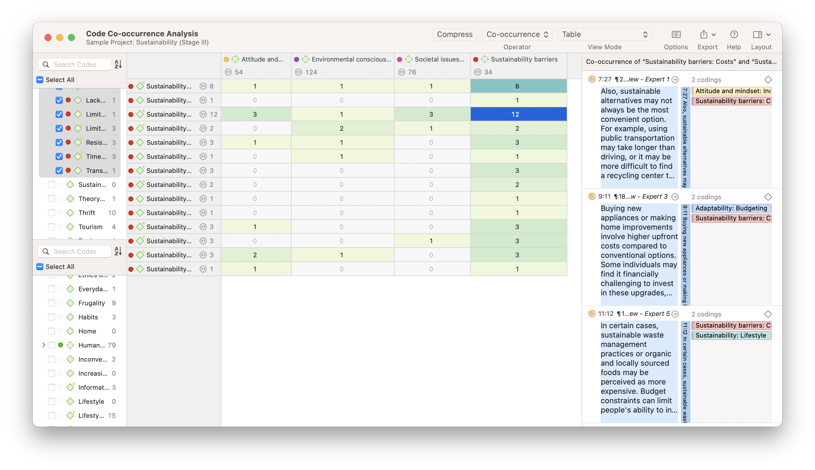
Memos are an important part of any research, which is why ATLAS.ti provides a space separate from your data and codes for research notes and reflection memos. Especially in the social sciences or any field that explores socially constructed concepts, a reflective memo can provide essential documentation of how researchers are involved in data gathering and data interpretation.
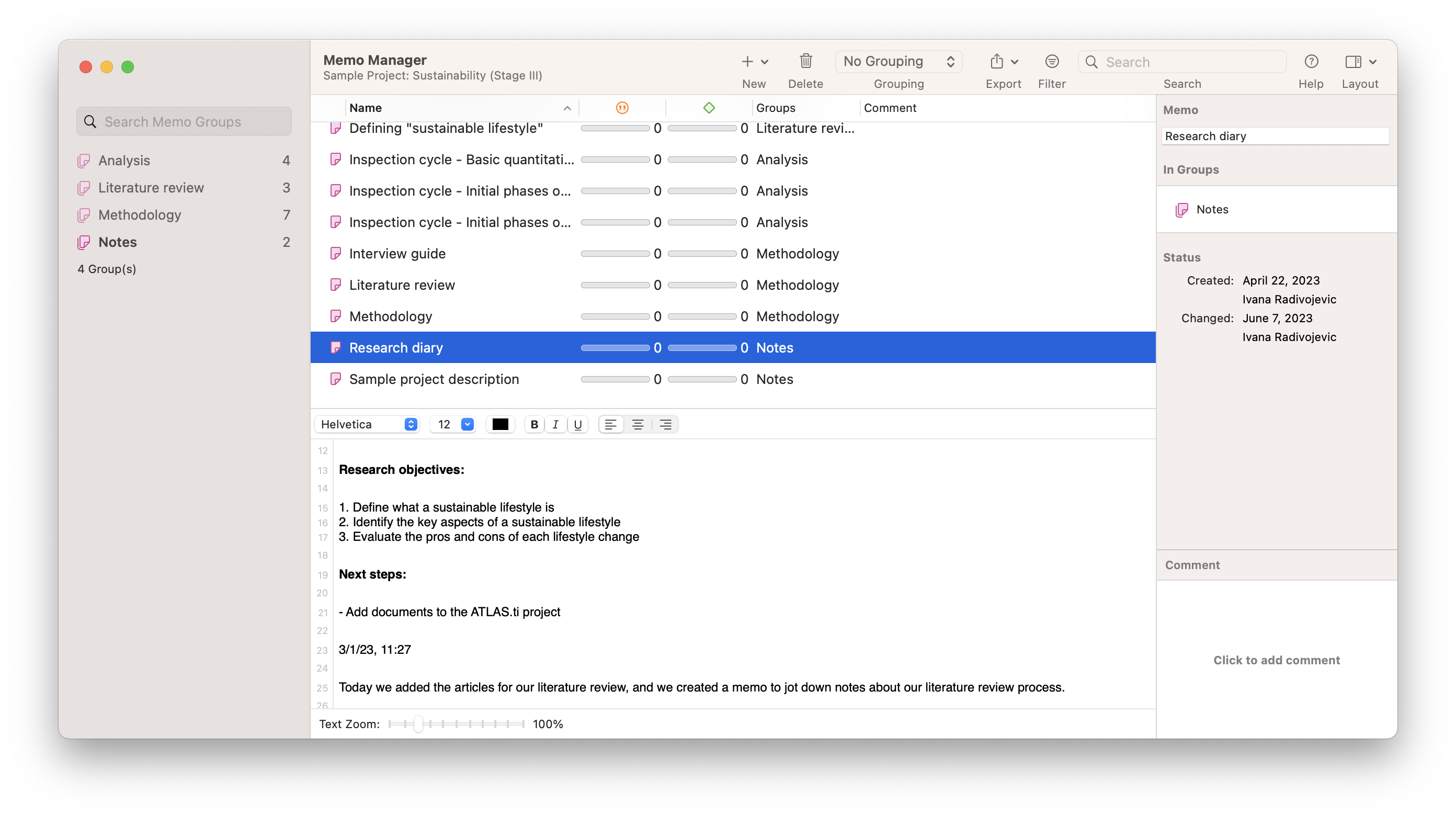
With memos, the steps of analysis can be traced, and the entire process is open to view. Detailed documentation of the data analysis and data interpretation process can also facilitate the reporting and visualization of research when it comes time to share the research with audiences.

In research, the main objective in explicitly conducting and detailing your data interpretation process is to report your research in a manner that is meaningful and persuasive to your audience. Where possible, researchers benefit from visualizing their data interpretation to provide research audiences with the necessary clarity to understand the findings of the research.
Ultimately, the various data analysis processes you employ should lead to some form of reporting where the research audience can easily understand the data interpretation. Otherwise, data interpretation holds no value if it is not understood, let alone accepted, by the research audience.
Data visualization tools in ATLAS.ti
ATLAS.ti has a number of tools that can assist with creating illustrations that contribute to explaining your data interpretation to your research audience.

A TreeMap of your codes can be a useful visualization if you are conducting a thematic analysis of your data. Codes in ATLAS.ti can be marked by different colors, which is illustrative if you use colors to distinguish between different themes in your research. As codes are applied to your data, the more frequently occurring codes take up more space in the TreeMap, allowing you to examine which codes and, by use of colors, which themes are more and less apparent and help you generate theory.
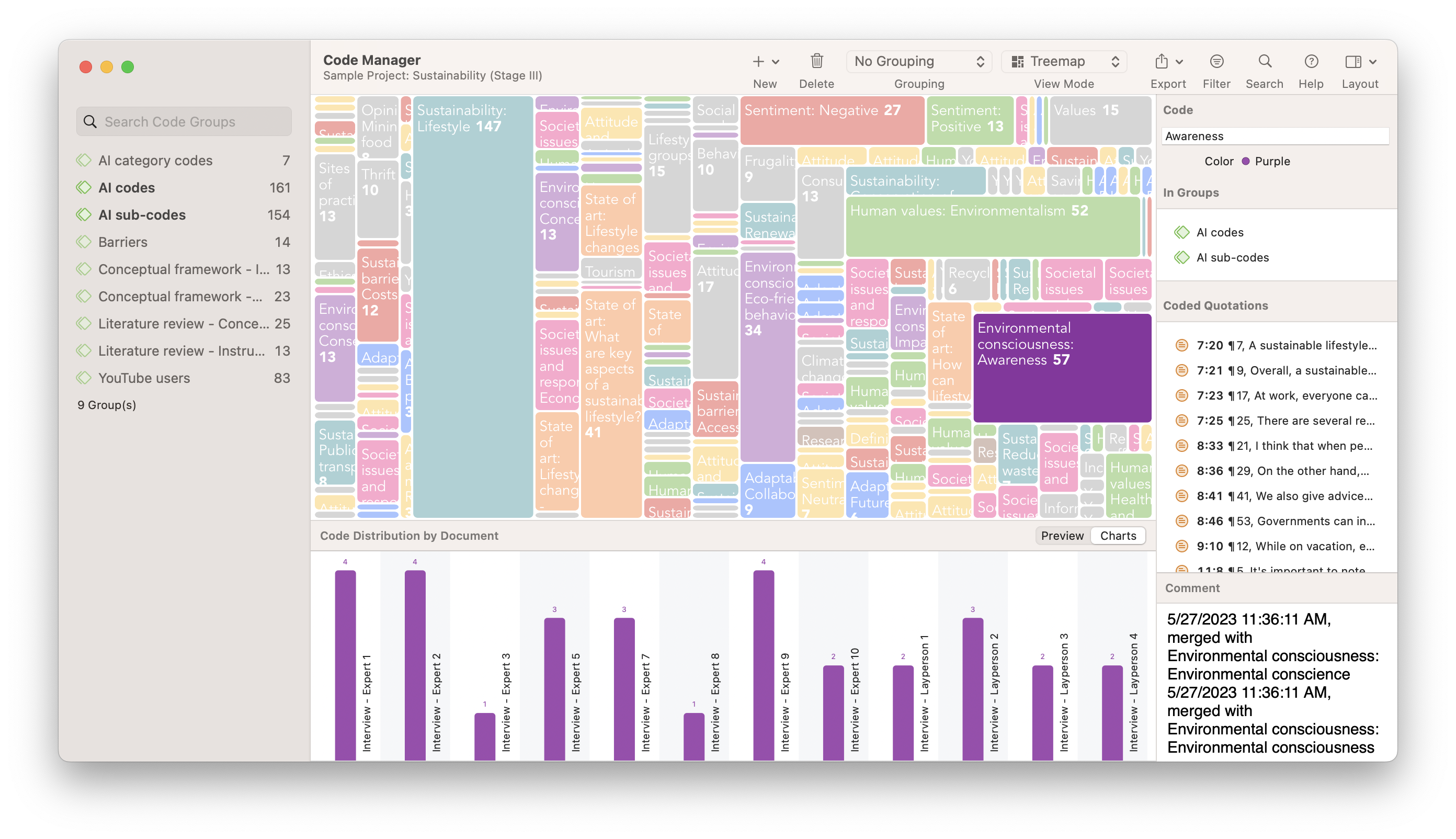
Sankey diagrams
The Code Co-Occurrence and Code-Document Analyses in ATLAS.ti can produce tables, graphs, and also Sankey diagrams, which are useful for visualizing the relative relationships between different codes or between codes and documents. While numerical data generated for tables can tell one story of your data interpretation, the visual information in a Sankey diagram, where higher frequencies are represented by thicker lines, can be particularly persuasive to your research audience.
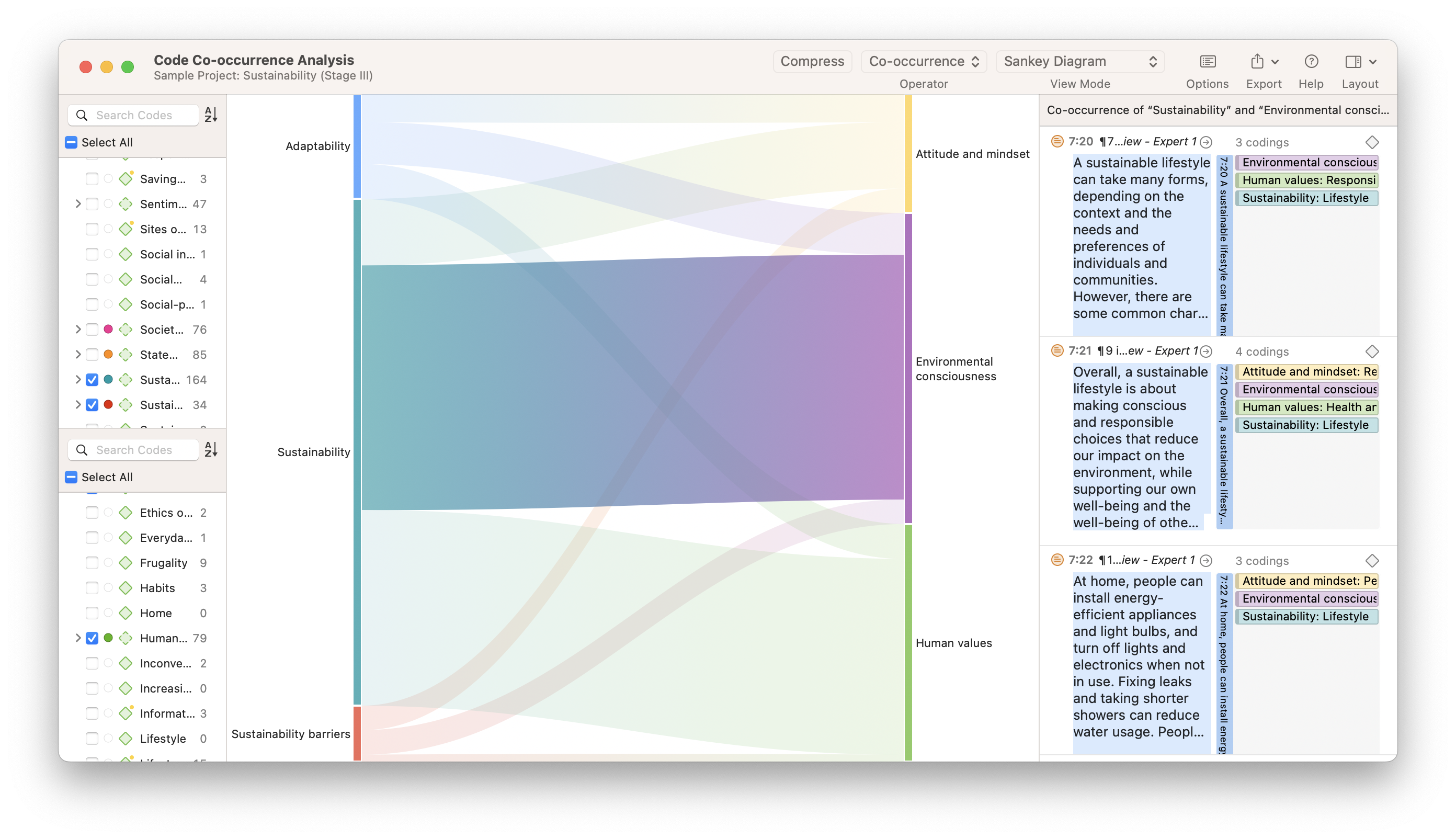
When it comes time to report actionable insights contributing to a theory or conceptualization, you can benefit from a visualization of the theory you have generated from your data interpretation. Networks are made up of elements of your project, usually codes, but also other elements such as documents, code groups, document groups, quotations, and memos. Researchers can then define links between these elements to illustrate connections that arise from your data interpretation.
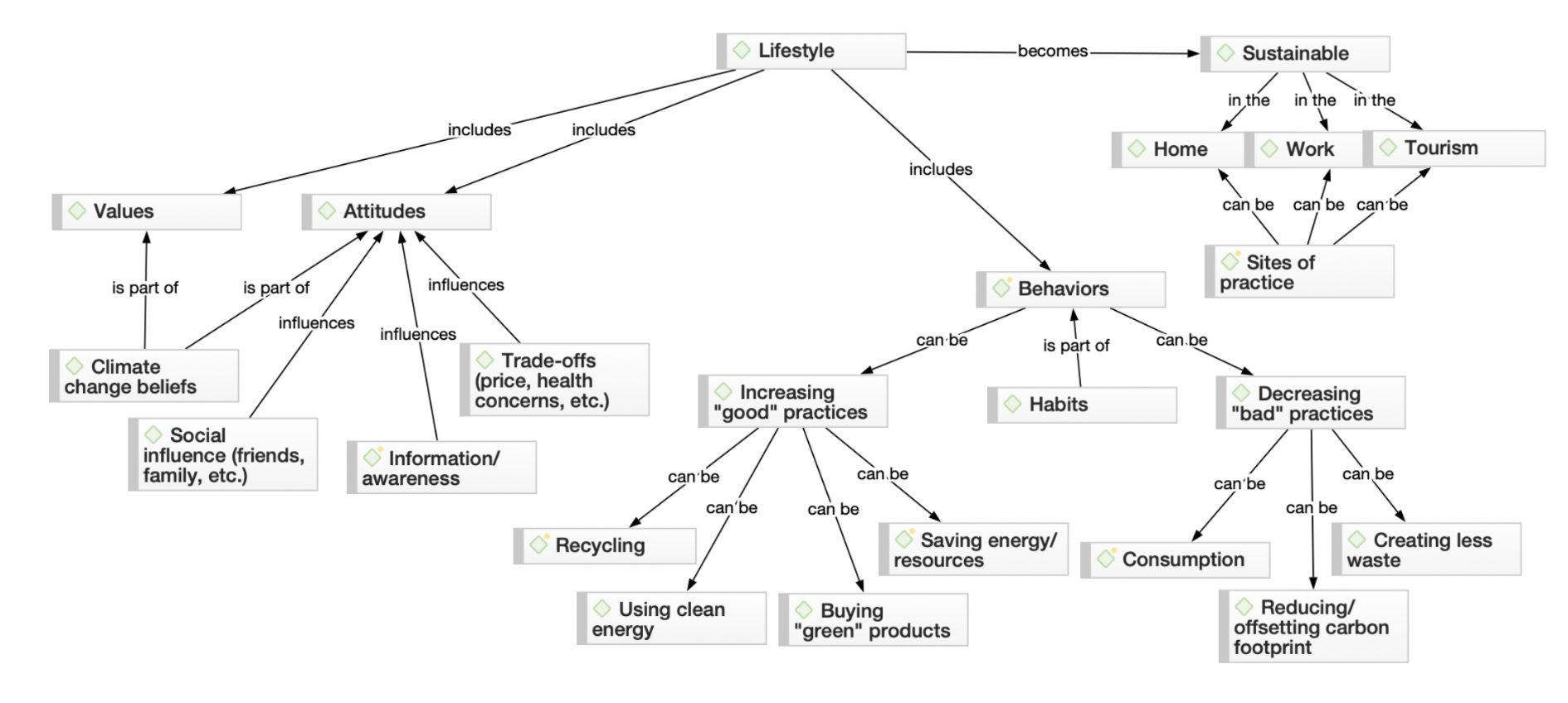
Turn data into insights with ATLAS.ti
Powerful tools to help you interpret data at your fingertips. Click here for a free trial.
- What is Data Interpretation? + [Types, Method & Tools]

- Data Collection
Data interpretation and analysis are fast becoming more valuable with the prominence of digital communication, which is responsible for a large amount of data being churned out daily. According to the WEF’s “A Day in Data” Report , the accumulated digital universe of data is set to reach 44 ZB (Zettabyte) in 2020.
Based on this report, it is clear that for any business to be successful in today’s digital world, the founders need to know or employ people who know how to analyze complex data, produce actionable insights and adapt to new market trends. Also, all these need to be done in milliseconds.
So, what is data interpretation and analysis, and how do you leverage this knowledge to help your business or research? All this and more will be revealed in this article.
What is Data Interpretation?
Data interpretation is the process of reviewing data through some predefined processes which will help assign some meaning to the data and arrive at a relevant conclusion. It involves taking the result of data analysis, making inferences on the relations studied, and using them to conclude.
Therefore, before one can talk about interpreting data, they need to be analyzed first. What then, is data analysis?
Data analysis is the process of ordering, categorizing, manipulating, and summarizing data to obtain answers to research questions. It is usually the first step taken towards data interpretation.
It is evident that the interpretation of data is very important, and as such needs to be done properly. Therefore, researchers have identified some data interpretation methods to aid this process.
What are Data Interpretation Methods?
Data interpretation methods are how analysts help people make sense of numerical data that has been collected, analyzed and presented. Data, when collected in raw form, may be difficult for the layman to understand, which is why analysts need to break down the information gathered so that others can make sense of it.
For example, when founders are pitching to potential investors, they must interpret data (e.g. market size, growth rate, etc.) for better understanding. There are 2 main methods in which this can be done, namely; quantitative methods and qualitative methods .
Qualitative Data Interpretation Method
The qualitative data interpretation method is used to analyze qualitative data, which is also known as categorical data . This method uses texts, rather than numbers or patterns to describe data.
Qualitative data is usually gathered using a wide variety of person-to-person techniques , which may be difficult to analyze compared to the quantitative research method .
Unlike the quantitative data which can be analyzed directly after it has been collected and sorted, qualitative data needs to first be coded into numbers before it can be analyzed. This is because texts are usually cumbersome, and will take more time, and result in a lot of errors if analyzed in their original state. Coding done by the analyst should also be documented so that it can be reused by others and also analyzed.
There are 2 main types of qualitative data, namely; nominal and ordinal data . These 2 data types are both interpreted using the same method, but ordinal data interpretation is quite easier than that of nominal data .
In most cases, ordinal data is usually labeled with numbers during the process of data collection, and coding may not be required. This is different from nominal data that still needs to be coded for proper interpretation.
Quantitative Data Interpretation Method
The quantitative data interpretation method is used to analyze quantitative data, which is also known as numerical data . This data type contains numbers and is therefore analyzed with the use of numbers and not texts.
Quantitative data are of 2 main types, namely; discrete and continuous data. Continuous data is further divided into interval data and ratio data, with all the data types being numeric .
Due to its natural existence as a number, analysts do not need to employ the coding technique on quantitative data before it is analyzed. The process of analyzing quantitative data involves statistical modelling techniques such as standard deviation, mean and median.
Some of the statistical methods used in analyzing quantitative data are highlighted below:
The mean is a numerical average for a set of data and is calculated by dividing the sum of the values by the number of values in a dataset. It is used to get an estimate of a large population from the dataset obtained from a sample of the population.
For example, online job boards in the US use the data collected from a group of registered users to estimate the salary paid to people of a particular profession. The estimate is usually made using the average salary submitted on their platform for each profession.
- Standard deviation
This technique is used to measure how well the responses align with or deviates from the mean. It describes the degree of consistency within the responses; together with the mean, it provides insight into data sets.
In the job board example highlighted above, if the average salary of writers in the US is $20,000 per annum, and the standard deviation is 5.0, we can easily deduce that the salaries for the professionals are far away from each other. This will birth other questions like why the salaries deviate from each other that much.
With this question, we may conclude that the sample contains people with few years of experience, which translates to a lower salary, and people with many years of experience, translating to a higher salary. However, it does not contain people with mid-level experience.
- Frequency distribution
This technique is used to assess the demography of the respondents or the number of times a particular response appears in research. It is extremely keen on determining the degree of intersection between data points.
Some other interpretation processes of quantitative data include:
- Regression analysis
- Cohort analysis
- Predictive and prescriptive analysis
Tips for Collecting Accurate Data for Interpretation
- Identify the Required Data Type
Researchers need to identify the type of data required for particular research. Is it nominal, ordinal, interval, or ratio data ?
The key to collecting the required data to conduct research is to properly understand the research question. If the researcher can understand the research question, then he can identify the kind of data that is required to carry out the research.
For example, when collecting customer feedback, the best data type to use is the ordinal data type . Ordinal data can be used to access a customer’s feelings about a brand and is also easy to interpret.
- Avoid Biases
There are different kinds of biases a researcher might encounter when collecting data for analysis. Although biases sometimes come from the researcher, most of the biases encountered during the data collection process is caused by the respondent.
There are 2 main biases, that can be caused by the President, namely; response bias and non-response bias . Researchers may not be able to eliminate these biases, but there are ways in which they can be avoided and reduced to a minimum.
Response biases are biases that are caused by respondents intentionally giving wrong answers to responses, while non-response bias occurs when the respondents don’t give answers to questions at all. Biases are capable of affecting the process of data interpretation .
- Use Close Ended Surveys
Although open-ended surveys are capable of giving detailed information about the questions and allowing respondents to fully express themselves, it is not the best kind of survey for data interpretation. It requires a lot of coding before the data can be analyzed.
Close-ended surveys , on the other hand, restrict the respondents’ answers to some predefined options, while simultaneously eliminating irrelevant data. This way, researchers can easily analyze and interpret data.
However, close-ended surveys may not be applicable in some cases, like when collecting respondents’ personal information like name, credit card details, phone number, etc.
Visualization Techniques in Data Analysis
One of the best practices of data interpretation is the visualization of the dataset. Visualization makes it easy for a layman to understand the data, and also encourages people to view the data, as it provides a visually appealing summary of the data.
There are different techniques of data visualization, some of which are highlighted below.
Bar graphs are graphs that interpret the relationship between 2 or more variables using rectangular bars. These rectangular bars can be drawn either vertically or horizontally, but they are mostly drawn vertically.
The graph contains the horizontal axis (x) and the vertical axis (y), with the former representing the independent variable while the latter is the dependent variable. Bar graphs can be grouped into different types, depending on how the rectangular bars are placed on the graph.
Some types of bar graphs are highlighted below:
- Grouped Bar Graph
The grouped bar graph is used to show more information about variables that are subgroups of the same group with each subgroup bar placed side-by-side like in a histogram.
- Stacked Bar Graph
A stacked bar graph is a grouped bar graph with its rectangular bars stacked on top of each other rather than placed side by side.
- Segmented Bar Graph
Segmented bar graphs are stacked bar graphs where each rectangular bar shows 100% of the dependent variable. It is mostly used when there is an intersection between the variable categories.
Advantages of a Bar Graph
- It helps to summarize a large data
- Estimations of key values c.an be made at a glance
- Can be easily understood
Disadvantages of a Bar Graph
- It may require additional explanation.
- It can be easily manipulated.
- It doesn’t properly describe the dataset.
A pie chart is a circular graph used to represent the percentage of occurrence of a variable using sectors. The size of each sector is dependent on the frequency or percentage of the corresponding variables.
There are different variants of the pie charts, but for the sake of this article, we will be restricting ourselves to only 3. For better illustration of these types, let us consider the following examples.
Pie Chart Example : There are a total of 50 students in a class, and out of them, 10 students like Football, 25 students like snooker, and 15 students like Badminton.
- Simple Pie Chart
The simple pie chart is the most basic type of pie chart, which is used to depict the general representation of a bar chart.
- Doughnut Pie Chart
Doughnut pie is a variant of the pie chart, with a blank center allowing for additional information about the data as a whole to be included.
- 3D Pie Chart
3D pie chart is used to give the chart a 3D look and is often used for aesthetic purposes. It is usually difficult to reach because of the distortion of perspective due to the third dimension.
Advantages of a Pie Chart
- It is visually appealing.
- Best for comparing small data samples.
Disadvantages of a Pie Chart
- It can only compare small sample sizes.
- Unhelpful with observing trends over time.
Tables are used to represent statistical data by placing them in rows and columns. They are one of the most common statistical visualization techniques and are of 2 main types, namely; simple and complex tables.
- Simple Tables
Simple tables summarize information on a single characteristic and may also be called a univariate table. An example of a simple table showing the number of employed people in a community concerning their age group.
- Complex Tables
As its name suggests, complex tables summarize complex information and present them in two or more intersecting categories. A complex table example is a table showing the number of employed people in a population concerning their age group and sex as shown in the table below.
Advantages of Tables
- Can contain large data sets
- Helpful in comparing 2 or more similar things
Disadvantages of Tables
- They do not give detailed information.
- Maybe time-consuming.
Line graphs or charts are a type of graph that displays information as a series of points, usually connected by a straight line. Some of the types of line graphs are highlighted below.
- Simple Line Graphs
Simple line graphs show the trend of data over time, and may also be used to compare categories. Let us assume we got the sales data of a firm for each quarter and are to visualize it using a line graph to estimate sales for the next year.
- Line Graphs with Markers
These are similar to line graphs but have visible markers illustrating the data points
- Stacked Line Graphs
Stacked line graphs are line graphs where the points do not overlap, and the graphs are therefore placed on top of each other. Consider that we got the quarterly sales data for each product sold by the company and are to visualize it to predict company sales for the next year.
Advantages of a Line Graph
- Great for visualizing trends and changes over time.
- It is simple to construct and read.
Disadvantage of a Line Graph
- It can not compare different variables at a single place or time.
Read: 11 Types of Graphs & Charts + [Examples]
What are the Steps in Interpreting Data?
After data collection, you’d want to know the result of your findings. Ultimately, the findings of your data will be largely dependent on the questions you’ve asked in your survey or your initial study questions. Here are the four steps for accurately interpreting data
1. Gather the data
The very first step in interpreting data is having all the relevant data assembled. You can do this by visualizing it first either in a bar, graph, or pie chart. The purpose of this step is to accurately analyze the data without any bias.
Now is the time to remember the details of how you conducted the research. Were there any flaws or changes that occurred when gathering this data? Did you keep any observatory notes and indicators?
Once you have your complete data, you can move to the next stage
2. Develop your findings
This is the summary of your observations. Here, you observe this data thoroughly to find trends, patterns, or behavior. If you are researching about a group of people through a sample population, this is where you analyze behavioral patterns. The purpose of this step is to compare these deductions before drawing any conclusions. You can compare these deductions with each other, similar data sets in the past, or general deductions in your industry.
3. Derive Conclusions
Once you’ve developed your findings from your data sets, you can then draw conclusions based on trends you’ve discovered. Your conclusions should answer the questions that led you to your research. If they do not answer these questions ask why? It may lead to further research or subsequent questions.
4. Give recommendations
For every research conclusion, there has to be a recommendation. This is the final step in data interpretation because recommendations are a summary of your findings and conclusions. For recommendations, it can only go in one of two ways. You can either recommend a line of action or recommend that further research be conducted.
How to Collect Data with Surveys or Questionnaires
As a business owner who wants to regularly track the number of sales made in your business, you need to know how to collect data. Follow these 4 easy steps to collect real-time sales data for your business using Formplus.
Step 1 – Register on Formplus
- Visit Formplus on your PC or mobile device.
- Click on the Start for Free button to start collecting data for your business.
Step 2 – Start Creating Surveys For Free
- Go to the Forms tab beside your Dashboard in the Formplus menu.
- Click on Create Form to start creating your survey
- Take advantage of the dynamic form fields to add questions to your survey.
- You can also add payment options that allow you to receive payments using Paypal, Flutterwave, and Stripe.
Step 3 – Customize Your Survey and Start Collecting Data
- Go to the Customise tab to beautify your survey by adding colours, background images, fonts, or even a custom CSS.
- You can also add your brand logo, colour and other things to define your brand identity.
- Preview your form, share, and start collecting data.
Step 4 – Track Responses Real-time
- Track your sales data in real-time in the Analytics section.
Why Use Formplus to Collect Data?
The responses to each form can be accessed through the analytics section, which automatically analyzes the responses collected through Formplus forms. This section visualizes the collected data using tables and graphs, allowing analysts to easily arrive at an actionable insight without going through the rigorous process of analyzing the data.
- 30+ Form Fields
There is no restriction on the kind of data that can be collected by researchers through the available form fields. Researchers can collect both quantitative and qualitative data types simultaneously through a single questionnaire.
- Data Storage
The data collected through Formplus are safely stored and secured in the Formplus database. You can also choose to store this data in an external storage device.
- Real-time access
Formplus gives real-time access to information, making sure researchers are always informed of the current trends and changes in data. That way, researchers can easily measure a shift in market trends that inform important decisions.
- WordPress Integration
Users can now embed Formplus forms into their WordPress posts and pages using a shortcode. This can be done by installing the Formplus plugin into your WordPress websites.
Advantages and Importance of Data Interpretation
- Data interpretation is important because it helps make data-driven decisions.
- It saves costs by providing costing opportunities
- The insights and findings gotten from interpretation can be used to spot trends in a sector or industry.
Conclusion
Data interpretation and analysis is an important aspect of working with data sets in any field or research and statistics. They both go hand in hand, as the process of data interpretation involves the analysis of data.
The process of data interpretation is usually cumbersome, and should naturally become more difficult with the best amount of data that is being churned out daily. However, with the accessibility of data analysis tools and machine learning techniques, analysts are gradually finding it easier to interpret data.
Data interpretation is very important, as it helps to acquire useful information from a pool of irrelevant ones while making informed decisions. It is found useful for individuals, businesses, and researchers.
Connect to Formplus, Get Started Now - It's Free!
- data analysis
- data interpretation
- data interpretation methods
- how to analyse data
- how to interprete data
- qualitative data
- quantitative data
- busayo.longe
You may also like:
15 Reasons to Choose Quantitative over Qualitative Research
This guide tells you everything you need to know about qualitative and quantitative research, it differences,types, when to use it, how...
Qualitative vs Quantitative Data:15 Differences & Similarities
Quantitative and qualitative data differences & similarities in definitions, examples, types, analysis, data collection techniques etc.
Collecting Voice of Customer Data: 9 Techniques that Work
In this article, we’ll show you nine(9) practical ways to collect voice of customer data from your clients.
What is a Panel Survey?
Introduction Panel surveys are a type of survey conducted over a long period measuring consumer behavior and perception of a product, an...
Formplus - For Seamless Data Collection
Collect data the right way with a versatile data collection tool. try formplus and transform your work productivity today..
Data Analysis and Interpretation: Revealing and explaining trends
by Anne E. Egger, Ph.D., Anthony Carpi, Ph.D.
Listen to this reading
Did you know that scientists don't always agree on what data mean? Different scientists can look at the same set of data and come up with different explanations for it, and disagreement among scientists doesn't point to bad science.
Data collection is the systematic recording of information; data analysis involves working to uncover patterns and trends in datasets; data interpretation involves explaining those patterns and trends.
Scientists interpret data based on their background knowledge and experience; thus, different scientists can interpret the same data in different ways.
By publishing their data and the techniques they used to analyze and interpret those data, scientists give the community the opportunity to both review the data and use them in future research.
Before you decide what to wear in the morning, you collect a variety of data: the season of the year, what the forecast says the weather is going to be like, which clothes are clean and which are dirty, and what you will be doing during the day. You then analyze those data . Perhaps you think, "It's summer, so it's usually warm." That analysis helps you determine the best course of action, and you base your apparel decision on your interpretation of the information. You might choose a t-shirt and shorts on a summer day when you know you'll be outside, but bring a sweater with you if you know you'll be in an air-conditioned building.
Though this example may seem simplistic, it reflects the way scientists pursue data collection, analysis , and interpretation . Data (the plural form of the word datum) are scientific observations and measurements that, once analyzed and interpreted, can be developed into evidence to address a question. Data lie at the heart of all scientific investigations, and all scientists collect data in one form or another. The weather forecast that helped you decide what to wear, for example, was an interpretation made by a meteorologist who analyzed data collected by satellites. Data may take the form of the number of bacteria colonies growing in soup broth (see our Experimentation in Science module), a series of drawings or photographs of the different layers of rock that form a mountain range (see our Description in Science module), a tally of lung cancer victims in populations of cigarette smokers and non-smokers (see our Comparison in Science module), or the changes in average annual temperature predicted by a model of global climate (see our Modeling in Science module).
Scientific data collection involves more care than you might use in a casual glance at the thermometer to see what you should wear. Because scientists build on their own work and the work of others, it is important that they are systematic and consistent in their data collection methods and make detailed records so that others can see and use the data they collect.
But collecting data is only one step in a scientific investigation, and scientific knowledge is much more than a simple compilation of data points. The world is full of observations that can be made, but not every observation constitutes a useful piece of data. For example, your meteorologist could record the outside air temperature every second of the day, but would that make the forecast any more accurate than recording it once an hour? Probably not. All scientists make choices about which data are most relevant to their research and what to do with those data: how to turn a collection of measurements into a useful dataset through processing and analysis , and how to interpret those analyzed data in the context of what they already know. The thoughtful and systematic collection, analysis, and interpretation of data allow them to be developed into evidence that supports scientific ideas, arguments, and hypotheses .
Data collection, analysis , and interpretation: Weather and climate
The weather has long been a subject of widespread data collection, analysis , and interpretation . Accurate measurements of air temperature became possible in the mid-1700s when Daniel Gabriel Fahrenheit invented the first standardized mercury thermometer in 1714 (see our Temperature module). Air temperature, wind speed, and wind direction are all critical navigational information for sailors on the ocean, but in the late 1700s and early 1800s, as sailing expeditions became common, this information was not easy to come by. The lack of reliable data was of great concern to Matthew Fontaine Maury, the superintendent of the Depot of Charts and Instruments of the US Navy. As a result, Maury organized the first international Maritime Conference , held in Brussels, Belgium, in 1853. At this meeting, international standards for taking weather measurements on ships were established and a system for sharing this information between countries was founded.
Defining uniform data collection standards was an important step in producing a truly global dataset of meteorological information, allowing data collected by many different people in different parts of the world to be gathered together into a single database. Maury's compilation of sailors' standardized data on wind and currents is shown in Figure 1. The early international cooperation and investment in weather-related data collection has produced a valuable long-term record of air temperature that goes back to the 1850s.

Figure 1: Plate XV from Maury, Matthew F. 1858. The Winds. Chapter in Explanations and Sailing Directions. Washington: Hon. Isaac Toucey.
This vast store of information is considered "raw" data: tables of numbers (dates and temperatures), descriptions (cloud cover), location, etc. Raw data can be useful in and of itself – for example, if you wanted to know the air temperature in London on June 5, 1801. But the data alone cannot tell you anything about how temperature has changed in London over the past two hundred years, or how that information is related to global-scale climate change. In order for patterns and trends to be seen, data must be analyzed and interpreted first. The analyzed and interpreted data may then be used as evidence in scientific arguments, to support a hypothesis or a theory .
Good data are a potential treasure trove – they can be mined by scientists at any time – and thus an important part of any scientific investigation is accurate and consistent recording of data and the methods used to collect those data. The weather data collected since the 1850s have been just such a treasure trove, based in part upon the standards established by Matthew Maury . These standards provided guidelines for data collections and recording that assured consistency within the dataset . At the time, ship captains were able to utilize the data to determine the most reliable routes to sail across the oceans. Many modern scientists studying climate change have taken advantage of this same dataset to understand how global air temperatures have changed over the recent past. In neither case can one simply look at the table of numbers and observations and answer the question – which route to take, or how global climate has changed. Instead, both questions require analysis and interpretation of the data.
Comprehension Checkpoint
- Data analysis: A complex and challenging process
Though it may sound straightforward to take 150 years of air temperature data and describe how global climate has changed, the process of analyzing and interpreting those data is actually quite complex. Consider the range of temperatures around the world on any given day in January (see Figure 2): In Johannesburg, South Africa, where it is summer, the air temperature can reach 35° C (95° F), and in Fairbanks, Alaska at that same time of year, it is the middle of winter and air temperatures might be -35° C (-31° F). Now consider that over huge expanses of the ocean, where no consistent measurements are available. One could simply take an average of all of the available measurements for a single day to get a global air temperature average for that day, but that number would not take into account the natural variability within and uneven distribution of those measurements.

Figure 2: Satellite image composite of average air temperatures (in degrees Celsius) across the globe on January 2, 2008 (http://www.ssec.wisc.edu/data/).
Defining a single global average temperature requires scientists to make several decisions about how to process all of those data into a meaningful set of numbers. In 1986, climatologists Phil Jones, Tom Wigley, and Peter Wright published one of the first attempts to assess changes in global mean surface air temperature from 1861 to 1984 (Jones, Wigley, & Wright, 1986). The majority of their paper – three out of five pages – describes the processing techniques they used to correct for the problems and inconsistencies in the historical data that would not be related to climate. For example, the authors note:
Early SSTs [sea surface temperatures] were measured using water collected in uninsulated, canvas buckets, while more recent data come either from insulated bucket or cooling water intake measurements, with the latter considered to be 0.3-0.7° C warmer than uninsulated bucket measurements.
Correcting for this bias may seem simple, just adding ~0.5° C to early canvas bucket measurements, but it becomes more complicated than that because, the authors continue, the majority of SST data do not include a description of what kind of bucket or system was used.
Similar problems were encountered with marine air temperature data . Historical air temperature measurements over the ocean were taken aboard ships, but the type and size of ship could affect the measurement because size "determines the height at which observations were taken." Air temperature can change rapidly with height above the ocean. The authors therefore applied a correction for ship size in their data. Once Jones, Wigley, and Wright had made several of these kinds of corrections, they analyzed their data using a spatial averaging technique that placed measurements within grid cells on the Earth's surface in order to account for the fact that there were many more measurements taken on land than over the oceans.
Developing this grid required many decisions based on their experience and judgment, such as how large each grid cell needed to be and how to distribute the cells over the Earth. They then calculated the mean temperature within each grid cell, and combined all of these means to calculate a global average air temperature for each year. Statistical techniques such as averaging are commonly used in the research process and can help identify trends and relationships within and between datasets (see our Statistics in Science module). Once these spatially averaged global mean temperatures were calculated, the authors compared the means over time from 1861 to 1984.
A common method for analyzing data that occur in a series, such as temperature measurements over time, is to look at anomalies, or differences from a pre-defined reference value . In this case, the authors compared their temperature values to the mean of the years 1970-1979 (see Figure 3). This reference mean is subtracted from each annual mean to produce the jagged lines in Figure 3, which display positive or negative anomalies (values greater or less than zero). Though this may seem to be a circular or complex way to display these data, it is useful because the goal is to show change in mean temperatures rather than absolute values.

Figure 3: The black line shows global temperature anomalies, or differences between averaged yearly temperature measurements and the reference value for the entire globe. The smooth, red line is a filtered 10-year average. (Based on Figure 5 in Jones et al., 1986).
Putting data into a visual format can facilitate additional analysis (see our Using Graphs and Visual Data module). Figure 3 shows a lot of variability in the data: There are a number of spikes and dips in global temperature throughout the period examined. It can be challenging to see trends in data that have so much variability; our eyes are drawn to the extreme values in the jagged lines like the large spike in temperature around 1876 or the significant dip around 1918. However, these extremes do not necessarily reflect long-term trends in the data.
In order to more clearly see long-term patterns and trends, Jones and his co-authors used another processing technique and applied a filter to the data by calculating a 10-year running average to smooth the data. The smooth lines in the graph represent the filtered data. The smooth line follows the data closely, but it does not reach the extreme values .
Data processing and analysis are sometimes misinterpreted as manipulating data to achieve the desired results, but in reality, the goal of these methods is to make the data clearer, not to change it fundamentally. As described above, in addition to reporting data, scientists report the data processing and analysis methods they use when they publish their work (see our Understanding Scientific Journals and Articles module), allowing their peers the opportunity to assess both the raw data and the techniques used to analyze them.
- Data interpretation: Uncovering and explaining trends in the data
The analyzed data can then be interpreted and explained. In general, when scientists interpret data, they attempt to explain the patterns and trends uncovered through analysis , bringing all of their background knowledge, experience, and skills to bear on the question and relating their data to existing scientific ideas. Given the personal nature of the knowledge they draw upon, this step can be subjective, but that subjectivity is scrutinized through the peer review process (see our Peer Review in Science module). Based on the smoothed curves, Jones, Wigley, and Wright interpreted their data to show a long-term warming trend. They note that the three warmest years in the entire dataset are 1980, 1981, and 1983. They do not go further in their interpretation to suggest possible causes for the temperature increase, however, but merely state that the results are "extremely interesting when viewed in the light of recent ideas of the causes of climate change."
- Making data available
The process of data collection, analysis , and interpretation happens on multiple scales. It occurs over the course of a day, a year, or many years, and may involve one or many scientists whose priorities change over time. One of the fundamentally important components of the practice of science is therefore the publication of data in the scientific literature (see our Utilizing the Scientific Literature module). Properly collected and archived data continues to be useful as new research questions emerge. In fact, some research involves re-analysis of data with new techniques, different ways of looking at the data, or combining the results of several studies.
For example, in 1997, the Collaborative Group on Hormonal Factors in Breast Cancer published a widely-publicized study in the prestigious medical journal The Lancet entitled, "Breast cancer and hormone replacement therapy: collaborative reanalysis of data from 51 epidemiological studies of 52,705 women with breast cancer and 108,411 women without breast cancer" (Collaborative Group on Hormonal Factors in Breast Cancer, 1997). The possible link between breast cancer and hormone replacement therapy (HRT) had been studied for years, with mixed results: Some scientists suggested a small increase of cancer risk associated with HRT as early as 1981 (Brinton et al., 1981), but later research suggested no increased risk (Kaufman et al., 1984). By bringing together results from numerous studies and reanalyzing the data together, the researchers concluded that women who were treated with hormone replacement therapy were more like to develop breast cancer. In describing why the reanalysis was used, the authors write:
The increase in the relative risk of breast cancer associated with each year of [HRT] use in current and recent users is small, so inevitably some studies would, by chance alone, show significant associations and others would not. Combination of the results across many studies has the obvious advantage of reducing such random fluctuations.
In many cases, data collected for other purposes can be used to address new questions. The initial reason for collecting weather data, for example, was to better predict winds and storms to help assure safe travel for trading ships. It is only more recently that interest shifted to long-term changes in the weather, but the same data easily contribute to answering both of those questions.
- Technology for sharing data advances science
One of the most exciting advances in science today is the development of public databases of scientific information that can be accessed and used by anyone. For example, climatic and oceanographic data , which are generally very expensive to obtain because they require large-scale operations like drilling ice cores or establishing a network of buoys across the Pacific Ocean, are shared online through several web sites run by agencies responsible for maintaining and distributing those data, such as the Carbon Dioxide Information Analysis Center run by the US Department of Energy (see Research under the Resources tab). Anyone can download those data to conduct their own analyses and make interpretations . Likewise, the Human Genome Project has a searchable database of the human genome, where researchers can both upload and download their data (see Research under the Resources tab).
The number of these widely available datasets has grown to the point where the National Institute of Standards and Technology actually maintains a database of databases. Some organizations require their participants to make their data publicly available, such as the Incorporated Research Institutions for Seismology (IRIS): The instrumentation branch of IRIS provides support for researchers by offering seismic instrumentation, equipment maintenance and training, and logistical field support for experiments . Anyone can apply to use the instruments as long as they provide IRIS with the data they collect during their seismic experiments. IRIS then makes these data available to the public.
Making data available to other scientists is not a new idea, but having those data available on the Internet in a searchable format has revolutionized the way that scientists can interact with the data, allowing for research efforts that would have been impossible before. This collective pooling of data also allows for new kinds of analysis and interpretation on global scales and over long periods of time. In addition, making data easily accessible helps promote interdisciplinary research by opening the doors to exploration by diverse scientists in many fields.
Table of Contents
- Data collection, analysis, and interpretation: Weather and climate
- Different interpretations in the scientific community
- Debate over data interpretation spurs further research
Activate glossary term highlighting to easily identify key terms within the module. Once highlighted, you can click on these terms to view their definitions.
Activate NGSS annotations to easily identify NGSS standards within the module. Once highlighted, you can click on them to view these standards.
Interpreting Data: Creating Meaning
- First Online: 22 April 2021
Cite this chapter

- Graham S. Maxwell 3
Part of the book series: The Enabling Power of Assessment ((EPAS,volume 9))
582 Accesses
Data interpretation is seen as a process of meaning making. This requires attention to the purpose in analysing the data, the kinds of questions asked and by whom, and the kind of data that are needed or available. The relationship between questions and data can be interactive. Data can be aggregated, disaggregated, transformed and displayed in order to reveal patterns, relationships and trends. Different ways of comparing data can be identified—against peers, against standards, against self—and of delving more deeply—through protocol analysis, reason analysis, error analysis, and change analysis. Techniques for analysing group change and growth present various technical challenges and cautions. In particular, value-added measures have been shown to have serious flaws if used for teacher and school evaluation. Data literacy is being given increasing attention as a requirement for successful data interpretation and use, along with associated literacies in educational assessment, measurement, statistics and research. These literacies lack clear definition and elaboration. They also present many challenges for professional development and warrant further research.
This is a preview of subscription content, log in via an institution to check access.
Access this chapter
- Available as PDF
- Read on any device
- Instant download
- Own it forever
- Available as EPUB and PDF
- Durable hardcover edition
- Dispatched in 3 to 5 business days
- Free shipping worldwide - see info
Tax calculation will be finalised at checkout
Purchases are for personal use only
Institutional subscriptions
Coburn and Turner ( 2011 ) noted that ‘a handful of studies do link interventions to context, data use process, and outcomes, providing insight into at least a few possible pathways from intervention to student learning’ (p. 195).
There is a fifth question about implications of the data: how to make things better. Because this question extends beyond the meaning of the data and requires additional considerations, such as curriculum and instruction opportunities, this matter is discussed in Chap. 9 .
The characteristics of QSP, along with other programs of the time, are summarised in Wayman et al. ( 2004 ).
The six challenges are quoted from Mason ( 2002 , p. 6); the comments in parenthesis paraphrase the discussion on each of these challenges.
Lachat ( 2001 ) provides several vignettes on the ways in which data disaggregation assisted schools in revealing false assumptions about what affected low achievement, the effectiveness of special programs, equity for specific groups of students, and consistency of expectations across areas of learning.
Protocol analysis and reason analysis were discussed in Chap. 6 as the third and fourth ways of validating reasoning processes in performance assessments.
In the case of multiple-choice tests this could be accomplished by two-tier items that require a defence of the chosen answer (Griffard & Wandersee, 2001 ; Lin, 2004 ; Tan, Treagust, Goh, & Chia, 2002 ; Treagust, 1995 , 2006 ; Wiggins & McTighe, 1998 ).
In some circumstances, sophisticated statistical methods might be applicable for inserting best estimates of the missing data.
Braun ( 2005 , p. 493) warns that ‘the strength of the correspondence between the evidence from one test and that from another, superficially similar, test is determined by the different aspects of knowledge and skills that the two tests tap, by the amount and quality of the information they provide, and by how well they each match the students’ instructional experiences.’
The choice of common items for linking tests can be problematic, as discussed by Michaelides and Haertel ( 2004 , 2014 ). Feuer, Holland, Green, Bertenthal, & Cadell Hemphill, ( 1999 ) caution that there are serious technical problems to be addressed in linking and equating.
Amrein-Beardsley et al., ( 2013 ) introduce a Special Issue of Education Policy Analysis Archives (Volume 21, Number 4) entitled Value-added: What America’s policymakers need to know and understand .
‘Because true teacher effects might be correlated with the characteristics of the students they teach, current VAM approaches cannot separate any existing contextual effects from these true teacher effects. Existing research is not sufficient for determining the generalizability of this finding or the severity of the actual problems associated with omitted background variables. … [O]ur analysis and simulations demonstrate that VAM based rankings of teachers are highly unstable, and that only large differences in estimated impact are likely to be detectable given the effects of sampling error and other sources of uncertainty. Interpretations of differences among teachers based on VAM estimates should be made with extreme caution’ (McCaffrey et al., 2003 , p. 113).
Huff ( 1954 ) provided the ultimate guide (‘How to lie with statistics’), but he was actually directing his comments at the consumer of statistics, therefore warning against misinterpretation.
The extended version is: ‘Data-literate educators continuously, effectively, and ethically access, act on, and communicate multiple types of data from state, local, classroom, and other sources to improve outcomes for students in a manner appropriate to educators’ professional roles and responsibilities’ (DQC, 2014 , p. 6).
Cowie and Cooper ( 2017 ): ‘Assessment literacy, broadly defined, encompasses how to construct, administer and score reliable student assessments and communicate valid interpretations about student learning, as well as the capacity to integrate assessment into teaching and learning for formative purposes’ (p. 148).
Honig and Venkateswaran ( 2012 ) draw attention to the differences between school and central office use of data, and the interrelationships between the two.
A quite different way of characterising assessment literacy has been expressed in the research literature, one that is located in sociocultural theory. This is less concerned with ‘skills, knowledges and cognitions’ than with social, ethical and collaborative practice. Willis, Adie, & Klenowski, ( 2013 ) define ‘teacher assessment literacies as dynamic social practices which are context dependent and which involve teachers in articulating and negotiating classroom and cultural knowledges [sic] with one another and with learners, in initiation, development and practice of assessment to achieve the learning goals of students’ (p. 241). Their focus is the intersection and interconnection of assessment practice and pedagogical practice, characterised as ‘horizontal discourses,’ which offer no guidance on data literacy, seen as a component of ‘vertical discourses’. Teacher collaboration and communities of practice are reviewed in Chap. 10 .
The fifth skill, instructional decision making, is a step beyond data interpretation per se, and is taken up in Chap. 9 .
Kippers, Poortman, Schildkamp, & Visscher, ( 2018 ) also based their approach to data literacy development on the inquiry cycle. They identify five decision steps: set a purpose; collect data; analyse data; interpret data; and take instructional action. Other formulations of the decision cycle are explored in Chap. 9 .
‘Identify problems’ and ‘frame questions’ are potentially relevant, but are not elaborated in the Gummer and Mandinach ( 2015 ) model.
These are a reinterpretation (reframed and reorganized) of Gummer and Mandinach ( 2015 ) where the elements are presented in the form of a mind map.
This list is a paraphrase of Brookhart ( 2011 ), Table 1, p. 7.
Looney, Cumming, van der Kleij, & Harris, ( 2017 ) propose an extension of the concept of assessment literacy to encompass ‘assessment identity’ with ‘not only a range of assessment strategies and skills, and even confidence and self-efficacy in undertaking assessment , but also the beliefs and feelings about assessment’ (p. 15). They also examine assessment literacy instruments for their theoretical justification and validity (Appendix 2).
DeLuca et al., ( 2016a ) also developed a Classroom Assessment Inventory incorporating these dimensions.
Adelson, J. L., Dickenson, E. R., & Cunningham, B. C. (2016). A multigrade, multiyear statewide examination of reading achievement: Examining variability between districts, schools, and students. Educational Researcher, 45 (4), 258–262. https://doi.org/10.3102/0013189X16649960
Article Google Scholar
Allen, L. K., Likens, A. D., & McNamara, D. S. (2018). Writing flexibility in argumentative essays: A multidimensional analysis. Reading and Writing, 32 , 1607–1634. https://doi.org/10.1007/s11145-018-9921-y
American Educational Research Association, American Psychological Association, & National Council on Measurement in Education. (2014). Standards for educational and psychological testing . American Psychological Association.
Google Scholar
American Federation of Teachers, National Council on Measurement in Education, & National Education Association. (1990). Standards for teacher competence in educational assessment of students . National Council on Measurement in Education.
Amrein-Beardsley, A. (2008). Methodological concerns about the education value-added assessment system. Educational Researcher, 37 (2), 65–75. https://doi.org/10.3102/0013189X08316420
Amrein-Beardsley, A. (2014) . Rethinking value-added models in education . Routledge. https://doi.org/10.4324/9780203409909
Amrein-Beardsley, A., Collins, C., Polasky, S. A., & Sloat, E. F. (2013). Value-added model (VAM) research for educational policy: Framing the issue. Education Policy Analysis Archives, 21 (4). https://doi.org/10.14507/epaa.v21n4.2013
Association for Educational Assessment–Europe. (2012). European framework of standards for educational assessment 1.0 . AEA Europe. https://www.aea-europe.net/wp-content/uploads/2017/07/SW_Framework_of_European_Standards.pdf
Athanases, S. Z., Bennett, L. H., & Wahleithner, J. M. (2013). Fostering data literacy through preservice teacher inquiry in English language arts. The Teacher Educator, 48 (1), 8–28. https://doi.org/10.1080/08878730.2012.740151
Baker, E. (2000). Understanding educational quality: Where validity meets technology (William H. Angoff Memorial Lecture Series). Educational Testing Services. http://files.eric.ed.gov/fulltext/ED449172.pdf
Baker, E. L., Barton, P., Darling-Hammond, L, Haertel, E., Ladd, H. F., Linn, R. L., Ravitch, D., Rothstein, R., Shavelson, R. J., & Shepard, L. A. (2010). Problems with the use of student test scores to evaluate teachers . Economic Policy Institute. http://www.epi.org/publication/bp278/
Bernhardt, V. (1998). Data analysis for comprehensive schoolwide improvement . Eye on Education.
Betebenner, D. (2009). Norm- and criterion-referenced student growth. Educational Measurement: Issues and Practice, 28 (4), 42–51. https://doi.org/10.1111/j.1745-3992.2009.00161.x
Betebenner, D. W., & Linn, R.L. (2010). Growth in student achievement: Issues of measurement, longitudinal data analysis and accountability . Educational Testing Service, K–12 Assessment and Performance Management Center.
Braun, H. I. (2005). Using student progress to evaluate teachers: A primer on value-added models (Policy Information Perspective) . Educational Testing Services.
Braun, H., Chudowski, N., & Koenig, J. (Eds.). (2010). Getting value out of value-added: Report of a workshop . Washington, DC: The National Academies Press.
Brookhart, S. M. (2011). Education knowledge and skills for teachers. Educational Measurement: Issues and Practice, 30 (1), 3–12. https://doi.org/10.1111/j.1745-3992.2010.00195.x
Brown, J., & Duguid, P. (2000). The social life of information . Harvard Business School Press.
Cardozo-Gaibisso, L., Kim, S., & Buxton, C. (2019). Thinking beyond the score: Multidimensional analysis of student performance to inform the next generation of science assessments. Journal of Research in Science Teaching, 57 (6), 1–23. https://doi.org/10.1002/tea.21611
Center for Research on Evaluation Standards and Student Testing. (2004). CRESST Quality School Portfolio System: Reporting on school goals and student achievement [PowerPoint presentation]. http://www.slideserve.com/jana/download-presentation-source
Chappuis, J., Stiggins, R. J., Chappuis, S., & Arter, J. A. (2012). Classroom assessment for student learning: Doing it right—Using it well (2nd ed.). Pearson.
Check, J., & Schutt, R. K. (2012). Research methods in education . SAGE. https://doi.org/10.4135/9781544307725
Chen, E., Heritage, M., & Lee, J. (2005). Identifying students’ learning needs with technology. Journal of Education for Students Placed at Risk, 10 (3), 309–332. https://doi.org/10.1207/s15327671espr1003_6
Chick, H., & Pierce, R. (2013). The statistical literacy needed to interpret school assessment data. Mathematics Teacher Education and Development, 15 (2), 5–26.
Choppin, J. (2002, April 1–5). Data use in practice: Examples from the school level [Conference presentation]. American Educational Research Association Annual Meeting, New Orleans, Louisiana, United States. http://archive.wceruw.org/mps/AERA2002/data_use_in_practice.htm
Christman, J. B., Ebby, C. B., & Edmunds, K. A. (2016). Data use practices for improved mathematics teaching and learning: The importance of productive dissonance and recurring feedback cycles. Teachers College Record, 118 (11), 1–32.
Coburn, C. E., & Talbert, J. E. (2006). Conceptions of evidence use in school districts: Mapping the terrain. American Journal of Education, 112 (4), 469–495. https://doi.org/10.1086/505056
Coburn, C. E., Toure, J., & Yamashita. (2009). Evidence, interpretation, and persuasion: Instructional decision making in the district central office. Teachers College Record, 111 (4), 1115–1161.
Coburn, C. E., & Turner, E. O. (2011). Research on data use: A framework and analysis. Measurement: Interdisciplinary Research and Perspectives, 9 (4), 173–206. https://doi.org/10.1080/15366367.2011.626729
Cohen, L., Manion, L., & Morrison, K. (2011). Research methods in education (7th ed.). Routledge.
Corcoran, S. P. (2010). Can teachers be evaluated by their students’ test scores? Should they be? The use of value-added measures of teacher effectiveness in policy and practice . Annenberg Institute for School Reform at Brown University. https://annenberg.brown.edu/sites/default/files/valueAddedReport.pdf
Cowie, B., & Cooper, B. (2017). Exploring the challenge of developing student teacher data literacy. Assessment in Education: Principles, Policy and Practice, 24 (2), 147–163. https://doi.org/10.1080/0969594X.2016.1225668
Cumming, J., Goldstein, H., & Hand, K. (2020). Enhanced use of educational accountability data to monitor educational progress of Australian students with a focus on indigenous students. Educational Assessment, Evaluation and Accountability, 32 , 29–51. https://doi.org/10.1007/s11092-019-09310-x
Darling-Hammond, L., & Adamson, F. (Eds.). (2014). Beyond the bubble test: How performance assessments support 21st century learning . Wiley. https://doi.org/10.1002/9781119210863
Darling-Hammond, L., Amrein-Beardsley, A., Haertel, E., & Rothstein, J. (2012). Evaluating teacher evaluation. Phi Delta Kappan, 93 (6), 8–15. https://doi.org/10.1177/003172171209300603
Data Quality Campaign. (2014). Teacher data literacy: It’s about time . https://dataqualitycampaign.org/resource/teacher-data-literacy-time/
Datnow, A., & Hubbard, L. (2015). Teachers’ use of assessment data to inform instruction: Lessons from the past and prospects for the future. Teachers College Record, 117 (4), 1–26.
Datnow, A., & Park, V. (2009). School system strategies for supporting data. In T. Kowalski & T. Lasley (Eds.), Handbook of data-based decision making for education (pp. 191–206). Routledge.
DeLuca, C., & Bellara, A. (2013). The current state of assessment education: Aligning policy, standards, and teacher education curriculum. Journal of Teacher Education, 64 (4), 356–372. https://doi.org/10.1177/0022487113488144
DeLuca, C., & Klinger, D. A. (2010). Assessment literacy development: Identifying gaps in teacher education candidates’ learning. Assessment in Education: Principles, Policy & Practice, 17 (4), 419–438. https://doi.org/10.1080/0969594X.2010.516643
DeLuca, C., LaPointe-McEwan, D., & Luhanga, U. (2016a). Approaches to classroom assessment inventory: A new instrument to support teacher assessment literacy. Educational Assessment, 21 (4), 248–266. https://doi.org/10.1080/10627197.2016.1236677
DeLuca, C., LaPointe-McEwan, D., & Luhanga, U. (2016b). Teacher assessment literacy: A review of international standards and measures. Educational Assessment, Evaluation and Accountability, 28 , 251–272. https://doi.org/10.1007/s11092-015-9233-6
Downes, D., & Vindurampulle, O. (2007). Value-added measures for school improvement . Department of Education and Early Childhood Development, Office of Education Policy and Innovation.
Dunlap, K., & Piro, J. S. (2016). Diving into data: Developing the capacity for data literacy in teacher education. Cogent Education, 3 (1). https://doi.org/10.1080/2331186X.2015.1132526
Ericsson, K. A., & Simon, H. A. (1980). Verbal reports as data. Psychological Review, 87 (3), 215–251. https://doi.org/10.1037/0033-295X.87.3.215
Ericsson, K. A., & Simon, H. A. (1984/1993). Protocol analysis: Verbal reports as data . MIT Press. https://doi.org/10.7551/mitpress/5657.001.0001
Feuer, M. J., Holland, P. W., Green, B. F., Bertenthal, M. W., & Cadell Hemphill, F. (Eds.). (1999). Uncommon measures: Equivalence and linking among educational tests . National Academies Press.
Fonseca, M. J., Costa, P. P., Lencastre, L., & Tavares, F. (2012). Multidimensional analysis of high-school students’ perceptions and biotechnology. Journal of Biological Education, 46 (3), 129–139. https://doi.org/10.1080/00219266.2011.634019
Frederiksen, N., Glaser, R., Lesgold, A., & Shafto, M. G. (Eds.). (1990). Diagnostic monitoring of skill and knowledge acquisition . Lawrence Erlbaum Associates.
Gardner J., Harlen W., Hayward L., & Stobart G. (2008). Changing assessment practice: Process, principles and standards . Assessment Reform Group. http://www.aria.qub.ac.uk/JG%20Changing%20Assment%20Practice%20Final%20Final.pdf
Goldstein, H. (2001). Using pupil performance data for judging schools and teachers: Scope and limitations. British Educational Research Journal, 27 (4), 433–422. https://doi.org/10.1080/01411920120071443
Goldstein, H. (2011). Multilevel statistical models (4th ed.). Wiley. https://doi.org/10.1002/9780470973394
Gotch, C. M., & French, B. F. (2014). A systematic review of assessment literacy measures. Educational Measurement: Issues and Practice, 33 (2), 14–18. https://doi.org/10.1111/emip.12030
Graue, E., Delaney, K., & Karch, A. (2013). Ecologies of education quality. Education Policy Analysis Archives, 21 (8). https://doi.org/10.14507/epaa.v21n8.2013
Great Schools Partnership. (2015). The glossary of education reform: Aggregate data . http://edglossary.org/aggregate-data/
Greenberg, J., McKee, A., & Walsh, K. (2013). Teacher prep review: A review of the nation’s teacher preparation programs . National Council on Teacher Quality. https://doi.org/10.2139/ssrn.2353894
Greenberg, J., & Walsh, K. (2012). What teacher preparation programs teach about K–12 assessment: A review . National Council on Teacher Quality. https://www.nctq.org/publications/What-Teacher-Preparation-Programs-Teach-about-K%2D%2D12-Assessment:-A-review
Griffard, P. B., & Wandersee, J. H. (2001). The two-tier instrument on photosynthesis: What does it diagnose? International Journal of Science Education, 23 (10), 1039–1052. https://doi.org/10.1080/09500690110038549
Gummer, E. S., & Mandinach, E. B. (2015). Building a conceptual framework for data literacy. Teachers College Record, 117 (4), 1–22.
Hamilton, L. S., Nussbaum, E. M., & Snow, R. E. (1997). Interview procedures for validating science assessments. Applied Measurement in Education, 10 (2), 181–200. https://doi.org/10.1207/s15324818ame1002_5
Hanushek, E. A., Rivkin, S. G., & Taylor, L. L. (1995). Aggregation bias and the estimated effects of school resources (working paper 397). University of Rochester, Center for Economic Research. https://doi.org/10.3386/w5548
Harris, D. N. (2009). The policy issues and policy validity of value-added and other teacher quality measures. In D. H. Gitomer (Ed.), Measurement issues and assessment for teaching quality (pp. 99–130). Sage. https://doi.org/10.4135/9781483329857.n7
Harris, D. (2011). Value-added measures in education: What every educator needs to know . Harvard Education Press.
Heritage, M., Lee, J., Chen, E., & LaTorre, D. (2005). Upgrading America’s use of information to improve student performance (CSE report 661). National Center for Research on Evaluation, Standards, and Student Testing.
Herman, J., & Gribbons, B. (2001). Lessons learned in using data to support school inquiry and continuous improvement: Final report to the Stuart Foundation (CSE technical report 535). Center for the Study of Evaluation and National Center for Research on Evaluation, Standards, and Student Testing.
Hill, H. C., Kapitula, L. R., & Umland, K. L. (2011). A validity argument approach to evaluating value-added scores. American Educational Research Journal, 48 , 794–831. https://doi.org/10.3102/0002831210387916
Hill, M., Smith, L. F., Cowie, B., & Gunn, A. (2013). Preparing initial primary and early childhood teacher education students to use assessment . Wellington, New Zealand: Teaching and Learning Research Initiative.
Holcomb, E. L. (1999). Getting excited about data: How to combine people, passion, and proof . Corwin Press.
Holloway-Libbell, J., & Amrein-Beardsley, A. (2015). ‘Truths’ devoid of empirical proof: Underlying assumptions surrounding value-added models in teacher evaluation. Teachers College Record , 18008.
Honig, M., & Coburn, C. E. (2005). When districts use evidence for instructional improvement: What do we know and where do we go from here? Urban Voices in Education, 6 , 22–26.
Honig, M. I., & Venkateswaran, N. (2012). School–central office relationships in evidence use: Understanding evidence use as a systems problem. American Journal of Education, 112 (2), 199–222. https://doi.org/10.1086/663282
Huff, D. (1954). How to lie with statistics . Norton.
Hughes, G. (2014). Ipsative assessment: Motivation through marking progress . Palgrave Macmillan. https://doi.org/10.1057/9781137267221
Jimerson, J. B., & Wayman, J. C. (2015). Professional learning for using data: Examining teacher needs and supports. Teachers College Record, 117 (4), 1–36.
Johnson, R. S. (1996). Setting our sights: Measuring equity in school change . Los Angeles: The Achievement Council.
Joint Committee on Standards for Educational Evaluation. (2015). Classroom assessment standards: Practices for PreK-12 teachers . http://www.jcsee.org/the-classroom-assessment-standards-new-standards
Kapler Hewitt, K., & Amrein-Beardsley, A. (Eds.). (2016). Student growth measures in policy and practice: Intended and unintended consequences of high-stakes teacher evaluations . Springer. https://doi.org/10.1057/978-1-137-53901-4
Kersting, N., Chen, M.-K., & Stigler, J. (2013). Value-added teacher estimates as part of teacher evaluations: Exploring the specifications on the stability of teacher value-added scores. Education Policy Analysis Archives, 21 (7). https://doi.org/10.14507/epaa.v21n7.2013
Kippers, W. B., Poortman, C. L., Schildkamp, K., & Visscher, A. J. (2018). Data literacy: What do educators learn and struggle with during a data use intervention? Studies in Educational Evaluation, 56 , 21–31. https://doi.org/10.1016/j.stueduc.2017.11.001
Knapp, M. S., Swinnerton, J. A., Copland, M. A., & Monpas-Huber, J. (2006). Data-informed leadership in education . University of Washington, Center for the Study of Teaching and Policy.
Lachat, M. A. (2001). Data-driven high-school reform: The breaking ranks model . The Northeast and Islands Regional Education Laboratory.
Lachat, M. A., & Williams, M. (1996). Learner-based accountability: Using data to support continuous school improvement . Center for Resource Management.
Lachat, M. A., Williams, M., & Smith, S. C. (2006). Making sense of all your data. Principal Leadership, 7 (2), 16–21.
Leighton, J. P., & Gierl, M. J. (2007). Verbal reports as data for cognitive diagnostic assessment. In J. P. Leighton & M. J. Gierl (Eds.), Cognitive diagnostic assessment for education: Theory and Applications (pp. 146–172). Cambridge University Press. https://doi.org/10.1017/CBO9780511611186
Lem, S., Onghena, P., Verschaffel, L., & Van Dooren, W. (2013). On the misinterpretation of histograms and box plots. Educational Psychology, 33 (2), 155–174. https://doi.org/10.1080/01443410.2012.674006
Levine, D., & Lezotte, L. (1990). Unusually effective schools: A review and analysis of research and practice . Wisconsin center for education research, National Center for Effective Schools Research and Development.
Lin, S.-W. (2004). Development and application of a two-tier diagnostic test for high school students’ understanding of flowering plant growth and development. International Journal of Science and Mathematics Education, 2 , 175–199. https://doi.org/10.1007/s10763-004-6484-y
Linn, R. L. (2016). Test-based accountability . The Gordon Commission on the Future of Assessment in Education. https://www.ets.org/Media/Research/pdf/linn_test_based_accountability.pdf
Looney, A., Cumming, J., van der Kleij, F., & Harris, K. (2017). Reconceptualising the role of teachers as assessors: Teacher assessment identity. Assessment in Education: Principles, Policy & Practice, 25 (5), 442–467. https://doi.org/10.1080/0969594X.2016.1268090
Love, N. (2000). Using data, getting results: Collaborative inquiry for school-based mathematics and science reform . Regional Alliance at TERC.
Magone, M. E., Cai, J., Silver, E. A., & Wang, N. (1994). Validating the cognitive complexity and content quality of a mathematics performance assessment. International Journal of Educational Research, 21 (3), 317–340.
Mandinach, E. B., Friedman, J., & Gummer, E. S. (2014). How can schools of education help to build educators’ capacity to use data? A systematic view of the issue. Teachers College Record, 117 (4), 1–50.
Mandinach, E. B., & Gummer, E. S. (2012). Navigating the landscape of data literacy: It IS complex . WestEd. https://www.wested.org/online_pubs/resource1304.pdf
Mandinach, E. B., & Gummer, E. S. (2013). A systematic view of implementing data literacy in educator preparation. Educational Researcher, 42 (1), 30–37. https://doi.org/10.3102/0013189X12459803
Mandinach, E. B., & Gummer, E. S. (2015). Building a conceptual framework for data literacy. Teachers College Record, 117 (4), 1–22.
Mandinach, E. B., & Gummer, E. S. (2016). Every teacher should succeed with data literacy. Phi Delta Kappan, 97 (8), 43–46. https://doi.org/10.1177/0031721716647018
Mandinach, E. B., & Honey, M. (2008). Data-driven decision making: An introduction. In E. B. Mandinach & M. Honey (Eds.), Data-driven school improvement: Linking data and learning (pp. 1–9). Teachers College Press.
Mason, S. (2002, April 1–5). Turning data into knowledge: Lessons from six Milwaukee Public Schools [Conference presentation]. American Educational Research Association Annual Meeting, New Orleans, Louisiana, United States. http://archive.wceruw.org/mps/AERA2002/Mason%20AERA%202002%20QSP%20Symposium%20Paper.pdf
McCaffrey, D. F., Lockwood, J. R., Koretz, D. M., & Hamilton, L. (2003). Evaluating value-added models for teacher accountability . Rand. https://doi.org/10.1037/e658712010-001
McCaffrey, D. F., Lockwood, J. R., Koretz, D., Louis, T. A., & Hamilton, L. (2004). Let’s see more empirical studies on value-added modelling of teacher effects: A reply to Raudenbush, Ruin, Stuart and Zanutto, and Rechase. Journal of Educational and Behavioral Statistics, 29 (1), 139–143. https://doi.org/10.3102/10769986029001139
Means, B., Chen, E., DeBarger, A., & Padilla, C. (2011). Teachers’ ability to use data to inform instructional challenges and supports . U.S. Department of Education, Office of Planning, Evaluation and Policy Development.
Means, B., Padilla, C., DeBarger, A., & Bakia, M. (2009). Implementing data-informed decision making in schools: Teacher access, supports and use . U.S. Department of Education.
Mertler, C. A. (2018). Norm-referenced interpretation. In B. B. Frey (Ed.), The SAGE encyclopedia of educational research, measurement, and evaluation (pp. 1161–1163). Sage. https://doi.org/10.4135/9781506326139
Messick, S. (1989). Validity. In R. L. Linn (Ed.), Educational measurement (3rd ed., pp. 13–103). Macmillan.
Messick, S. (1996). Validity of performance assessment. In G. Philips (Ed.), Technical issues in large-scale performance assessment (pp. 1–18). National Center for Educational Statistics.
Michael and Susan Dell Foundation. (2016a). Boston teacher residency . https://www.msdf.org/wp-content/uploads/2019/06/MSDF_teacherprep_BTR-1.pdf
Michael and Susan Dell Foundation. (2016b). Data-literate teachers: Insights from pioneer programs . https://www.msdf.org/wp-content/uploads/2019/06/MSDF_teacherprep.pdf
Michaelides, M. P., & Haertel, E. H. (2004). Sampling of common items: An unrecognized source of error in test equating . Los Angeles: Center for Research on Evaluation Standards and Student Testing.
Michaelides, M. P., & Haertel, E. H. (2014). Sampling of common items as an unrecognized source of error in test equating: A bootstrap approximation assuming random sampling of common items. Applied Measurement in Education, 27 (1), 46–57. https://doi.org/10.1080/08957347.2013.853069
Michigan Assessment Consortium. (2020). Assessment literacy standards . https://www.michiganassessmentconsortium.org/assessment-literacy-standards/
Moss, P. A. (2012). Exploring the macro-micro dynamic in data use practice. American Journal of Education, 118 (2), 223–232. https://doi.org/10.1086/663274
Muijs, D. (2006). Measuring teacher effectiveness: Some methodological reflection. Educational Research and Evaluation, 12 (1), 53–74. https://doi.org/10.1080/13803610500392236
Newton, X., Darling-Hammond, L., Haertel, E., & Thomas, E. (2010). Value-added modeling of teacher effectiveness: An exploration of stability across models and contexts. Education Policy Analysis Archives, 18 (23). https://doi.org/10.14507/epaa.v18n23.2010
Nickodem, K., & Rodriguez, M. C. (2018). Criterion-referenced interpretation. In B. B. Frey (Ed.), The SAGE encyclopedia of educational research, measurement, and evaluation (pp. 426–428). SAGE. https://doi.org/10.4135/9781506326139
O’Day, J. (2002). Complexity, accountability, and school improvement. Harvard Educational Review, 72 (3), 293–329. https://doi.org/10.17763/haer.72.3.021q742t8182h238
Organisation for Economic Development and Cooperation. (2008). Measuring improvement in learning outcomes: Best practices to assess the value-added of schools . https://doi.org/10.1787/9789264050259-en
Papay, J. P. (2011). Different tests, different answers. American Educational Research Journal, 48 (1), 163–193. https://doi.org/10.3102/0002831210362589
Pellegrino, J. W., Chudowsky, N., & Glaser, R. (Eds.). (2001). Knowing what students know: The science of design and educational assessment . National Academies Press.
Phillips, D. C. (2007). Adding complexity: Philosophical perspectives on the relationship between evidence and policy. Yearbook of the National Society for the Study of Education, 106 (1), 376–402. https://doi.org/10.1111/j.1744-7984.2007.00110.x
Pierce, R., & Chick, H. (2013). Workplace statistical literacy for teachers: Interpreting box plots. Mathematics Education Research Journal, 25 (1), 189–205. https://doi.org/10.1007/s13394-012-0046-3
Pierce, R., Chick, H., & Gordon, I. (2013). Teachers’ perceptions of factors influencing their engagement with statistical reports on student data. Australian Journal of Education, 57 (3), 237–255. https://doi.org/10.1177/0004944113496176
Pierce, R., Chick, H., Watson, J., Magdalena, L., & Dalton, M. (2014). A statistical literacy hierarchy for interpreting educational system data. Australian Journal of Education, 58 (2), 195–217. https://doi.org/10.1177/0004944114530067
Piro, J. S., & Hutchinson, C. J. (2014). Using data chat to teach instructional interventions: Student perceptions of data literacy in an assessment course. The New Educator, 10 (2), 95–111. https://doi.org/10.1080/1547688X.2014.898479
Popham, W. J. (2009). Assessment literacy for teachers: Faddish or fundamental? Theory Into Practice, 48 (1), 4–11. https://doi.org/10.1080/00405840802577536
Popham, W. J. (2014). Classroom assessment: What teachers need to know (7th ed.). Pearson.
Raudenbush, S. W. (2004). What are value-added models estimating and what does this imply for statistical practice? Journal of Educational and Behavioral Statistics, 29 (1), 121–129. https://doi.org/10.3102/10769986029001121
Reckase, M. D. (2004). The real world is more complicated than we would like. Journal of Educational and Behavioral Statistics, 29 (1), 117–120. https://doi.org/10.3102/10769986029001117
Reeves, T. D., & Honig, S. L. (2015). A classroom data literacy intervention for pre-service teachers. Teaching and Teacher Education, 50 , 90–101. https://doi.org/10.1016/j.tate.2015.05.007
Rubin, D. B., Stuart, E. A., & Zanutto, E. L. (2004). A potential outcomes view of value-added assessment in education. Journal of Educational and Behavioral Statistics, 29 (1), 103–116. https://doi.org/10.3102/10769986029001103
Schmidt, W. H., Houang, R. T., & McKnight, C. C. (2005). Value-added research: Right idea but wrong solution? In R. Lissitz (Ed.), Value-added models in education: Theory and applications (pp. 145–165). Maple Grove: JAM Press.
Schochet, P. Z., & Chiang, H. S. (2010). Error rates in measuring teacher and school performance based on student test score gains . U.S. Department of Education, Institute of Education Sciences, National Center for Education Evaluation and Regional Assistance.
Shepard, L. A. (2013). Validity for what purpose? Teachers College Record, 115 (9), 1–15.
Sloane, F. C., Oloff-Lewis, J., & Kim, S. H. (2013). Value-added models of teacher and school effectiveness in Ireland: Wise or otherwise? Irish Educational Studies, 32 (1), 37–67. https://doi.org/10.1080/03323315.2013.773233
Spillane, J. P., & Miele, D. B. (2007). Evidence in practice: A framing of the terrain. Yearbook of the National Society for the Study of Evidence, 106 (1), 46–73. https://doi.org/10.1111/j.1744-7984.2007.00097.x
Tan, D. K.-C., Treagust, D. F., Goh, N.-K., & Chia, L.-S. (2002). Development and application of a two-tier multiple-choice diagnostic instrument to assess high school students’ understanding of inorganic qualitative analysis. Journal of Research in Science Teaching, 39 (4), 283–301. https://doi.org/10.1002/tea.10023
Treagust, D. F. (1995). Diagnostic assessment of students’ science concepts. In S. Glynn & R. Duit (Eds.), Learning science in the schools: Research reforming practice (pp. 327–346). Lawrence Erlbaum Associates.
Treagust, D. F. (2006). Diagnostic assessment in science as a means to improving teaching, learning and retention. In Uniserve Science Assessment Symposium Proceedings. https://core.ac.uk/download/pdf/229410386.pdf
Tufte, E. R. (1983). The visual display of quantitative information . Graphics Press.
Tufte, E. R. (1990). Envisioning information . Graphics Press.
Tufte, E. R. (1997). Visual explanations . Graphics Press.
Tversky, B. (1997). Cognitive principles of graphic displays . AAAI Technical Report FS-97-03, pp. 116–124. https://www.aaai.org/Papers/Symposia/Fall/1997/FS-97-03/FS97-03-015.pdf
United Kingdom Department of Education. (2016). Eliminating unnecessary workload associated with data management: Report of the Independent Teacher Workload Review Group. Government Publications.
van Barneveld, C. (2008). Using data to improve student achievement (What Works: Research into Practice, Research Monograph #15). http://www.edu.gov.on.ca/eng/literacynumeracy/inspire/research/Using_Data.pdf
Volante, L., & Fazio, X. (2007). Exploring teacher candidates’ assessment literacy: Implications for teacher education reform and professional development. Canadian Journal of Education, 30 (3), 749–770. https://doi.org/10.2307/20466661
Wayman, J. C., & Jimerson, J. B. (2014). Teacher needs for data-related professional learning. Studies in Educational Evaluation, 42 , 25–34. https://doi.org/10.1016/j.stueduc.2013.11.001
Wayman, J. C., Stringfield, S., & Yakimowski, M. (2004). Software enabling school improvement through analysis of student data (report no. 67). CRESPAR/Johns Hopkins University.
Wiggins, G., & McTighe, J. (1998). Understanding by design . Association for Supervision and Curriculum Development.
Willis, J., Adie, L., & Klenowski, V. (2013). Conceptualising teachers’ assessment literacies in an era of curriculum and assessment reform. Australian Educational Researcher, 40 , 241–256. https://doi.org/10.1007/s13384-013-0089-9
Yen, W. M. (2007). Vertical scaling and no child left behind. In N. J. Dorans, M. Pommerich, & P. W. Holland (Eds.), Linking and aligning scores and scales (pp. 273–283). Springer. https://doi.org/10.1007/978-0-387-49771-6_15
Download references
Author information
Authors and affiliations.
Institute for Learning Sciences and Teacher Education, Australian Catholic University, Brisbane, QLD, Australia
Graham S. Maxwell
You can also search for this author in PubMed Google Scholar
Rights and permissions
Reprints and permissions
Copyright information
© 2021 Springer Nature Switzerland AG
About this chapter
Maxwell, G.S. (2021). Interpreting Data: Creating Meaning. In: Using Data to Improve Student Learning. The Enabling Power of Assessment, vol 9. Springer, Cham. https://doi.org/10.1007/978-3-030-63539-8_8
Download citation
DOI : https://doi.org/10.1007/978-3-030-63539-8_8
Published : 22 April 2021
Publisher Name : Springer, Cham
Print ISBN : 978-3-030-63537-4
Online ISBN : 978-3-030-63539-8
eBook Packages : Education Education (R0)
Share this chapter
Anyone you share the following link with will be able to read this content:
Sorry, a shareable link is not currently available for this article.
Provided by the Springer Nature SharedIt content-sharing initiative
- Publish with us
Policies and ethics
- Find a journal
- Track your research

Research Methods
- Getting Started
- What is Research Design?
- Research Approach
- Research Methodology
- Data Collection
- Data Analysis & Interpretation
- Population & Sampling
- Theories, Theoretical Perspective & Theoretical Framework
- Useful Resources
Further Resources

Data Analysis & Interpretation
- Quantitative Data
Qualitative Data
- Mixed Methods
You will need to tidy, analyse and interpret the data you collected to give meaning to it, and to answer your research question. Your choice of methodology points the way to the most suitable method of analysing your data.

If the data is numeric you can use a software package such as SPSS, Excel Spreadsheet or “R” to do statistical analysis. You can identify things like mean, median and average or identify a causal or correlational relationship between variables.
The University of Connecticut has useful information on statistical analysis.
If your research set out to test a hypothesis your research will either support or refute it, and you will need to explain why this is the case. You should also highlight and discuss any issues or actions that may have impacted on your results, either positively or negatively. To fully contribute to the body of knowledge in your area be sure to discuss and interpret your results within the context of your research and the existing literature on the topic.
Data analysis for a qualitative study can be complex because of the variety of types of data that can be collected. Qualitative researchers aren’t attempting to measure observable characteristics, they are often attempting to capture an individual’s interpretation of a phenomena or situation in a particular context or setting. This data could be captured in text from an interview or focus group, a movie, images, or documents. Analysis of this type of data is usually done by analysing each artefact according to a predefined and outlined criteria for analysis and then by using a coding system. The code can be developed by the researcher before analysis or the researcher may develop a code from the research data. This can be done by hand or by using thematic analysis software such as NVivo.
Interpretation of qualitative data can be presented as a narrative. The themes identified from the research can be organised and integrated with themes in the existing literature to give further weight and meaning to the research. The interpretation should also state if the aims and objectives of the research were met. Any shortcomings with research or areas for further research should also be discussed (Creswell,2009)*.
For further information on analysing and presenting qualitative date, read this article in Nature .
Mixed Methods Data
Data analysis for mixed methods involves aspects of both quantitative and qualitative methods. However, the sequencing of data collection and analysis is important in terms of the mixed method approach that you are taking. For example, you could be using a convergent, sequential or transformative model which directly impacts how you use different data to inform, support or direct the course of your study.
The intention in using mixed methods is to produce a synthesis of both quantitative and qualitative information to give a detailed picture of a phenomena in a particular context or setting. To fully understand how best to produce this synthesis it might be worth looking at why researchers choose this method. Bergin**(2018) states that researchers choose mixed methods because it allows them to triangulate, illuminate or discover a more diverse set of findings. Therefore, when it comes to interpretation you will need to return to the purpose of your research and discuss and interpret your data in that context. As with quantitative and qualitative methods, interpretation of data should be discussed within the context of the existing literature.
Bergin’s book is available in the Library to borrow. Bolton LTT collection 519.5 BER
Creswell’s book is available in the Library to borrow. Bolton LTT collection 300.72 CRE
For more information on data analysis look at Sage Research Methods database on the library website.
*Creswell, John W.(2009) Research design: qualitative, and mixed methods approaches. Sage, Los Angeles, pp 183
**Bergin, T (2018), Data analysis: quantitative, qualitative and mixed methods. Sage, Los Angeles, pp182
- << Previous: Data Collection
- Next: Population & Sampling >>
- Last Updated: Sep 7, 2023 3:09 PM
- URL: https://tudublin.libguides.com/research_methods
Data Interpretation: Definition, Importance, and Processes

Susanne Morris

Many investors and organizations alike rely on data to enrich their decision-making process. From development to sales, quality data insights can provide professionals with insights into every aspect of their business operations. While this may seem rather straightforward, there are quite a few processes that must be followed so you can utilize data’s full potential. This is where data interpretation comes in.
What is data interpretation?
Ultimately, data interpretation is a data review process that utilizes analysis, evaluation, and visualization to provide in-depth findings to enhance data-driven decision-making. Further, there are many steps involved in data interpretation, as well as different types of data and data analysis processes that influence the larger data interpretation process. This article will explain the different data interpretation methods, the data interpretation process, and its benefits. Firstly, let’s start with an overview of data interpretation and its importance.
Why is data interpretation important?
The importance of data interpretation is not far from the importance of other data processes. Much like implementing data normalization and understanding data quality , proper data interpretation offers real-time solutions and provides more in-depth insights than without it. Particularly, data interpretation can improve data identification, discover hidden correlations between datasets, find data outliers, and even help forecast trends .
Additionally, proper implementation of data interpretation offers immense benefits such as cost efficiency, enhanced decision making, and improved AI predictions. Namely, in a Business Intelligence survey, it was reported that companies that implemented data analysis and interpretation from big data datasets saw a ten percent reduction in costs .
While the importance of data interpretation is undeniable, it is significant to note that this process is no easy feat. To unlock the full potential of your data, you must integrate your data interpretation process into your workflow in its entirety. So what is that process? Let’s take a closer look.

The data interpretation process
Data interpretation is a five-step process, with the primary step being data analysis. Without data analysis, there can be no data interpretation. In addition to its importance, the analysis portion of data interpretation, which will be touched on later on includes two different approaches: qualitative analysis and quantitative analysis.
Qualitative analysis
Qualitative analysis is defined as examining and explaining non-quantifiable data through a subjective lens. Further, in terms of data interpretation, qualitative analysis is the process of analyzing categorical data (data that cannot be represented numerically) while applying a contextual lens. Data that cannot be represented numerically includes information such as observations, documentation, and questionnaires.
Ultimately, this data type is analyzed with a contextual lens that accounts for biases, emotions, behaviors, and more. A company review, for instance, accounts for human sentiment, narrative, and previous behaviors during analysis, helping summarize large amounts of quantitative data for further analysis. Due to the personable nature of qualitative analysis, there are a variety of techniques involved in collecting this data including interviews, questionnaires, and information exchanges. Not unlike many lead generation techniques, companies often offer free resources in exchange for information in the form of qualitative data. In practice, for example, companies offer free quality resources such as e-books in exchange for completing product or demographic surveys.
Quantitative analysis
On the other hand, quantitative analysis refers to the examination and explanation of numerical values through a statistical lens. Similarly, with regard to data interpretation, quantitative analysis involves analyzing numerical data that can be then applied to statistical modeling for predictions.
Typically, this type of analysis involves the collection of massive amounts of numerical data that are then analyzed mathematically to produce more conclusive results such as mean, standard deviation, median, and ratios. Similar to the qualitative process, the collection of this quantitative data can involve a variety of different processes. For example, web scraping is a common extraction technique used to collect public online quantitative and qualitative data. In the same way web scraping can be used to extract quantitative data, such as social sentiment, it can also be used to extract numerical data, such as financial data.
If you're looking for data to identify business opportunities, you can perform both types of analysis with Coresignal's raw data.
How to interpret data
Now that we’ve examined the two types of analysis used in the data interpretation process, we can take a closer look at the interpretation process from beginning to end. The five key steps involved in the larger data interpretation process include baseline establishment, data collection, interpretation (qualitative or quantitative analysis), visualization, and reflection. Let’s take a look at each of these steps.
1. Baseline establishment
Similar to the first step when conducting a competitive analysis, it is important to establish your baseline when conducting data interpretation. This can include setting objectives and outlining long-term and short-term goals that will be directly affected by any actions that result from your data interpretation. For example, investors utilizing data interpretation may want to set goals regarding the ROI of companies they are evaluating. It is important to note that this step also includes the determination of which data type you wish to analyze and interpret.
2. Data collection
Now that a baseline is established and the goals of your data interpretation process are known, you can start collecting data. As previously mentioned, the data collection process includes two major collecting types: web scraping and information exchange. Both of these methods are successful at collecting both qualitative and quantitative data. However, depending on the scope of your data interpretation process, you most likely will only require one method.
For example, if you are looking for specific information within a very particular demographic, you will want to target particular attributes within the larger demographic you are interested in. Particularly, let’s say you want to collect sentiment surrounding an application used by a particular job type; you will want to target individuals with a specific job type attribute and utilize information exchange.
Both of these collection methods can be quite extensive, and for that reason, you may want to enrich your data collection or even fully utilize high-quality data from a data provider . Notably, once your data is collected, you must clean and organize your data before you can proceed to analysis. This can be achieved through data cleansing and data normalization processes.
3. Interpretation (qualitative or quantitative)
This step is arguably the most crucial one in the data interpretation process, and it involves the analysis of the data you’ve collected. This is where your decision to conduct a qualitative or quantitative analysis comes into play.
Qualitative analysis will require you to use a more subjective lens. If you are using AI-based data analysis tools, extensive “coding” will be necessary so that the data can be understood subjectively as sentiment experienced by individuals that cannot be defined numerically.
On the other hand, qualitative analysis requires that the data be analyzed through a numerical and mathematical approach. As previously mentioned, raw numerical data will be analyzed, resulting in mean, standard deviation, and ratios, which can then be analyzed further via statistical modeling to better understand and predict behaviors.
4. Visualization
When your analysis is complete, you can now start to visualize your data and draw insights from various perspectives. Today, many companies have implemented “dashboards” as a part of the visualization stage. Dashboards essentially provide you with quick insights via programmable algorithms. Even without dashboards formatting your data for visualization is relatively straightforward. To do this, you must input and format your data into a format that supports visualization. Some of the more common visualization formats include:
- Scatter plots
- Line graphs
5. Reflection
Lastly, once you have created adequate visualization types that meet your previously decided objectives, you can reflect. While a rather simple process, relative to the earlier steps, the reflection process can make or break your data interpretation process. During this step, you should reflect on the data analysis process as a whole, look for hidden correlations, AND identify outliers or errors that may have affected your visualization charts (but could have been missed during the data cleansing stage). It is crucial that during this step you differentiate between correlation and causation, identify bias, and take note of any missed insights.

Wrapping up
In all, data interpretation is an extremely important part of data-driven decision-making and should be done regularly as a part of a larger iterative interpretation process. Investors, developers, and sales and acquisition alike can find hidden insights from regularly performed data interpretation. It is what you do with those insights that bring your company success.
Frequently asked questions
Qualitative data interpretation is the process of analyzing categorical data (data that cannot be represented numerically, such as observations, documentation, and questionnaires) through a contextual lens.
Quantitative data interpretation refers to the examination and explanation of numerical data through a statistical lens.
There are five main steps in data interpretation: baseline data establishment (similar to data discovery ), data collection, data interpretation, data visualization, and reflection.
Related articles

Data Wrangling: Benefits, Processes, and Application in AI
Data wrangling is the process of cleaning, transforming, and organizing raw data. This article explores its significance, benefits, methods, and application in AI and machine learning.
10 Most Reliable B2C and B2B Lead Generation Databases
Not all lead databases are created equal. Some are better than others, and knowing how to pick the right one is key. A superior database provides continuously updated and verified data.
It’s a (Data) Match! Data Matching as a Business Value
With the amount of business data growing, more and more options to categorize it appear, resulting in many datasets. Unfortunately, without proper data matching, much business value is lost in between the datasets, forever hidden, and forever unreclaimed.
- Games & Quizzes
- History & Society
- Science & Tech
- Biographies
- Animals & Nature
- Geography & Travel
- Arts & Culture
- On This Day
- One Good Fact
- New Articles
- Lifestyles & Social Issues
- Philosophy & Religion
- Politics, Law & Government
- World History
- Health & Medicine
- Browse Biographies
- Birds, Reptiles & Other Vertebrates
- Bugs, Mollusks & Other Invertebrates
- Environment
- Fossils & Geologic Time
- Entertainment & Pop Culture
- Sports & Recreation
- Visual Arts
- Demystified
- Image Galleries
- Infographics
- Top Questions
- Britannica Kids
- Saving Earth
- Space Next 50
- Student Center
- Introduction
Data collection

data analysis
Our editors will review what you’ve submitted and determine whether to revise the article.
- Academia - Data Analysis
- U.S. Department of Health and Human Services - Office of Research Integrity - Data Analysis
- Chemistry LibreTexts - Data Analysis
- IBM - What is Exploratory Data Analysis?
- Table Of Contents

data analysis , the process of systematically collecting, cleaning, transforming, describing, modeling, and interpreting data , generally employing statistical techniques. Data analysis is an important part of both scientific research and business, where demand has grown in recent years for data-driven decision making . Data analysis techniques are used to gain useful insights from datasets, which can then be used to make operational decisions or guide future research . With the rise of “Big Data,” the storage of vast quantities of data in large databases and data warehouses, there is increasing need to apply data analysis techniques to generate insights about volumes of data too large to be manipulated by instruments of low information-processing capacity.
Datasets are collections of information. Generally, data and datasets are themselves collected to help answer questions, make decisions, or otherwise inform reasoning. The rise of information technology has led to the generation of vast amounts of data of many kinds, such as text, pictures, videos, personal information, account data, and metadata, the last of which provide information about other data. It is common for apps and websites to collect data about how their products are used or about the people using their platforms. Consequently, there is vastly more data being collected today than at any other time in human history. A single business may track billions of interactions with millions of consumers at hundreds of locations with thousands of employees and any number of products. Analyzing that volume of data is generally only possible using specialized computational and statistical techniques.
The desire for businesses to make the best use of their data has led to the development of the field of business intelligence , which covers a variety of tools and techniques that allow businesses to perform data analysis on the information they collect.
For data to be analyzed, it must first be collected and stored. Raw data must be processed into a format that can be used for analysis and be cleaned so that errors and inconsistencies are minimized. Data can be stored in many ways, but one of the most useful is in a database . A database is a collection of interrelated data organized so that certain records (collections of data related to a single entity) can be retrieved on the basis of various criteria . The most familiar kind of database is the relational database , which stores data in tables with rows that represent records (tuples) and columns that represent fields (attributes). A query is a command that retrieves a subset of the information in the database according to certain criteria. A query may retrieve only records that meet certain criteria, or it may join fields from records across multiple tables by use of a common field.
Frequently, data from many sources is collected into large archives of data called data warehouses. The process of moving data from its original sources (such as databases) to a centralized location (generally a data warehouse) is called ETL (which stands for extract , transform , and load ).
- The extraction step occurs when you identify and copy or export the desired data from its source, such as by running a database query to retrieve the desired records.
- The transformation step is the process of cleaning the data so that they fit the analytical need for the data and the schema of the data warehouse. This may involve changing formats for certain fields, removing duplicate records, or renaming fields, among other processes.
- Finally, the clean data are loaded into the data warehouse, where they may join vast amounts of historical data and data from other sources.
After data are effectively collected and cleaned, they can be analyzed with a variety of techniques. Analysis often begins with descriptive and exploratory data analysis. Descriptive data analysis uses statistics to organize and summarize data, making it easier to understand the broad qualities of the dataset. Exploratory data analysis looks for insights into the data that may arise from descriptions of distribution, central tendency, or variability for a single data field. Further relationships between data may become apparent by examining two fields together. Visualizations may be employed during analysis, such as histograms (graphs in which the length of a bar indicates a quantity) or stem-and-leaf plots (which divide data into buckets, or “stems,” with individual data points serving as “leaves” on the stem).
Data analysis frequently goes beyond descriptive analysis to predictive analysis, making predictions about the future using predictive modeling techniques. Predictive modeling uses machine learning , regression analysis methods (which mathematically calculate the relationship between an independent variable and a dependent variable), and classification techniques to identify trends and relationships among variables. Predictive analysis may involve data mining , which is the process of discovering interesting or useful patterns in large volumes of information. Data mining often involves cluster analysis , which tries to find natural groupings within data, and anomaly detection , which detects instances in data that are unusual and stand out from other patterns. It may also look for rules within datasets, strong relationships among variables in the data.
Jump to navigation
Cochrane Training
Chapter 15: interpreting results and drawing conclusions.
Holger J Schünemann, Gunn E Vist, Julian PT Higgins, Nancy Santesso, Jonathan J Deeks, Paul Glasziou, Elie A Akl, Gordon H Guyatt; on behalf of the Cochrane GRADEing Methods Group
Key Points:
- This chapter provides guidance on interpreting the results of synthesis in order to communicate the conclusions of the review effectively.
- Methods are presented for computing, presenting and interpreting relative and absolute effects for dichotomous outcome data, including the number needed to treat (NNT).
- For continuous outcome measures, review authors can present summary results for studies using natural units of measurement or as minimal important differences when all studies use the same scale. When studies measure the same construct but with different scales, review authors will need to find a way to interpret the standardized mean difference, or to use an alternative effect measure for the meta-analysis such as the ratio of means.
- Review authors should not describe results as ‘statistically significant’, ‘not statistically significant’ or ‘non-significant’ or unduly rely on thresholds for P values, but report the confidence interval together with the exact P value.
- Review authors should not make recommendations about healthcare decisions, but they can – after describing the certainty of evidence and the balance of benefits and harms – highlight different actions that might be consistent with particular patterns of values and preferences and other factors that determine a decision such as cost.
Cite this chapter as: Schünemann HJ, Vist GE, Higgins JPT, Santesso N, Deeks JJ, Glasziou P, Akl EA, Guyatt GH. Chapter 15: Interpreting results and drawing conclusions. In: Higgins JPT, Thomas J, Chandler J, Cumpston M, Li T, Page MJ, Welch VA (editors). Cochrane Handbook for Systematic Reviews of Interventions version 6.4 (updated August 2023). Cochrane, 2023. Available from www.training.cochrane.org/handbook .
15.1 Introduction
The purpose of Cochrane Reviews is to facilitate healthcare decisions by patients and the general public, clinicians, guideline developers, administrators and policy makers. They also inform future research. A clear statement of findings, a considered discussion and a clear presentation of the authors’ conclusions are, therefore, important parts of the review. In particular, the following issues can help people make better informed decisions and increase the usability of Cochrane Reviews:
- information on all important outcomes, including adverse outcomes;
- the certainty of the evidence for each of these outcomes, as it applies to specific populations and specific interventions; and
- clarification of the manner in which particular values and preferences may bear on the desirable and undesirable consequences of the intervention.
A ‘Summary of findings’ table, described in Chapter 14 , Section 14.1 , provides key pieces of information about health benefits and harms in a quick and accessible format. It is highly desirable that review authors include a ‘Summary of findings’ table in Cochrane Reviews alongside a sufficient description of the studies and meta-analyses to support its contents. This description includes the rating of the certainty of evidence, also called the quality of the evidence or confidence in the estimates of the effects, which is expected in all Cochrane Reviews.
‘Summary of findings’ tables are usually supported by full evidence profiles which include the detailed ratings of the evidence (Guyatt et al 2011a, Guyatt et al 2013a, Guyatt et al 2013b, Santesso et al 2016). The Discussion section of the text of the review provides space to reflect and consider the implications of these aspects of the review’s findings. Cochrane Reviews include five standard subheadings to ensure the Discussion section places the review in an appropriate context: ‘Summary of main results (benefits and harms)’; ‘Potential biases in the review process’; ‘Overall completeness and applicability of evidence’; ‘Certainty of the evidence’; and ‘Agreements and disagreements with other studies or reviews’. Following the Discussion, the Authors’ conclusions section is divided into two standard subsections: ‘Implications for practice’ and ‘Implications for research’. The assessment of the certainty of evidence facilitates a structured description of the implications for practice and research.
Because Cochrane Reviews have an international audience, the Discussion and Authors’ conclusions should, so far as possible, assume a broad international perspective and provide guidance for how the results could be applied in different settings, rather than being restricted to specific national or local circumstances. Cultural differences and economic differences may both play an important role in determining the best course of action based on the results of a Cochrane Review. Furthermore, individuals within societies have widely varying values and preferences regarding health states, and use of societal resources to achieve particular health states. For all these reasons, and because information that goes beyond that included in a Cochrane Review is required to make fully informed decisions, different people will often make different decisions based on the same evidence presented in a review.
Thus, review authors should avoid specific recommendations that inevitably depend on assumptions about available resources, values and preferences, and other factors such as equity considerations, feasibility and acceptability of an intervention. The purpose of the review should be to present information and aid interpretation rather than to offer recommendations. The discussion and conclusions should help people understand the implications of the evidence in relation to practical decisions and apply the results to their specific situation. Review authors can aid this understanding of the implications by laying out different scenarios that describe certain value structures.
In this chapter, we address first one of the key aspects of interpreting findings that is also fundamental in completing a ‘Summary of findings’ table: the certainty of evidence related to each of the outcomes. We then provide a more detailed consideration of issues around applicability and around interpretation of numerical results, and provide suggestions for presenting authors’ conclusions.
15.2 Issues of indirectness and applicability
15.2.1 the role of the review author.
“A leap of faith is always required when applying any study findings to the population at large” or to a specific person. “In making that jump, one must always strike a balance between making justifiable broad generalizations and being too conservative in one’s conclusions” (Friedman et al 1985). In addition to issues about risk of bias and other domains determining the certainty of evidence, this leap of faith is related to how well the identified body of evidence matches the posed PICO ( Population, Intervention, Comparator(s) and Outcome ) question. As to the population, no individual can be entirely matched to the population included in research studies. At the time of decision, there will always be differences between the study population and the person or population to whom the evidence is applied; sometimes these differences are slight, sometimes large.
The terms applicability, generalizability, external validity and transferability are related, sometimes used interchangeably and have in common that they lack a clear and consistent definition in the classic epidemiological literature (Schünemann et al 2013). However, all of the terms describe one overarching theme: whether or not available research evidence can be directly used to answer the health and healthcare question at hand, ideally supported by a judgement about the degree of confidence in this use (Schünemann et al 2013). GRADE’s certainty domains include a judgement about ‘indirectness’ to describe all of these aspects including the concept of direct versus indirect comparisons of different interventions (Atkins et al 2004, Guyatt et al 2008, Guyatt et al 2011b).
To address adequately the extent to which a review is relevant for the purpose to which it is being put, there are certain things the review author must do, and certain things the user of the review must do to assess the degree of indirectness. Cochrane and the GRADE Working Group suggest using a very structured framework to address indirectness. We discuss here and in Chapter 14 what the review author can do to help the user. Cochrane Review authors must be extremely clear on the population, intervention and outcomes that they intend to address. Chapter 14, Section 14.1.2 , also emphasizes a crucial step: the specification of all patient-important outcomes relevant to the intervention strategies under comparison.
In considering whether the effect of an intervention applies equally to all participants, and whether different variations on the intervention have similar effects, review authors need to make a priori hypotheses about possible effect modifiers, and then examine those hypotheses (see Chapter 10, Section 10.10 and Section 10.11 ). If they find apparent subgroup effects, they must ultimately decide whether or not these effects are credible (Sun et al 2012). Differences between subgroups, particularly those that correspond to differences between studies, should be interpreted cautiously. Some chance variation between subgroups is inevitable so, unless there is good reason to believe that there is an interaction, review authors should not assume that the subgroup effect exists. If, despite due caution, review authors judge subgroup effects in terms of relative effect estimates as credible (i.e. the effects differ credibly), they should conduct separate meta-analyses for the relevant subgroups, and produce separate ‘Summary of findings’ tables for those subgroups.
The user of the review will be challenged with ‘individualization’ of the findings, whether they seek to apply the findings to an individual patient or a policy decision in a specific context. For example, even if relative effects are similar across subgroups, absolute effects will differ according to baseline risk. Review authors can help provide this information by identifying identifiable groups of people with varying baseline risks in the ‘Summary of findings’ tables, as discussed in Chapter 14, Section 14.1.3 . Users can then identify their specific case or population as belonging to a particular risk group, if relevant, and assess their likely magnitude of benefit or harm accordingly. A description of the identifying prognostic or baseline risk factors in a brief scenario (e.g. age or gender) will help users of a review further.
Another decision users must make is whether their individual case or population of interest is so different from those included in the studies that they cannot use the results of the systematic review and meta-analysis at all. Rather than rigidly applying the inclusion and exclusion criteria of studies, it is better to ask whether or not there are compelling reasons why the evidence should not be applied to a particular patient. Review authors can sometimes help decision makers by identifying important variation where divergence might limit the applicability of results (Rothwell 2005, Schünemann et al 2006, Guyatt et al 2011b, Schünemann et al 2013), including biologic and cultural variation, and variation in adherence to an intervention.
In addressing these issues, review authors cannot be aware of, or address, the myriad of differences in circumstances around the world. They can, however, address differences of known importance to many people and, importantly, they should avoid assuming that other people’s circumstances are the same as their own in discussing the results and drawing conclusions.
15.2.2 Biological variation
Issues of biological variation that may affect the applicability of a result to a reader or population include divergence in pathophysiology (e.g. biological differences between women and men that may affect responsiveness to an intervention) and divergence in a causative agent (e.g. for infectious diseases such as malaria, which may be caused by several different parasites). The discussion of the results in the review should make clear whether the included studies addressed all or only some of these groups, and whether any important subgroup effects were found.
15.2.3 Variation in context
Some interventions, particularly non-pharmacological interventions, may work in some contexts but not in others; the situation has been described as program by context interaction (Hawe et al 2004). Contextual factors might pertain to the host organization in which an intervention is offered, such as the expertise, experience and morale of the staff expected to carry out the intervention, the competing priorities for the clinician’s or staff’s attention, the local resources such as service and facilities made available to the program and the status or importance given to the program by the host organization. Broader context issues might include aspects of the system within which the host organization operates, such as the fee or payment structure for healthcare providers and the local insurance system. Some interventions, in particular complex interventions (see Chapter 17 ), can be only partially implemented in some contexts, and this requires judgements about indirectness of the intervention and its components for readers in that context (Schünemann 2013).
Contextual factors may also pertain to the characteristics of the target group or population, such as cultural and linguistic diversity, socio-economic position, rural/urban setting. These factors may mean that a particular style of care or relationship evolves between service providers and consumers that may or may not match the values and technology of the program.
For many years these aspects have been acknowledged when decision makers have argued that results of evidence reviews from other countries do not apply in their own country or setting. Whilst some programmes/interventions have been successfully transferred from one context to another, others have not (Resnicow et al 1993, Lumley et al 2004, Coleman et al 2015). Review authors should be cautious when making generalizations from one context to another. They should report on the presence (or otherwise) of context-related information in intervention studies, where this information is available.
15.2.4 Variation in adherence
Variation in the adherence of the recipients and providers of care can limit the certainty in the applicability of results. Predictable differences in adherence can be due to divergence in how recipients of care perceive the intervention (e.g. the importance of side effects), economic conditions or attitudes that make some forms of care inaccessible in some settings, such as in low-income countries (Dans et al 2007). It should not be assumed that high levels of adherence in closely monitored randomized trials will translate into similar levels of adherence in normal practice.
15.2.5 Variation in values and preferences
Decisions about healthcare management strategies and options involve trading off health benefits and harms. The right choice may differ for people with different values and preferences (i.e. the importance people place on the outcomes and interventions), and it is important that decision makers ensure that decisions are consistent with a patient or population’s values and preferences. The importance placed on outcomes, together with other factors, will influence whether the recipients of care will or will not accept an option that is offered (Alonso-Coello et al 2016) and, thus, can be one factor influencing adherence. In Section 15.6 , we describe how the review author can help this process and the limits of supporting decision making based on intervention reviews.
15.3 Interpreting results of statistical analyses
15.3.1 confidence intervals.
Results for both individual studies and meta-analyses are reported with a point estimate together with an associated confidence interval. For example, ‘The odds ratio was 0.75 with a 95% confidence interval of 0.70 to 0.80’. The point estimate (0.75) is the best estimate of the magnitude and direction of the experimental intervention’s effect compared with the comparator intervention. The confidence interval describes the uncertainty inherent in any estimate, and describes a range of values within which we can be reasonably sure that the true effect actually lies. If the confidence interval is relatively narrow (e.g. 0.70 to 0.80), the effect size is known precisely. If the interval is wider (e.g. 0.60 to 0.93) the uncertainty is greater, although there may still be enough precision to make decisions about the utility of the intervention. Intervals that are very wide (e.g. 0.50 to 1.10) indicate that we have little knowledge about the effect and this imprecision affects our certainty in the evidence, and that further information would be needed before we could draw a more certain conclusion.
A 95% confidence interval is often interpreted as indicating a range within which we can be 95% certain that the true effect lies. This statement is a loose interpretation, but is useful as a rough guide. The strictly correct interpretation of a confidence interval is based on the hypothetical notion of considering the results that would be obtained if the study were repeated many times. If a study were repeated infinitely often, and on each occasion a 95% confidence interval calculated, then 95% of these intervals would contain the true effect (see Section 15.3.3 for further explanation).
The width of the confidence interval for an individual study depends to a large extent on the sample size. Larger studies tend to give more precise estimates of effects (and hence have narrower confidence intervals) than smaller studies. For continuous outcomes, precision depends also on the variability in the outcome measurements (i.e. how widely individual results vary between people in the study, measured as the standard deviation); for dichotomous outcomes it depends on the risk of the event (more frequent events allow more precision, and narrower confidence intervals), and for time-to-event outcomes it also depends on the number of events observed. All these quantities are used in computation of the standard errors of effect estimates from which the confidence interval is derived.
The width of a confidence interval for a meta-analysis depends on the precision of the individual study estimates and on the number of studies combined. In addition, for random-effects models, precision will decrease with increasing heterogeneity and confidence intervals will widen correspondingly (see Chapter 10, Section 10.10.4 ). As more studies are added to a meta-analysis the width of the confidence interval usually decreases. However, if the additional studies increase the heterogeneity in the meta-analysis and a random-effects model is used, it is possible that the confidence interval width will increase.
Confidence intervals and point estimates have different interpretations in fixed-effect and random-effects models. While the fixed-effect estimate and its confidence interval address the question ‘what is the best (single) estimate of the effect?’, the random-effects estimate assumes there to be a distribution of effects, and the estimate and its confidence interval address the question ‘what is the best estimate of the average effect?’ A confidence interval may be reported for any level of confidence (although they are most commonly reported for 95%, and sometimes 90% or 99%). For example, the odds ratio of 0.80 could be reported with an 80% confidence interval of 0.73 to 0.88; a 90% interval of 0.72 to 0.89; and a 95% interval of 0.70 to 0.92. As the confidence level increases, the confidence interval widens.
There is logical correspondence between the confidence interval and the P value (see Section 15.3.3 ). The 95% confidence interval for an effect will exclude the null value (such as an odds ratio of 1.0 or a risk difference of 0) if and only if the test of significance yields a P value of less than 0.05. If the P value is exactly 0.05, then either the upper or lower limit of the 95% confidence interval will be at the null value. Similarly, the 99% confidence interval will exclude the null if and only if the test of significance yields a P value of less than 0.01.
Together, the point estimate and confidence interval provide information to assess the effects of the intervention on the outcome. For example, suppose that we are evaluating an intervention that reduces the risk of an event and we decide that it would be useful only if it reduced the risk of an event from 30% by at least 5 percentage points to 25% (these values will depend on the specific clinical scenario and outcomes, including the anticipated harms). If the meta-analysis yielded an effect estimate of a reduction of 10 percentage points with a tight 95% confidence interval, say, from 7% to 13%, we would be able to conclude that the intervention was useful since both the point estimate and the entire range of the interval exceed our criterion of a reduction of 5% for net health benefit. However, if the meta-analysis reported the same risk reduction of 10% but with a wider interval, say, from 2% to 18%, although we would still conclude that our best estimate of the intervention effect is that it provides net benefit, we could not be so confident as we still entertain the possibility that the effect could be between 2% and 5%. If the confidence interval was wider still, and included the null value of a difference of 0%, we would still consider the possibility that the intervention has no effect on the outcome whatsoever, and would need to be even more sceptical in our conclusions.
Review authors may use the same general approach to conclude that an intervention is not useful. Continuing with the above example where the criterion for an important difference that should be achieved to provide more benefit than harm is a 5% risk difference, an effect estimate of 2% with a 95% confidence interval of 1% to 4% suggests that the intervention does not provide net health benefit.
15.3.2 P values and statistical significance
A P value is the standard result of a statistical test, and is the probability of obtaining the observed effect (or larger) under a ‘null hypothesis’. In the context of Cochrane Reviews there are two commonly used statistical tests. The first is a test of overall effect (a Z-test), and its null hypothesis is that there is no overall effect of the experimental intervention compared with the comparator on the outcome of interest. The second is the (Chi 2 ) test for heterogeneity, and its null hypothesis is that there are no differences in the intervention effects across studies.
A P value that is very small indicates that the observed effect is very unlikely to have arisen purely by chance, and therefore provides evidence against the null hypothesis. It has been common practice to interpret a P value by examining whether it is smaller than particular threshold values. In particular, P values less than 0.05 are often reported as ‘statistically significant’, and interpreted as being small enough to justify rejection of the null hypothesis. However, the 0.05 threshold is an arbitrary one that became commonly used in medical and psychological research largely because P values were determined by comparing the test statistic against tabulations of specific percentage points of statistical distributions. If review authors decide to present a P value with the results of a meta-analysis, they should report a precise P value (as calculated by most statistical software), together with the 95% confidence interval. Review authors should not describe results as ‘statistically significant’, ‘not statistically significant’ or ‘non-significant’ or unduly rely on thresholds for P values , but report the confidence interval together with the exact P value (see MECIR Box 15.3.a ).
We discuss interpretation of the test for heterogeneity in Chapter 10, Section 10.10.2 ; the remainder of this section refers mainly to tests for an overall effect. For tests of an overall effect, the computation of P involves both the effect estimate and precision of the effect estimate (driven largely by sample size). As precision increases, the range of plausible effects that could occur by chance is reduced. Correspondingly, the statistical significance of an effect of a particular magnitude will usually be greater (the P value will be smaller) in a larger study than in a smaller study.
P values are commonly misinterpreted in two ways. First, a moderate or large P value (e.g. greater than 0.05) may be misinterpreted as evidence that the intervention has no effect on the outcome. There is an important difference between this statement and the correct interpretation that there is a high probability that the observed effect on the outcome is due to chance alone. To avoid such a misinterpretation, review authors should always examine the effect estimate and its 95% confidence interval.
The second misinterpretation is to assume that a result with a small P value for the summary effect estimate implies that an experimental intervention has an important benefit. Such a misinterpretation is more likely to occur in large studies and meta-analyses that accumulate data over dozens of studies and thousands of participants. The P value addresses the question of whether the experimental intervention effect is precisely nil; it does not examine whether the effect is of a magnitude of importance to potential recipients of the intervention. In a large study, a small P value may represent the detection of a trivial effect that may not lead to net health benefit when compared with the potential harms (i.e. harmful effects on other important outcomes). Again, inspection of the point estimate and confidence interval helps correct interpretations (see Section 15.3.1 ).
MECIR Box 15.3.a Relevant expectations for conduct of intervention reviews
| Interpreting results ( ) | |
| . | Authors commonly mistake a lack of evidence of effect as evidence of a lack of effect. |
15.3.3 Relation between confidence intervals, statistical significance and certainty of evidence
The confidence interval (and imprecision) is only one domain that influences overall uncertainty about effect estimates. Uncertainty resulting from imprecision (i.e. statistical uncertainty) may be no less important than uncertainty from indirectness, or any other GRADE domain, in the context of decision making (Schünemann 2016). Thus, the extent to which interpretations of the confidence interval described in Sections 15.3.1 and 15.3.2 correspond to conclusions about overall certainty of the evidence for the outcome of interest depends on these other domains. If there are no concerns about other domains that determine the certainty of the evidence (i.e. risk of bias, inconsistency, indirectness or publication bias), then the interpretation in Sections 15.3.1 and 15.3.2 . about the relation of the confidence interval to the true effect may be carried forward to the overall certainty. However, if there are concerns about the other domains that affect the certainty of the evidence, the interpretation about the true effect needs to be seen in the context of further uncertainty resulting from those concerns.
For example, nine randomized controlled trials in almost 6000 cancer patients indicated that the administration of heparin reduces the risk of venous thromboembolism (VTE), with a risk ratio of 43% (95% CI 19% to 60%) (Akl et al 2011a). For patients with a plausible baseline risk of approximately 4.6% per year, this relative effect suggests that heparin leads to an absolute risk reduction of 20 fewer VTEs (95% CI 9 fewer to 27 fewer) per 1000 people per year (Akl et al 2011a). Now consider that the review authors or those applying the evidence in a guideline have lowered the certainty in the evidence as a result of indirectness. While the confidence intervals would remain unchanged, the certainty in that confidence interval and in the point estimate as reflecting the truth for the question of interest will be lowered. In fact, the certainty range will have unknown width so there will be unknown likelihood of a result within that range because of this indirectness. The lower the certainty in the evidence, the less we know about the width of the certainty range, although methods for quantifying risk of bias and understanding potential direction of bias may offer insight when lowered certainty is due to risk of bias. Nevertheless, decision makers must consider this uncertainty, and must do so in relation to the effect measure that is being evaluated (e.g. a relative or absolute measure). We will describe the impact on interpretations for dichotomous outcomes in Section 15.4 .
15.4 Interpreting results from dichotomous outcomes (including numbers needed to treat)
15.4.1 relative and absolute risk reductions.
Clinicians may be more inclined to prescribe an intervention that reduces the relative risk of death by 25% than one that reduces the risk of death by 1 percentage point, although both presentations of the evidence may relate to the same benefit (i.e. a reduction in risk from 4% to 3%). The former refers to the relative reduction in risk and the latter to the absolute reduction in risk. As described in Chapter 6, Section 6.4.1 , there are several measures for comparing dichotomous outcomes in two groups. Meta-analyses are usually undertaken using risk ratios (RR), odds ratios (OR) or risk differences (RD), but there are several alternative ways of expressing results.
Relative risk reduction (RRR) is a convenient way of re-expressing a risk ratio as a percentage reduction:

For example, a risk ratio of 0.75 translates to a relative risk reduction of 25%, as in the example above.
The risk difference is often referred to as the absolute risk reduction (ARR) or absolute risk increase (ARI), and may be presented as a percentage (e.g. 1%), as a decimal (e.g. 0.01), or as account (e.g. 10 out of 1000). We consider different choices for presenting absolute effects in Section 15.4.3 . We then describe computations for obtaining these numbers from the results of individual studies and of meta-analyses in Section 15.4.4 .
15.4.2 Number needed to treat (NNT)
The number needed to treat (NNT) is a common alternative way of presenting information on the effect of an intervention. The NNT is defined as the expected number of people who need to receive the experimental rather than the comparator intervention for one additional person to either incur or avoid an event (depending on the direction of the result) in a given time frame. Thus, for example, an NNT of 10 can be interpreted as ‘it is expected that one additional (or less) person will incur an event for every 10 participants receiving the experimental intervention rather than comparator over a given time frame’. It is important to be clear that:
- since the NNT is derived from the risk difference, it is still a comparative measure of effect (experimental versus a specific comparator) and not a general property of a single intervention; and
- the NNT gives an ‘expected value’. For example, NNT = 10 does not imply that one additional event will occur in each and every group of 10 people.
NNTs can be computed for both beneficial and detrimental events, and for interventions that cause both improvements and deteriorations in outcomes. In all instances NNTs are expressed as positive whole numbers. Some authors use the term ‘number needed to harm’ (NNH) when an intervention leads to an adverse outcome, or a decrease in a positive outcome, rather than improvement. However, this phrase can be misleading (most notably, it can easily be read to imply the number of people who will experience a harmful outcome if given the intervention), and it is strongly recommended that ‘number needed to harm’ and ‘NNH’ are avoided. The preferred alternative is to use phrases such as ‘number needed to treat for an additional beneficial outcome’ (NNTB) and ‘number needed to treat for an additional harmful outcome’ (NNTH) to indicate direction of effect.
As NNTs refer to events, their interpretation needs to be worded carefully when the binary outcome is a dichotomization of a scale-based outcome. For example, if the outcome is pain measured on a ‘none, mild, moderate or severe’ scale it may have been dichotomized as ‘none or mild’ versus ‘moderate or severe’. It would be inappropriate for an NNT from these data to be referred to as an ‘NNT for pain’. It is an ‘NNT for moderate or severe pain’.
We consider different choices for presenting absolute effects in Section 15.4.3 . We then describe computations for obtaining these numbers from the results of individual studies and of meta-analyses in Section 15.4.4 .
15.4.3 Expressing risk differences
Users of reviews are liable to be influenced by the choice of statistical presentations of the evidence. Hoffrage and colleagues suggest that physicians’ inferences about statistical outcomes are more appropriate when they deal with ‘natural frequencies’ – whole numbers of people, both treated and untreated (e.g. treatment results in a drop from 20 out of 1000 to 10 out of 1000 women having breast cancer) – than when effects are presented as percentages (e.g. 1% absolute reduction in breast cancer risk) (Hoffrage et al 2000). Probabilities may be more difficult to understand than frequencies, particularly when events are rare. While standardization may be important in improving the presentation of research evidence (and participation in healthcare decisions), current evidence suggests that the presentation of natural frequencies for expressing differences in absolute risk is best understood by consumers of healthcare information (Akl et al 2011b). This evidence provides the rationale for presenting absolute risks in ‘Summary of findings’ tables as numbers of people with events per 1000 people receiving the intervention (see Chapter 14 ).
RRs and RRRs remain crucial because relative effects tend to be substantially more stable across risk groups than absolute effects (see Chapter 10, Section 10.4.3 ). Review authors can use their own data to study this consistency (Cates 1999, Smeeth et al 1999). Risk differences from studies are least likely to be consistent across baseline event rates; thus, they are rarely appropriate for computing numbers needed to treat in systematic reviews. If a relative effect measure (OR or RR) is chosen for meta-analysis, then a comparator group risk needs to be specified as part of the calculation of an RD or NNT. In addition, if there are several different groups of participants with different levels of risk, it is crucial to express absolute benefit for each clinically identifiable risk group, clarifying the time period to which this applies. Studies in patients with differing severity of disease, or studies with different lengths of follow-up will almost certainly have different comparator group risks. In these cases, different comparator group risks lead to different RDs and NNTs (except when the intervention has no effect). A recommended approach is to re-express an odds ratio or a risk ratio as a variety of RD or NNTs across a range of assumed comparator risks (ACRs) (McQuay and Moore 1997, Smeeth et al 1999). Review authors should bear these considerations in mind not only when constructing their ‘Summary of findings’ table, but also in the text of their review.
For example, a review of oral anticoagulants to prevent stroke presented information to users by describing absolute benefits for various baseline risks (Aguilar and Hart 2005, Aguilar et al 2007). They presented their principal findings as “The inherent risk of stroke should be considered in the decision to use oral anticoagulants in atrial fibrillation patients, selecting those who stand to benefit most for this therapy” (Aguilar and Hart 2005). Among high-risk atrial fibrillation patients with prior stroke or transient ischaemic attack who have stroke rates of about 12% (120 per 1000) per year, warfarin prevents about 70 strokes yearly per 1000 patients, whereas for low-risk atrial fibrillation patients (with a stroke rate of about 2% per year or 20 per 1000), warfarin prevents only 12 strokes. This presentation helps users to understand the important impact that typical baseline risks have on the absolute benefit that they can expect.
15.4.4 Computations
Direct computation of risk difference (RD) or a number needed to treat (NNT) depends on the summary statistic (odds ratio, risk ratio or risk differences) available from the study or meta-analysis. When expressing results of meta-analyses, review authors should use, in the computations, whatever statistic they determined to be the most appropriate summary for meta-analysis (see Chapter 10, Section 10.4.3 ). Here we present calculations to obtain RD as a reduction in the number of participants per 1000. For example, a risk difference of –0.133 corresponds to 133 fewer participants with the event per 1000.
RDs and NNTs should not be computed from the aggregated total numbers of participants and events across the trials. This approach ignores the randomization within studies, and may produce seriously misleading results if there is unbalanced randomization in any of the studies. Using the pooled result of a meta-analysis is more appropriate. When computing NNTs, the values obtained are by convention always rounded up to the next whole number.
15.4.4.1 Computing NNT from a risk difference (RD)
A NNT may be computed from a risk difference as

where the vertical bars (‘absolute value of’) in the denominator indicate that any minus sign should be ignored. It is convention to round the NNT up to the nearest whole number. For example, if the risk difference is –0.12 the NNT is 9; if the risk difference is –0.22 the NNT is 5. Cochrane Review authors should qualify the NNT as referring to benefit (improvement) or harm by denoting the NNT as NNTB or NNTH. Note that this approach, although feasible, should be used only for the results of a meta-analysis of risk differences. In most cases meta-analyses will be undertaken using a relative measure of effect (RR or OR), and those statistics should be used to calculate the NNT (see Section 15.4.4.2 and 15.4.4.3 ).
15.4.4.2 Computing risk differences or NNT from a risk ratio
To aid interpretation of the results of a meta-analysis of risk ratios, review authors may compute an absolute risk reduction or NNT. In order to do this, an assumed comparator risk (ACR) (otherwise known as a baseline risk, or risk that the outcome of interest would occur with the comparator intervention) is required. It will usually be appropriate to do this for a range of different ACRs. The computation proceeds as follows:

As an example, suppose the risk ratio is RR = 0.92, and an ACR = 0.3 (300 per 1000) is assumed. Then the effect on risk is 24 fewer per 1000:

The NNT is 42:

15.4.4.3 Computing risk differences or NNT from an odds ratio
Review authors may wish to compute a risk difference or NNT from the results of a meta-analysis of odds ratios. In order to do this, an ACR is required. It will usually be appropriate to do this for a range of different ACRs. The computation proceeds as follows:

As an example, suppose the odds ratio is OR = 0.73, and a comparator risk of ACR = 0.3 is assumed. Then the effect on risk is 62 fewer per 1000:

The NNT is 17:

15.4.4.4 Computing risk ratio from an odds ratio
Because risk ratios are easier to interpret than odds ratios, but odds ratios have favourable mathematical properties, a review author may decide to undertake a meta-analysis based on odds ratios, but to express the result as a summary risk ratio (or relative risk reduction). This requires an ACR. Then

It will often be reasonable to perform this transformation using the median comparator group risk from the studies in the meta-analysis.
15.4.4.5 Computing confidence limits
Confidence limits for RDs and NNTs may be calculated by applying the above formulae to the upper and lower confidence limits for the summary statistic (RD, RR or OR) (Altman 1998). Note that this confidence interval does not incorporate uncertainty around the ACR.
If the 95% confidence interval of OR or RR includes the value 1, one of the confidence limits will indicate benefit and the other harm. Thus, appropriate use of the words ‘fewer’ and ‘more’ is required for each limit when presenting results in terms of events. For NNTs, the two confidence limits should be labelled as NNTB and NNTH to indicate the direction of effect in each case. The confidence interval for the NNT will include a ‘discontinuity’, because increasingly smaller risk differences that approach zero will lead to NNTs approaching infinity. Thus, the confidence interval will include both an infinitely large NNTB and an infinitely large NNTH.
15.5 Interpreting results from continuous outcomes (including standardized mean differences)
15.5.1 meta-analyses with continuous outcomes.
Review authors should describe in the study protocol how they plan to interpret results for continuous outcomes. When outcomes are continuous, review authors have a number of options to present summary results. These options differ if studies report the same measure that is familiar to the target audiences, studies report the same or very similar measures that are less familiar to the target audiences, or studies report different measures.
15.5.2 Meta-analyses with continuous outcomes using the same measure
If all studies have used the same familiar units, for instance, results are expressed as durations of events, such as symptoms for conditions including diarrhoea, sore throat, otitis media, influenza or duration of hospitalization, a meta-analysis may generate a summary estimate in those units, as a difference in mean response (see, for instance, the row summarizing results for duration of diarrhoea in Chapter 14, Figure 14.1.b and the row summarizing oedema in Chapter 14, Figure 14.1.a ). For such outcomes, the ‘Summary of findings’ table should include a difference of means between the two interventions. However, when units of such outcomes may be difficult to interpret, particularly when they relate to rating scales (again, see the oedema row of Chapter 14, Figure 14.1.a ). ‘Summary of findings’ tables should include the minimum and maximum of the scale of measurement, and the direction. Knowledge of the smallest change in instrument score that patients perceive is important – the minimal important difference (MID) – and can greatly facilitate the interpretation of results (Guyatt et al 1998, Schünemann and Guyatt 2005). Knowing the MID allows review authors and users to place results in context. Review authors should state the MID – if known – in the Comments column of their ‘Summary of findings’ table. For example, the chronic respiratory questionnaire has possible scores in health-related quality of life ranging from 1 to 7 and 0.5 represents a well-established MID (Jaeschke et al 1989, Schünemann et al 2005).
15.5.3 Meta-analyses with continuous outcomes using different measures
When studies have used different instruments to measure the same construct, a standardized mean difference (SMD) may be used in meta-analysis for combining continuous data. Without guidance, clinicians and patients may have little idea how to interpret results presented as SMDs. Review authors should therefore consider issues of interpretability when planning their analysis at the protocol stage and should consider whether there will be suitable ways to re-express the SMD or whether alternative effect measures, such as a ratio of means, or possibly as minimal important difference units (Guyatt et al 2013b) should be used. Table 15.5.a and the following sections describe these options.
Table 15.5.a Approaches and their implications to presenting results of continuous variables when primary studies have used different instruments to measure the same construct. Adapted from Guyatt et al (2013b)
|
|
|
|
|
| ||
| 1a. Generic standard deviation (SD) units and guiding rules | It is widely used, but the interpretation is challenging. It can be misleading depending on whether the population is very homogenous or heterogeneous (i.e. how variable the outcome was in the population of each included study, and therefore how applicable a standard SD is likely to be). See Section . | Use together with other approaches below. |
| 1b. Re-express and present as units of a familiar measure | Presenting data with this approach may be viewed by users as closer to the primary data. However, few instruments are sufficiently used in clinical practice to make many of the presented units easily interpretable. See Section . | When the units and measures are familiar to the decision makers (e.g. healthcare providers and patients), this presentation should be seriously considered. Conversion to natural units is also an option for expressing results using the MID approach below (row 3). |
| 1c. Re-express as result for a dichotomous outcome | Dichotomous outcomes are very familiar to clinical audiences and may facilitate understanding. However, this approach involves assumptions that may not always be valid (e.g. it assumes that distributions in intervention and comparator group are roughly normally distributed and variances are similar). It allows applying GRADE guidance for large and very large effects. See Section . | Consider this approach if the assumptions appear reasonable. If the minimal important difference for an instrument is known describing the probability of individuals achieving this difference may be more intuitive. Review authors should always seriously consider this option. Re-expressing SMDs is not the only way of expressing results as dichotomous outcomes. For example, the actual outcomes in the studies can be dichotomized, either directly or using assumptions, prior to meta-analysis. |
|
| ||
| 2. Ratio of means | This approach may be easily interpretable to clinical audiences and involves fewer assumptions than some other approaches. It allows applying GRADE guidance for large and very large effects. It cannot be applied when measure is a change from baseline and therefore negative values possible and the interpretation requires knowledge and interpretation of comparator group mean. See Section | Consider as complementing other approaches, particularly the presentation of relative and absolute effects. |
| 3. Minimal important difference units | This approach may be easily interpretable for audiences but is applicable only when minimal important differences are known. See Section . | Consider as complementing other approaches, particularly the presentation of relative and absolute effects. |
15.5.3.1 Presenting and interpreting SMDs using generic effect size estimates
The SMD expresses the intervention effect in standard units rather than the original units of measurement. The SMD is the difference in mean effects between the experimental and comparator groups divided by the pooled standard deviation of participants’ outcomes, or external SDs when studies are very small (see Chapter 6, Section 6.5.1.2 ). The value of a SMD thus depends on both the size of the effect (the difference between means) and the standard deviation of the outcomes (the inherent variability among participants or based on an external SD).
If review authors use the SMD, they might choose to present the results directly as SMDs (row 1a, Table 15.5.a and Table 15.5.b ). However, absolute values of the intervention and comparison groups are typically not useful because studies have used different measurement instruments with different units. Guiding rules for interpreting SMDs (or ‘Cohen’s effect sizes’) exist, and have arisen mainly from researchers in the social sciences (Cohen 1988). One example is as follows: 0.2 represents a small effect, 0.5 a moderate effect and 0.8 a large effect (Cohen 1988). Variations exist (e.g. <0.40=small, 0.40 to 0.70=moderate, >0.70=large). Review authors might consider including such a guiding rule in interpreting the SMD in the text of the review, and in summary versions such as the Comments column of a ‘Summary of findings’ table. However, some methodologists believe that such interpretations are problematic because patient importance of a finding is context-dependent and not amenable to generic statements.
15.5.3.2 Re-expressing SMDs using a familiar instrument
The second possibility for interpreting the SMD is to express it in the units of one or more of the specific measurement instruments used by the included studies (row 1b, Table 15.5.a and Table 15.5.b ). The approach is to calculate an absolute difference in means by multiplying the SMD by an estimate of the SD associated with the most familiar instrument. To obtain this SD, a reasonable option is to calculate a weighted average across all intervention groups of all studies that used the selected instrument (preferably a pre-intervention or post-intervention SD as discussed in Chapter 10, Section 10.5.2 ). To better reflect among-person variation in practice, or to use an instrument not represented in the meta-analysis, it may be preferable to use a standard deviation from a representative observational study. The summary effect is thus re-expressed in the original units of that particular instrument and the clinical relevance and impact of the intervention effect can be interpreted using that familiar instrument.
The same approach of re-expressing the results for a familiar instrument can also be used for other standardized effect measures such as when standardizing by MIDs (Guyatt et al 2013b): see Section 15.5.3.5 .
Table 15.5.b Application of approaches when studies have used different measures: effects of dexamethasone for pain after laparoscopic cholecystectomy (Karanicolas et al 2008). Reproduced with permission of Wolters Kluwer
|
|
|
|
|
|
| |
|
|
| |||||
|
|
| |||||
| 1a. Post-operative pain, standard deviation units Investigators measured pain using different instruments. Lower scores mean less pain. | The pain score in the dexamethasone groups was on average than in the placebo groups). | – | 539 (5) | OO Low |
As a rule of thumb, 0.2 SD represents a small difference, 0.5 a moderate and 0.8 a large. | |
| 1b. Post-operative pain Measured on a scale from 0, no pain, to 100, worst pain imaginable. | The mean post-operative pain scores with placebo ranged from 43 to 54. | The mean pain score in the intervention groups was on average
| – | 539 (5) |
OO Low | Scores calculated based on an SMD of 0.79 (95% CI –1.41 to –0.17) and rescaled to a 0 to 100 pain scale. The minimal important difference on the 0 to 100 pain scale is approximately 10. |
| 1c. Substantial post-operative pain, dichotomized Investigators measured pain using different instruments. | 20 per 100 | 15 more (4 more to 18 more) per 100 patients in dexamethasone group achieved important improvement in the pain score. | RR = 0.25 (95% CI 0.05 to 0.75) | 539 (5) | OO Low | Scores estimated based on an SMD of 0.79 (95% CI –1.41 to –0.17).
|
| 2. Post-operative pain Investigators measured pain using different instruments. Lower scores mean less pain. | The mean post-operative pain scores with placebo was 28.1. | On average a 3.7 lower pain score (0.6 to 6.1 lower) | Ratio of means 0.87 (0.78 to 0.98) | 539 (5) | OO Low | Weighted average of the mean pain score in dexamethasone group divided by mean pain score in placebo. |
| 3. Post-operative pain Investigators measured pain using different instruments. | The pain score in the dexamethasone groups was on average less than the control group. | – | 539 (5) | OO Low | An effect less than half the minimal important difference suggests a small or very small effect. | |
1 Certainty rated according to GRADE from very low to high certainty. 2 Substantial unexplained heterogeneity in study results. 3 Imprecision due to wide confidence intervals. 4 The 20% comes from the proportion in the control group requiring rescue analgesia. 5 Crude (arithmetic) means of the post-operative pain mean responses across all five trials when transformed to a 100-point scale.
15.5.3.3 Re-expressing SMDs through dichotomization and transformation to relative and absolute measures
A third approach (row 1c, Table 15.5.a and Table 15.5.b ) relies on converting the continuous measure into a dichotomy and thus allows calculation of relative and absolute effects on a binary scale. A transformation of a SMD to a (log) odds ratio is available, based on the assumption that an underlying continuous variable has a logistic distribution with equal standard deviation in the two intervention groups, as discussed in Chapter 10, Section 10.6 (Furukawa 1999, Guyatt et al 2013b). The assumption is unlikely to hold exactly and the results must be regarded as an approximation. The log odds ratio is estimated as

(or approximately 1.81✕SMD). The resulting odds ratio can then be presented as normal, and in a ‘Summary of findings’ table, combined with an assumed comparator group risk to be expressed as an absolute risk difference. The comparator group risk in this case would refer to the proportion of people who have achieved a specific value of the continuous outcome. In randomized trials this can be interpreted as the proportion who have improved by some (specified) amount (responders), for instance by 5 points on a 0 to 100 scale. Table 15.5.c shows some illustrative results from this method. The risk differences can then be converted to NNTs or to people per thousand using methods described in Section 15.4.4 .
Table 15.5.c Risk difference derived for specific SMDs for various given ‘proportions improved’ in the comparator group (Furukawa 1999, Guyatt et al 2013b). Reproduced with permission of Elsevier
|
|
|
|
|
|
|
|
|
|
| ||||||||
| Situations in which the event is undesirable, reduction (or increase if intervention harmful) in adverse events with the intervention | |||||||||||||||||
|
| −3% | −5% | −7% | −8% | −8% | −8% | −7% | −6% | −4% | ||||||||
|
| −6% | −11% | −15% | −17% | −19% | −20% | −20% | −17% | −12% | ||||||||
|
| −8% | −15% | −21% | −25% | −29% | −31% | −31% | −28% | −22% | ||||||||
|
| −9% | −17% | −24% | −23% | −34% | −37% | −38% | −36% | −29% | ||||||||
| Situations in which the event is desirable, increase (or decrease if intervention harmful) in positive responses to the intervention | |||||||||||||||||
|
| 4% | 6% | 7% | 8% | 8% | 8% | 7% | 5% | 3% | ||||||||
|
| 12% | 17% | 19% | 20% | 19% | 17% | 15% | 11% | 6% | ||||||||
|
| 22% | 28% | 31% | 31% | 29% | 25% | 21% | 15% | 8% | ||||||||
|
| 29% | 36% | 38% | 38% | 34% | 30% | 24% | 17% | 9% | ||||||||
15.5.3.4 Ratio of means
A more frequently used approach is based on calculation of a ratio of means between the intervention and comparator groups (Friedrich et al 2008) as discussed in Chapter 6, Section 6.5.1.3 . Interpretational advantages of this approach include the ability to pool studies with outcomes expressed in different units directly, to avoid the vulnerability of heterogeneous populations that limits approaches that rely on SD units, and for ease of clinical interpretation (row 2, Table 15.5.a and Table 15.5.b ). This method is currently designed for post-intervention scores only. However, it is possible to calculate a ratio of change scores if both intervention and comparator groups change in the same direction in each relevant study, and this ratio may sometimes be informative.
Limitations to this approach include its limited applicability to change scores (since it is unlikely that both intervention and comparator group changes are in the same direction in all studies) and the possibility of misleading results if the comparator group mean is very small, in which case even a modest difference from the intervention group will yield a large and therefore misleading ratio of means. It also requires that separate ratios of means be calculated for each included study, and then entered into a generic inverse variance meta-analysis (see Chapter 10, Section 10.3 ).
The ratio of means approach illustrated in Table 15.5.b suggests a relative reduction in pain of only 13%, meaning that those receiving steroids have a pain severity 87% of those in the comparator group, an effect that might be considered modest.
15.5.3.5 Presenting continuous results as minimally important difference units
To express results in MID units, review authors have two options. First, they can be combined across studies in the same way as the SMD, but instead of dividing the mean difference of each study by its SD, review authors divide by the MID associated with that outcome (Johnston et al 2010, Guyatt et al 2013b). Instead of SD units, the pooled results represent MID units (row 3, Table 15.5.a and Table 15.5.b ), and may be more easily interpretable. This approach avoids the problem of varying SDs across studies that may distort estimates of effect in approaches that rely on the SMD. The approach, however, relies on having well-established MIDs. The approach is also risky in that a difference less than the MID may be interpreted as trivial when a substantial proportion of patients may have achieved an important benefit.
The other approach makes a simple conversion (not shown in Table 15.5.b ), before undertaking the meta-analysis, of the means and SDs from each study to means and SDs on the scale of a particular familiar instrument whose MID is known. For example, one can rescale the mean and SD of other chronic respiratory disease instruments (e.g. rescaling a 0 to 100 score of an instrument) to a the 1 to 7 score in Chronic Respiratory Disease Questionnaire (CRQ) units (by assuming 0 equals 1 and 100 equals 7 on the CRQ). Given the MID of the CRQ of 0.5, a mean difference in change of 0.71 after rescaling of all studies suggests a substantial effect of the intervention (Guyatt et al 2013b). This approach, presenting in units of the most familiar instrument, may be the most desirable when the target audiences have extensive experience with that instrument, particularly if the MID is well established.
15.6 Drawing conclusions
15.6.1 conclusions sections of a cochrane review.
Authors’ conclusions in a Cochrane Review are divided into implications for practice and implications for research. While Cochrane Reviews about interventions can provide meaningful information and guidance for practice, decisions about the desirable and undesirable consequences of healthcare options require evidence and judgements for criteria that most Cochrane Reviews do not provide (Alonso-Coello et al 2016). In describing the implications for practice and the development of recommendations, however, review authors may consider the certainty of the evidence, the balance of benefits and harms, and assumed values and preferences.
15.6.2 Implications for practice
Drawing conclusions about the practical usefulness of an intervention entails making trade-offs, either implicitly or explicitly, between the estimated benefits, harms and the values and preferences. Making such trade-offs, and thus making specific recommendations for an action in a specific context, goes beyond a Cochrane Review and requires additional evidence and informed judgements that most Cochrane Reviews do not provide (Alonso-Coello et al 2016). Such judgements are typically the domain of clinical practice guideline developers for which Cochrane Reviews will provide crucial information (Graham et al 2011, Schünemann et al 2014, Zhang et al 2018a). Thus, authors of Cochrane Reviews should not make recommendations.
If review authors feel compelled to lay out actions that clinicians and patients could take, they should – after describing the certainty of evidence and the balance of benefits and harms – highlight different actions that might be consistent with particular patterns of values and preferences. Other factors that might influence a decision should also be highlighted, including any known factors that would be expected to modify the effects of the intervention, the baseline risk or status of the patient, costs and who bears those costs, and the availability of resources. Review authors should ensure they consider all patient-important outcomes, including those for which limited data may be available. In the context of public health reviews the focus may be on population-important outcomes as the target may be an entire (non-diseased) population and include outcomes that are not measured in the population receiving an intervention (e.g. a reduction of transmission of infections from those receiving an intervention). This process implies a high level of explicitness in judgements about values or preferences attached to different outcomes and the certainty of the related evidence (Zhang et al 2018b, Zhang et al 2018c); this and a full cost-effectiveness analysis is beyond the scope of most Cochrane Reviews (although they might well be used for such analyses; see Chapter 20 ).
A review on the use of anticoagulation in cancer patients to increase survival (Akl et al 2011a) provides an example for laying out clinical implications for situations where there are important trade-offs between desirable and undesirable effects of the intervention: “The decision for a patient with cancer to start heparin therapy for survival benefit should balance the benefits and downsides and integrate the patient’s values and preferences. Patients with a high preference for a potential survival prolongation, limited aversion to potential bleeding, and who do not consider heparin (both UFH or LMWH) therapy a burden may opt to use heparin, while those with aversion to bleeding may not.”
15.6.3 Implications for research
The second category for authors’ conclusions in a Cochrane Review is implications for research. To help people make well-informed decisions about future healthcare research, the ‘Implications for research’ section should comment on the need for further research, and the nature of the further research that would be most desirable. It is helpful to consider the population, intervention, comparison and outcomes that could be addressed, or addressed more effectively in the future, in the context of the certainty of the evidence in the current review (Brown et al 2006):
- P (Population): diagnosis, disease stage, comorbidity, risk factor, sex, age, ethnic group, specific inclusion or exclusion criteria, clinical setting;
- I (Intervention): type, frequency, dose, duration, prognostic factor;
- C (Comparison): placebo, routine care, alternative treatment/management;
- O (Outcome): which clinical or patient-related outcomes will the researcher need to measure, improve, influence or accomplish? Which methods of measurement should be used?
While Cochrane Review authors will find the PICO domains helpful, the domains of the GRADE certainty framework further support understanding and describing what additional research will improve the certainty in the available evidence. Note that as the certainty of the evidence is likely to vary by outcome, these implications will be specific to certain outcomes in the review. Table 15.6.a shows how review authors may be aided in their interpretation of the body of evidence and drawing conclusions about future research and practice.
Table 15.6.a Implications for research and practice suggested by individual GRADE domains
| Domain | Implications for research | Examples for research statements | Implications for practice |
| Risk of bias | Need for methodologically better designed and executed studies. | All studies suffered from lack of blinding of outcome assessors. Trials of this type are required. | The estimates of effect may be biased because of a lack of blinding of the assessors of the outcome. |
| Inconsistency | Unexplained inconsistency: need for individual participant data meta-analysis; need for studies in relevant subgroups. | Studies in patients with small cell lung cancer are needed to understand if the effects differ from those in patients with pancreatic cancer. | Unexplained inconsistency: consider and interpret overall effect estimates as for the overall certainty of a body of evidence. Explained inconsistency (if results are not presented in strata): consider and interpret effects estimates by subgroup. |
| Indirectness | Need for studies that better fit the PICO question of interest. | Studies in patients with early cancer are needed because the evidence is from studies in patients with advanced cancer. | It is uncertain if the results directly apply to the patients or the way that the intervention is applied in a particular setting. |
| Imprecision | Need for more studies with more participants to reach optimal information size. | Studies with approximately 200 more events in the experimental intervention group and the comparator intervention group are required. | Same uncertainty interpretation as for certainty of a body of evidence: e.g. the true effect may be substantially different. |
| Publication bias | Need to investigate and identify unpublished data; large studies might help resolve this issue. | Large studies are required. | Same uncertainty interpretation as for certainty of a body of evidence (e.g. the true effect may be substantially different). |
| Large effects | No direct implications. | Not applicable. | The effect is large in the populations that were included in the studies and the true effect is likely going to cross important thresholds. |
| Dose effects | No direct implications. | Not applicable. | The greater the reduction in the exposure the larger is the expected harm (or benefit). |
| Opposing bias and confounding | Studies controlling for the residual bias and confounding are needed. | Studies controlling for possible confounders such as smoking and degree of education are required. | The effect could be even larger or smaller (depending on the direction of the results) than the one that is observed in the studies presented here. |
The review of compression stockings for prevention of deep vein thrombosis (DVT) in airline passengers described in Chapter 14 provides an example where there is some convincing evidence of a benefit of the intervention: “This review shows that the question of the effects on symptomless DVT of wearing versus not wearing compression stockings in the types of people studied in these trials should now be regarded as answered. Further research may be justified to investigate the relative effects of different strengths of stockings or of stockings compared to other preventative strategies. Further randomised trials to address the remaining uncertainty about the effects of wearing versus not wearing compression stockings on outcomes such as death, pulmonary embolism and symptomatic DVT would need to be large.” (Clarke et al 2016).
A review of therapeutic touch for anxiety disorder provides an example of the implications for research when no eligible studies had been found: “This review highlights the need for randomized controlled trials to evaluate the effectiveness of therapeutic touch in reducing anxiety symptoms in people diagnosed with anxiety disorders. Future trials need to be rigorous in design and delivery, with subsequent reporting to include high quality descriptions of all aspects of methodology to enable appraisal and interpretation of results.” (Robinson et al 2007).
15.6.4 Reaching conclusions
A common mistake is to confuse ‘no evidence of an effect’ with ‘evidence of no effect’. When the confidence intervals are too wide (e.g. including no effect), it is wrong to claim that the experimental intervention has ‘no effect’ or is ‘no different’ from the comparator intervention. Review authors may also incorrectly ‘positively’ frame results for some effects but not others. For example, when the effect estimate is positive for a beneficial outcome but confidence intervals are wide, review authors may describe the effect as promising. However, when the effect estimate is negative for an outcome that is considered harmful but the confidence intervals include no effect, review authors report no effect. Another mistake is to frame the conclusion in wishful terms. For example, review authors might write, “there were too few people in the analysis to detect a reduction in mortality” when the included studies showed a reduction or even increase in mortality that was not ‘statistically significant’. One way of avoiding errors such as these is to consider the results blinded; that is, consider how the results would be presented and framed in the conclusions if the direction of the results was reversed. If the confidence interval for the estimate of the difference in the effects of the interventions overlaps with no effect, the analysis is compatible with both a true beneficial effect and a true harmful effect. If one of the possibilities is mentioned in the conclusion, the other possibility should be mentioned as well. Table 15.6.b suggests narrative statements for drawing conclusions based on the effect estimate from the meta-analysis and the certainty of the evidence.
Table 15.6.b Suggested narrative statements for phrasing conclusions
|
|
|
| High certainty of the evidence | |
| Large effect | X results in a large reduction/increase in outcome |
| Moderate effect | X reduces/increases outcome X results in a reduction/increase in outcome |
| Small important effect | X reduces/increases outcome slightly X results in a slight reduction/increase in outcome |
| Trivial, small unimportant effect or no effect | X results in little to no difference in outcome X does not reduce/increase outcome |
| Moderate certainty of the evidence | |
| Large effect | X likely results in a large reduction/increase in outcome X probably results in a large reduction/increase in outcome |
| Moderate effect | X likely reduces/increases outcome X probably reduces/increases outcome X likely results in a reduction/increase in outcome X probably results in a reduction/increase in outcome |
| Small important effect | X probably reduces/increases outcome slightly X likely reduces/increases outcome slightly X probably results in a slight reduction/increase in outcome X likely results in a slight reduction/increase in outcome |
| Trivial, small unimportant effect or no effect | X likely results in little to no difference in outcome X probably results in little to no difference in outcome X likely does not reduce/increase outcome X probably does not reduce/increase outcome |
| Low certainty of the evidence | |
| Large effect | X may result in a large reduction/increase in outcome The evidence suggests X results in a large reduction/increase in outcome |
| Moderate effect | X may reduce/increase outcome The evidence suggests X reduces/increases outcome X may result in a reduction/increase in outcome The evidence suggests X results in a reduction/increase in outcome |
| Small important effect | X may reduce/increase outcome slightly The evidence suggests X reduces/increases outcome slightly X may result in a slight reduction/increase in outcome The evidence suggests X results in a slight reduction/increase in outcome |
| Trivial, small unimportant effect or no effect | X may result in little to no difference in outcome The evidence suggests that X results in little to no difference in outcome X may not reduce/increase outcome The evidence suggests that X does not reduce/increase outcome |
| Very low certainty of the evidence | |
| Any effect | The evidence is very uncertain about the effect of X on outcome X may reduce/increase/have little to no effect on outcome but the evidence is very uncertain |
Another common mistake is to reach conclusions that go beyond the evidence. Often this is done implicitly, without referring to the additional information or judgements that are used in reaching conclusions about the implications of a review for practice. Even when additional information and explicit judgements support conclusions about the implications of a review for practice, review authors rarely conduct systematic reviews of the additional information. Furthermore, implications for practice are often dependent on specific circumstances and values that must be taken into consideration. As we have noted, review authors should always be cautious when drawing conclusions about implications for practice and they should not make recommendations.
15.7 Chapter information
Authors: Holger J Schünemann, Gunn E Vist, Julian PT Higgins, Nancy Santesso, Jonathan J Deeks, Paul Glasziou, Elie Akl, Gordon H Guyatt; on behalf of the Cochrane GRADEing Methods Group
Acknowledgements: Andrew Oxman, Jonathan Sterne, Michael Borenstein and Rob Scholten contributed text to earlier versions of this chapter.
Funding: This work was in part supported by funding from the Michael G DeGroote Cochrane Canada Centre and the Ontario Ministry of Health. JJD receives support from the National Institute for Health Research (NIHR) Birmingham Biomedical Research Centre at the University Hospitals Birmingham NHS Foundation Trust and the University of Birmingham. JPTH receives support from the NIHR Biomedical Research Centre at University Hospitals Bristol NHS Foundation Trust and the University of Bristol. The views expressed are those of the author(s) and not necessarily those of the NHS, the NIHR or the Department of Health.
15.8 References
Aguilar MI, Hart R. Oral anticoagulants for preventing stroke in patients with non-valvular atrial fibrillation and no previous history of stroke or transient ischemic attacks. Cochrane Database of Systematic Reviews 2005; 3 : CD001927.
Aguilar MI, Hart R, Pearce LA. Oral anticoagulants versus antiplatelet therapy for preventing stroke in patients with non-valvular atrial fibrillation and no history of stroke or transient ischemic attacks. Cochrane Database of Systematic Reviews 2007; 3 : CD006186.
Akl EA, Gunukula S, Barba M, Yosuico VE, van Doormaal FF, Kuipers S, Middeldorp S, Dickinson HO, Bryant A, Schünemann H. Parenteral anticoagulation in patients with cancer who have no therapeutic or prophylactic indication for anticoagulation. Cochrane Database of Systematic Reviews 2011a; 1 : CD006652.
Akl EA, Oxman AD, Herrin J, Vist GE, Terrenato I, Sperati F, Costiniuk C, Blank D, Schünemann H. Using alternative statistical formats for presenting risks and risk reductions. Cochrane Database of Systematic Reviews 2011b; 3 : CD006776.
Alonso-Coello P, Schünemann HJ, Moberg J, Brignardello-Petersen R, Akl EA, Davoli M, Treweek S, Mustafa RA, Rada G, Rosenbaum S, Morelli A, Guyatt GH, Oxman AD, Group GW. GRADE Evidence to Decision (EtD) frameworks: a systematic and transparent approach to making well informed healthcare choices. 1: Introduction. BMJ 2016; 353 : i2016.
Altman DG. Confidence intervals for the number needed to treat. BMJ 1998; 317 : 1309-1312.
Atkins D, Best D, Briss PA, Eccles M, Falck-Ytter Y, Flottorp S, Guyatt GH, Harbour RT, Haugh MC, Henry D, Hill S, Jaeschke R, Leng G, Liberati A, Magrini N, Mason J, Middleton P, Mrukowicz J, O'Connell D, Oxman AD, Phillips B, Schünemann HJ, Edejer TT, Varonen H, Vist GE, Williams JW, Jr., Zaza S. Grading quality of evidence and strength of recommendations. BMJ 2004; 328 : 1490.
Brown P, Brunnhuber K, Chalkidou K, Chalmers I, Clarke M, Fenton M, Forbes C, Glanville J, Hicks NJ, Moody J, Twaddle S, Timimi H, Young P. How to formulate research recommendations. BMJ 2006; 333 : 804-806.
Cates C. Confidence intervals for the number needed to treat: Pooling numbers needed to treat may not be reliable. BMJ 1999; 318 : 1764-1765.
Clarke MJ, Broderick C, Hopewell S, Juszczak E, Eisinga A. Compression stockings for preventing deep vein thrombosis in airline passengers. Cochrane Database of Systematic Reviews 2016; 9 : CD004002.
Cohen J. Statistical Power Analysis in the Behavioral Sciences . 2nd edition ed. Hillsdale (NJ): Lawrence Erlbaum Associates, Inc.; 1988.
Coleman T, Chamberlain C, Davey MA, Cooper SE, Leonardi-Bee J. Pharmacological interventions for promoting smoking cessation during pregnancy. Cochrane Database of Systematic Reviews 2015; 12 : CD010078.
Dans AM, Dans L, Oxman AD, Robinson V, Acuin J, Tugwell P, Dennis R, Kang D. Assessing equity in clinical practice guidelines. Journal of Clinical Epidemiology 2007; 60 : 540-546.
Friedman LM, Furberg CD, DeMets DL. Fundamentals of Clinical Trials . 2nd edition ed. Littleton (MA): John Wright PSG, Inc.; 1985.
Friedrich JO, Adhikari NK, Beyene J. The ratio of means method as an alternative to mean differences for analyzing continuous outcome variables in meta-analysis: a simulation study. BMC Medical Research Methodology 2008; 8 : 32.
Furukawa T. From effect size into number needed to treat. Lancet 1999; 353 : 1680.
Graham R, Mancher M, Wolman DM, Greenfield S, Steinberg E. Committee on Standards for Developing Trustworthy Clinical Practice Guidelines, Board on Health Care Services: Clinical Practice Guidelines We Can Trust. Washington, DC: National Academies Press; 2011.
Guyatt G, Oxman AD, Akl EA, Kunz R, Vist G, Brozek J, Norris S, Falck-Ytter Y, Glasziou P, DeBeer H, Jaeschke R, Rind D, Meerpohl J, Dahm P, Schünemann HJ. GRADE guidelines: 1. Introduction-GRADE evidence profiles and summary of findings tables. Journal of Clinical Epidemiology 2011a; 64 : 383-394.
Guyatt GH, Juniper EF, Walter SD, Griffith LE, Goldstein RS. Interpreting treatment effects in randomised trials. BMJ 1998; 316 : 690-693.
Guyatt GH, Oxman AD, Vist GE, Kunz R, Falck-Ytter Y, Alonso-Coello P, Schünemann HJ. GRADE: an emerging consensus on rating quality of evidence and strength of recommendations. BMJ 2008; 336 : 924-926.
Guyatt GH, Oxman AD, Kunz R, Woodcock J, Brozek J, Helfand M, Alonso-Coello P, Falck-Ytter Y, Jaeschke R, Vist G, Akl EA, Post PN, Norris S, Meerpohl J, Shukla VK, Nasser M, Schünemann HJ. GRADE guidelines: 8. Rating the quality of evidence--indirectness. Journal of Clinical Epidemiology 2011b; 64 : 1303-1310.
Guyatt GH, Oxman AD, Santesso N, Helfand M, Vist G, Kunz R, Brozek J, Norris S, Meerpohl J, Djulbegovic B, Alonso-Coello P, Post PN, Busse JW, Glasziou P, Christensen R, Schünemann HJ. GRADE guidelines: 12. Preparing summary of findings tables-binary outcomes. Journal of Clinical Epidemiology 2013a; 66 : 158-172.
Guyatt GH, Thorlund K, Oxman AD, Walter SD, Patrick D, Furukawa TA, Johnston BC, Karanicolas P, Akl EA, Vist G, Kunz R, Brozek J, Kupper LL, Martin SL, Meerpohl JJ, Alonso-Coello P, Christensen R, Schünemann HJ. GRADE guidelines: 13. Preparing summary of findings tables and evidence profiles-continuous outcomes. Journal of Clinical Epidemiology 2013b; 66 : 173-183.
Hawe P, Shiell A, Riley T, Gold L. Methods for exploring implementation variation and local context within a cluster randomised community intervention trial. Journal of Epidemiology and Community Health 2004; 58 : 788-793.
Hoffrage U, Lindsey S, Hertwig R, Gigerenzer G. Medicine. Communicating statistical information. Science 2000; 290 : 2261-2262.
Jaeschke R, Singer J, Guyatt GH. Measurement of health status. Ascertaining the minimal clinically important difference. Controlled Clinical Trials 1989; 10 : 407-415.
Johnston B, Thorlund K, Schünemann H, Xie F, Murad M, Montori V, Guyatt G. Improving the interpretation of health-related quality of life evidence in meta-analysis: The application of minimal important difference units. . Health Outcomes and Qualithy of Life 2010; 11 : 116.
Karanicolas PJ, Smith SE, Kanbur B, Davies E, Guyatt GH. The impact of prophylactic dexamethasone on nausea and vomiting after laparoscopic cholecystectomy: a systematic review and meta-analysis. Annals of Surgery 2008; 248 : 751-762.
Lumley J, Oliver SS, Chamberlain C, Oakley L. Interventions for promoting smoking cessation during pregnancy. Cochrane Database of Systematic Reviews 2004; 4 : CD001055.
McQuay HJ, Moore RA. Using numerical results from systematic reviews in clinical practice. Annals of Internal Medicine 1997; 126 : 712-720.
Resnicow K, Cross D, Wynder E. The Know Your Body program: a review of evaluation studies. Bulletin of the New York Academy of Medicine 1993; 70 : 188-207.
Robinson J, Biley FC, Dolk H. Therapeutic touch for anxiety disorders. Cochrane Database of Systematic Reviews 2007; 3 : CD006240.
Rothwell PM. External validity of randomised controlled trials: "to whom do the results of this trial apply?". Lancet 2005; 365 : 82-93.
Santesso N, Carrasco-Labra A, Langendam M, Brignardello-Petersen R, Mustafa RA, Heus P, Lasserson T, Opiyo N, Kunnamo I, Sinclair D, Garner P, Treweek S, Tovey D, Akl EA, Tugwell P, Brozek JL, Guyatt G, Schünemann HJ. Improving GRADE evidence tables part 3: detailed guidance for explanatory footnotes supports creating and understanding GRADE certainty in the evidence judgments. Journal of Clinical Epidemiology 2016; 74 : 28-39.
Schünemann HJ, Puhan M, Goldstein R, Jaeschke R, Guyatt GH. Measurement properties and interpretability of the Chronic respiratory disease questionnaire (CRQ). COPD: Journal of Chronic Obstructive Pulmonary Disease 2005; 2 : 81-89.
Schünemann HJ, Guyatt GH. Commentary--goodbye M(C)ID! Hello MID, where do you come from? Health Services Research 2005; 40 : 593-597.
Schünemann HJ, Fretheim A, Oxman AD. Improving the use of research evidence in guideline development: 13. Applicability, transferability and adaptation. Health Research Policy and Systems 2006; 4 : 25.
Schünemann HJ. Methodological idiosyncracies, frameworks and challenges of non-pharmaceutical and non-technical treatment interventions. Zeitschrift für Evidenz, Fortbildung und Qualität im Gesundheitswesen 2013; 107 : 214-220.
Schünemann HJ, Tugwell P, Reeves BC, Akl EA, Santesso N, Spencer FA, Shea B, Wells G, Helfand M. Non-randomized studies as a source of complementary, sequential or replacement evidence for randomized controlled trials in systematic reviews on the effects of interventions. Research Synthesis Methods 2013; 4 : 49-62.
Schünemann HJ, Wiercioch W, Etxeandia I, Falavigna M, Santesso N, Mustafa R, Ventresca M, Brignardello-Petersen R, Laisaar KT, Kowalski S, Baldeh T, Zhang Y, Raid U, Neumann I, Norris SL, Thornton J, Harbour R, Treweek S, Guyatt G, Alonso-Coello P, Reinap M, Brozek J, Oxman A, Akl EA. Guidelines 2.0: systematic development of a comprehensive checklist for a successful guideline enterprise. CMAJ: Canadian Medical Association Journal 2014; 186 : E123-142.
Schünemann HJ. Interpreting GRADE's levels of certainty or quality of the evidence: GRADE for statisticians, considering review information size or less emphasis on imprecision? Journal of Clinical Epidemiology 2016; 75 : 6-15.
Smeeth L, Haines A, Ebrahim S. Numbers needed to treat derived from meta-analyses--sometimes informative, usually misleading. BMJ 1999; 318 : 1548-1551.
Sun X, Briel M, Busse JW, You JJ, Akl EA, Mejza F, Bala MM, Bassler D, Mertz D, Diaz-Granados N, Vandvik PO, Malaga G, Srinathan SK, Dahm P, Johnston BC, Alonso-Coello P, Hassouneh B, Walter SD, Heels-Ansdell D, Bhatnagar N, Altman DG, Guyatt GH. Credibility of claims of subgroup effects in randomised controlled trials: systematic review. BMJ 2012; 344 : e1553.
Zhang Y, Akl EA, Schünemann HJ. Using systematic reviews in guideline development: the GRADE approach. Research Synthesis Methods 2018a: doi: 10.1002/jrsm.1313.
Zhang Y, Alonso-Coello P, Guyatt GH, Yepes-Nunez JJ, Akl EA, Hazlewood G, Pardo-Hernandez H, Etxeandia-Ikobaltzeta I, Qaseem A, Williams JW, Jr., Tugwell P, Flottorp S, Chang Y, Zhang Y, Mustafa RA, Rojas MX, Schünemann HJ. GRADE Guidelines: 19. Assessing the certainty of evidence in the importance of outcomes or values and preferences-Risk of bias and indirectness. Journal of Clinical Epidemiology 2018b: doi: 10.1016/j.jclinepi.2018.1001.1013.
Zhang Y, Alonso Coello P, Guyatt G, Yepes-Nunez JJ, Akl EA, Hazlewood G, Pardo-Hernandez H, Etxeandia-Ikobaltzeta I, Qaseem A, Williams JW, Jr., Tugwell P, Flottorp S, Chang Y, Zhang Y, Mustafa RA, Rojas MX, Xie F, Schünemann HJ. GRADE Guidelines: 20. Assessing the certainty of evidence in the importance of outcomes or values and preferences - Inconsistency, Imprecision, and other Domains. Journal of Clinical Epidemiology 2018c: doi: 10.1016/j.jclinepi.2018.1005.1011.
For permission to re-use material from the Handbook (either academic or commercial), please see here for full details.
Official websites use .gov
A .gov website belongs to an official government organization in the United States.
Secure .gov websites use HTTPS
A lock ( ) or https:// means you've safely connected to the .gov website. Share sensitive information only on official, secure websites.

Analyzing and Interpreting Data
Richard C. Dicker
- Planning the Analysis
- Analyzing Data from a Field Investigation
- Summary Exposure Tables
Stratified Analysis
- Confounding
- Effect Modification
- Dose-Response
- Interpreting Data from a Field Investigation
Field investigations are usually conducted to identify the factors that increased a person’s risk for a disease or other health outcome. In certain field investigations, identifying the cause is sufficient; if the cause can be eliminated, the problem is solved. In other investigations, the goal is to quantify the association between exposure (or any population characteristic) and the health outcome to guide interventions or advance knowledge. Both types of field investigations require suitable, but not necessarily sophisticated, analytic methods. This chapter describes the strategy for planning an analysis, methods for conducting the analysis, and guidelines for interpreting the results.
A thoughtfully planned and carefully executed analysis is as crucial for a field investigation as it is for a protocol-based study. Planning is necessary to ensure that the appropriate hypotheses will be considered and that the relevant data will be collected, recorded, managed, analyzed, and interpreted to address those hypotheses. Therefore, the time to decide what data to collect and how to analyze those data is before you design your questionnaire, not after you have collected the data.
An analysis plan is a document that guides how you progress from raw data to the final report. It describes where you are starting (data sources and data sets), how you will look at and analyze the data, and where you need to finish (final report). It lays out the key components of the analysis in a logical sequence and provides a guide to follow during the actual analysis.
An analysis plan includes some or most of the content listed in Box 8.1 . Some of the listed elements are more likely to appear in an analysis plan for a protocol-based planned study, but even an outbreak investigation should include the key components in a more abbreviated analysis plan, or at least in a series of table shells.
- List of the research questions or hypotheses
- Source(s) of data
- Description of population or groups (inclusion or exclusion criteria)
- Source of data or data sets, particularly for secondary data analysis or population denominators
- Type of study
- How data will be manipulated
- Data sets to be used or merged
- New variables to be created
- Key variables (attach data dictionary of all variables)
- Demographic and exposure variables
- Outcome or endpoint variables
- Stratification variables (e.g., potential confounders or effect modifiers)
- How variables will be analyzed (e.g., as a continuous variable or grouped in categories)
- How to deal with missing values
- Order of analysis (e.g., frequency distributions, two-way tables, stratified analysis, dose-response, or group analysis)
- Measures of occurrence, association, tests of significance, or confidence intervals to be used
- Table shells to be used in analysis
- Tables shells to be included in final report
- Research question or hypotheses . The analysis plan usually begins with the research questions or hypotheses you plan to address. Well-reasoned research questions or hypotheses lead directly to the variables that need to be analyzed and the methods of analysis. For example, the question, “What caused the outbreak of gastroenteritis?” might be a suitable objective for a field investigation, but it is not a specific research question. A more specific question—for example, “Which foods were more likely to have been consumed by case-patients than by controls?”—indicates that key variables will be food items and case–control status and that the analysis method will be a two-by-two table for each food.
- Analytic strategies . Different types of studies (e.g., cohort, case–control, or cross-sectional) are analyzed with different measures and methods. Therefore, the analysis strategy must be consistent with how the data will be collected. For example, data from a simple retrospective cohort study should be analyzed by calculating and comparing attack rates among exposure groups. Data from a case–control study must be analyzed by comparing exposures among case-patients and controls, and the data must account for matching in the analysis if matching was used in the design. Data from a cross-sectional study or survey might need to incorporate weights or design effects in the analysis.The analysis plan should specify which variables are most important—exposures and outcomes of interest, other known risk factors, study design factors (e.g., matching variables), potential confounders, and potential effect modifiers.
- Data dictionary . A data dictionary is a document that provides key information about each variable. Typically, a data dictionary lists each variable’s name, a brief description, what type of variable it is (e.g., numeric, text, or date), allowable values, and an optional comment. Data dictionaries can be organized in different ways, but a tabular format with one row per variable, and columns for name, description, type, legal value, and comment is easy to organize (see example in Table 8.1 from an outbreak investigation of oropharyngeal tularemia [ 1 ]). A supplement to the data dictionary might include a copy of the questionnaire with the variable names written next to each question.
- Get to know your data . Plan to get to know your data by reviewing (1) the frequency of responses and descriptive statistics for each variable; (2) the minimum, maximum, and average values for each variable; (3) whether any variables have the same response for every record; and (4) whether any variables have many or all missing values. These patterns will influence how you analyze these variables or drop them from the analysis altogether.
- Table shells . The next step in developing the analysis plan is designing the table shells. A table shell, sometimes called a dummy table , is a table (e.g., frequency distribution or two-by-two table) that is titled and fully labeled but contains no data. The numbers will be filled in as the analysis progresses. Table shells provide a guide to the analysis, so their sequence should proceed in logical order from simple (e.g., descriptive epidemiology) to more complex (e.g., analytic epidemiology) ( Box 8.2 ). Each table shell should indicate which measures (e.g., attack rates, risk ratios [RR] or odds ratios [ORs], 95% confidence intervals [CIs]) and statistics (e.g., chi-square and p value) should accompany the table. See Handout 8.1 for an example of a table shell created for the field investigation of oropharyngeal tularemia ( 1 ).
The first two tables usually generated as part of the analysis of data from a field investigation are those that describe clinical features of the case-patients and present the descriptive epidemiology. Because descriptive epidemiology is addressed in Chapter 6 , the remainder of this chapter addresses the analytic epidemiology tools used most commonly in field investigations.
Handout 8.2 depicts output from the Classic Analysis module of Epi Info 7 (Centers for Disease Control and Prevention, Atlanta, GA) ( 2 ). It demonstrates the output from the TABLES command for data from a typical field investigation. Note the key elements of the output: (1) a cross-tabulated table summarizing the results, (2) point estimates of measures of association, (3) 95% CIs for each point estimate, and (4) statistical test results. Each of these elements is discussed in the following sections.
| ID | Participant identification number | Numeric | Assigned | |
| HH_size | Number of persons living in the household | Numeric | ||
| DOB | Date of birth | Date | dd/mm/yyyy | |
| Lab_tularemia | Microagglutination test result | Numeric | 1 = positive 2 = negative | |
| Age | Age (yrs) | Numeric | ||
| Sex | Sex | Text | M = male F = female | |
| Fever | Fever | Numeric | 1 = yes 2 = no | |
| Chills | Chills | Numeric | 1 = yes 2 = no | |
| Sore throat | Sore throat | Numeric | 1 = yes 2 = no | |
| Node_swollen | Swollen lymph node | Numeric | 1 = yes 2 = no | |
| Node_where | Site of swollen lymph node | Text | ||
| Case_susp | Meets definition of suspected case | Numeric | 1 = yes 2 = no | Created variable: Swollen lymph node around neck or ears, sore throat, conjunctivitis, or ≥2 of fever, chills, myalgia, headache |
| Case_prob | Meets definition of probable case | Numeric | 1 = yes 2 = no | Created variable: Swollen lymph node and (sore throat or fever) |
| Case_confirm | Meets definition of confirmed case | Numeric | 1 = yes 2 = no | Created variable: Laboratory test-positive |
| Case_probconf | Meets definition of probable or confirmed case | Numeric | 1 = yes 2 = no | Created variable: Case_ prob = 1 or Case_ confirm = 1 |
| R_Tap_H2O | Drank tap water during Ramadan | Numeric | 1 = yes 2 = no |
Source: Adapted from Reference 1 .
Handout 8.2 : Time, by date of illness onset (could be included in Table 1, but for outbreaks, better to display as an epidemic curve).
Table 1 . Clinical features (e.g., signs and symptoms, percentage of laboratory-confirmed cases, percentage of hospitalized patients, and percentage of patients who died).
Table 2 . Demographic (e.g., age and sex) and other key characteristics of study participants by case–control status if case–control study.
Place (geographic area of residence or occurrence in Table 2 or in a spot or shaded map).
Table 3 . Primary tables of exposure-outcome association.
Table 4 . Stratification (Table 3 with separate effects and assessment of confounding and effect modification).
Table 5 . Refinements (Table 3 with, for example, dose-response, latency, and use of more sensitive or more specific case definition).
Table 6 . Specific group analyses.
Two-by-Two Tables
A two-by-two table is so named because it is a cross-tabulation of two variables—exposure and health outcome—that each have two categories, usually “yes” and “no” ( Handout 8.3 ). The two-by-two table is the best way to summarize data that reflect the association between a particular exposure (e.g., consumption of a specific food) and the health outcome of interest (e.g., gastroenteritis). The association is usually quantified by calculating a measure of association (e.g., a risk ratio [RR] or OR) from the data in the two-by-two table (see the following section).
- In a typical two-by-two table used in field epidemiology, disease status (e.g., ill or well, case or control) is represented along the top of the table, and exposure status (e.g., exposed or unexposed) along the side.
- Depending on the exposure being studied, the rows can be labeled as shown in Table 8.3 , or for example, as exposed and unexposed or ever and never . By convention, the exposed group is placed on the top row.
- Depending on the disease or health outcome being studied, the columns can be labeled as shown in Handout 8.3, or for example, as ill and well, case and control , or dead and alive . By convention, the ill or case group is placed in the left column.
- The intersection of a row and a column in which a count is recorded is known as a cell . The letters a, b, c , and d within the four cells refer to the number of persons with the disease status indicated in the column heading at the top and the exposure status indicated in the row label to the left. For example, cell c contains the number of ill but unexposed persons. The row totals are labeled H 1 and H 0 (or H 2 [H for horizontal ]) and the columns are labeled V 1 and V 0 (or V 2 [V for vertical ]). The total number of persons included in the two-by-two table is written in the lower right corner and is represented by the letter T or N .
- If the data are from a cohort study, attack rates (i.e., the proportion of persons who become ill during the time period of interest) are sometimes provided to the right of the row totals. RRs or ORs, CIs, or p values are often provided to the right of or beneath the table.
The illustrative cross-tabulation of tap water consumption (exposure) and illness status (outcome) from the investigation of oropharyngeal tularemia is displayed in Table 8.2 ( 1 ).
Table Shell: Association Between Drinking Water From Different Sources And Oropharyngeal Tularemia (Sancaktepe Village, Bayburt Province, Turkey, July– August 2013)
| Exposure | III | Well | Total | Attack rate (%) |
|---|---|---|---|---|
| Tap | _______ | _______ | _______ | _______ |
| Well | _______ | _______ | _______ | _______ |
| Spring | _______ | _______ | _______ | _______ |
| Bottle | _______ | _______ | _______ | _______ |
| Other | _______ | _______ | _______ | _______ |
| III | Well | Total | Attack rate % | Risk ratio (95% CI) |
|---|---|---|---|---|
| Tap | _______ | _______ | _______ | ( – ) |
| Well | _______ | _______ | _______ | ( – ) |
| Spring | _______ | _______ | _______ | ( – ) |
| Bottle | _______ | _______ | _______ | ( – ) |
| Other | _______ | _______ | _______ | ( – ) |
Abbreviation: CI, confidence interval. Adapted from Reference 1 .
Typical Output From Classic Analysis Module, Epi Info Version 7, Using The Tables Command
| 43 | 11 | 54 | |
| Row% | 79.63% | 20.37% | 100.00% |
| Col% | 93.48% | 37.93% | 72.00% |
| 3 | 18 | 21 | |
| Row% | 14.29% | 85.71% | 100.00% |
| Col% | 6.52% | 62.07% | 28.00% |
| 46 | 29 | 75 | |
| Row% | 61.33% | 38.67% | 100.00% |
| Col% | 100.00% | 100.00% | 100.00% |
| PARAMETERS: Odds-based | |||
| Odds Ratio (cross product) | 23.4545 | 5.8410 | 94.1811 (T) |
| Odds Ratio (MLE) | 22.1490 | 5.9280 | 109.1473 (M) |
| 5.2153 | 138.3935 (F) | ||
| PARAMETERS: Risk-based | |||
| Risk Ratio (RR) | 5.5741 | 1.9383 | 16.0296 (T) |
| Risk Differences (RD%) | 65.3439 | 46.9212 | 83.7666 (T) |
| Chi-square – uncorrected | 27.2225 | 0.0000013505 | |
| Chi-square – Mantel-Haenszel | 26.8596 | 0.0000013880 | |
| Chi-square – corrected (Yates) | 24.5370 | 0.0000018982 | |
| Mid-p exact | 0.0000001349 | ||
| Fisher exact | 0.0000002597 | 0.0000002597 |
Source: Reference 2 .
Table Shell: Association Between Drinking Water From Different Sources and Oropharyngeal Tularemia (Sancaktepe Village, Bayburt Province, Turkey, July– August 2013)
Abbreviation: CI, confidence interval.
| Drank tap water | ||||
|---|---|---|---|---|
| Yes | 46 | 127 | 173 | 26.6 |
| No | 9 | 76 | 85 | 10.6 |
| Total | 55 | 203 | 258 | 21.3 |
Risk ratio = 26.59 / 10.59 = 2.5; 95% confidence interval = (1.3–4.9); chi-square (uncorrected) = 8.7 (p = 0.003). Source: Adapted from Reference 1.
Measures of Association
A measure of association quantifies the strength or magnitude of the statistical association between an exposure and outcome. Measures of association are sometimes called measures of effect because if the exposure is causally related to the health outcome, the measure quantifies the effect of exposure on the probability that the health outcome will occur.
The measures of association most commonly used in field epidemiology are all ratios—RRs, ORs, prevalence ratios (PRs), and prevalence ORs (PORs). These ratios can be thought of as comparing the observed with the expected—that is, the observed amount of disease among persons exposed versus the expected (or baseline) amount of disease among persons unexposed. The measures clearly demonstrate whether the amount of disease among the exposed group is similar to, higher than, or lower than (and by how much) the amount of disease in the baseline group.
- The value of each measure of association equals 1.0 when the amount of disease is the same among the exposed and unexposed groups.
- The measure has a value greater than 1.0 when the amount of disease is greater among the exposed group than among the unexposed group, consistent with a harmful effect.
- The measure has a value less than 1.0 when the amount of disease among the exposed group is less than it is among the unexposed group, as when the exposure protects against occurrence of disease (e.g., vaccination).
Different measures of association are used with different types of studies. The most commonly used measure in a typical outbreak investigation retrospective cohort study is the RR , which is simply the ratio of attack rates. For most case–control studies, because attack rates cannot be calculated, the measure of choice is the OR .
Cross-sectional studies or surveys typically measure prevalence (existing cases) rather than incidence (new cases) of a health condition. Prevalence measures of association analogous to the RR and OR—the PR and POR , respectively—are commonly used.
Risk Ratio (Relative Risk)
The RR, the preferred measure for cohort studies, is calculated as the attack rate (risk) among the exposed group divided by the attack rate (risk) among the unexposed group. Using the notations in Handout 8.3,
RR=risk exposed /risk unexposed = (a/H 1 ) / (c/H 0 )
From Table 8.2 , the attack rate (i.e., risk) for acquiring oropharyngeal tularemia among persons who had drunk tap water at the banquet was 26.6%. The attack rate (i.e., risk) for those who had not drunk tap water was 10.6%. Thus, the RR is calculated as 0.266/ 0.106 = 2.5. That is, persons who had drunk tap water were 2.5 times as likely to become ill as those who had not drunk tap water ( 1 ).
The OR is the preferred measure of association for case–control data. Conceptually, it is calculated as the odds of exposure among case-patients divided by the odds of exposure among controls. However, in practice, it is calculated as the cross-product ratio. Using the notations in Handout 8.3,
The illustrative data in Handout 8.4 are from a case–control study of acute renal failure in Panama in 2006 (3). Because the data are from a case–control study, neither attack rates (risks) nor an RR can be calculated. The OR—calculated as 37 × 110/ (29 × 4) = 35.1—is exceptionally high, indicating a strong association between ingesting liquid cough syrup and acute renal failure.
Confounding is the distortion of an exposure–outcome association by the effect of a third factor (a confounder ). A third factor might be a confounder if it is
- Associated with the outcome independent of the exposure—that is, it must be an independent risk factor; and,
- Associated with the exposure but is not a consequence of it.
Consider a hypothetical retrospective cohort study of mortality among manufacturing employees that determined that workers involved with the manufacturing process were substantially more likely to die during the follow-up period than office workers and salespersons in the same industry.
- The increase in mortality reflexively might be attributed to one or more exposures during the manufacturing process.
- If, however, the manufacturing workers’ average age was 15 years older than the other workers, mortality reasonably could be expected to be higher among the older workers.
- In that situation, age likely is a confounder that could account for at least some of the increased mortality. (Note that age satisfies the two criteria described previously: increasing age is associated with increased mortality, regardless of occupation; and, in that industry, age was associated with job—specifically, manufacturing employees were older than the office workers).
Unfortunately, confounding is common. The first step in dealing with confounding is to look for it. If confounding is identified, the second step is to control for or adjust for its distorting effect by using available statistical methods.
Looking for Confounding
The most common method for looking for confounding is to stratify the exposure–outcome association of interest by the third variable suspected to be a confounder.
- Because one of the two criteria for a confounding variable is that it should be associated with the outcome, the list of potential confounders should include the known risk factors for the disease. The list also should include matching variables. Because age frequently is a confounder, it should be considered a potential confounder in any data set.
- For each stratum, compute a stratum-specific measure of association. If the stratification variable is sex, only women will be in one stratum and only men in the other. The exposure–outcome association is calculated separately for women and for men. Sex can no longer be a confounder in these strata because women are compared with women and men are compared with men.
The OR is a useful measure of association because it provides an estimate of the association between exposure and disease from case–control data when an RR cannot be calculated. Additionally, when the outcome is relatively uncommon among the population (e.g., <5%), the OR from a case–control study approximates the RR that would have been derived from a cohort study, had one been performed. However, when the outcome is more common, the OR overestimates the RR.
Prevalence Ratio and Prevalence Odds Ratio
Cross-sectional studies or surveys usually measure the prevalence rather than incidence of a health status (e.g., vaccination status) or condition (e.g., hypertension) among a population. The prevalence measures of association analogous to the RR and OR are, respectively, the PR and POR .
The PR is calculated as the prevalence among the index group divided by the prevalence among the comparison group. Using the notations in Handout 8.3 ,
PR = prevalence index / prevalence comparison = (a/H 1 ) / (c/H 0 )
The POR is calculated like an OR.
POR = ad/bc
In a study of HIV seroprevalence among current users of crack cocaine versus never users, 165 of 780 current users were HIV-positive (prevalence = 21.2%), compared with 40 of 464 never users (prevalence = 8.6%) (4). The PR and POR were close (2.5 and 2.8, respectively), but the PR is easier to explain.
| Used liquid cough syrup? | Cases | Controls | Total |
|---|---|---|---|
| Yes | 37 | 29 | 81 |
| No | 4 | 110 | 35 |
| Total | 41 | 139 | 116 |
Odds ratio = 35.1; 95% confidence interval = (11.6–106.4); chi-square (uncorrected) = 65.6 (p<0.001). Source: Adapted from Reference 3 .
Measures of Public Health Impact
A measure of public health impact places the exposure–disease association in a public health perspective. The impact measure reflects the apparent contribution of the exposure to the health outcome among a population. For example, for an exposure associated with an increased risk for disease (e.g., smoking and lung cancer), the attributable risk percent represents the amount of lung cancer among smokers ascribed to smoking, which also can be regarded as the expected reduction in disease load if the exposure could be removed or had never existed.
For an exposure associated with a decreased risk for disease (e.g., vaccination), the prevented fraction represents the observed reduction in disease load attributable to the current level of exposure among the population. Note that the terms attributable and prevented convey more than mere statistical association. They imply a direct cause-and-effect relationship between exposure and disease. Therefore, these measures should be presented only after thoughtful inference of causality.
Attributable Risk Percent
The attributable risk percent (attributable fraction or proportion among the exposed, etiologic fraction) is the proportion of cases among the exposed group presumably attributable to the exposure. This measure assumes that the level of risk among the unexposed group (who are considered to have the baseline or background risk for disease) also applies to the exposed group, so that only the excess risk should be attributed to the exposure. The attributable risk percent can be calculated with either of the following algebraically equivalent formulas:
Attributable risk percent = (risk exposed / risk unexposed ) / risk exposed = (RR–1) / RR
In a case– control study, if the OR is a reasonable approximation of the RR, an attributable risk percent can be calculated from the OR.
Attributable risk percent = (OR–1) / OR
In the outbreak setting, attributable risk percent can be used to quantify how much of the disease burden can be ascribed to particular exposure.
Prevented Fraction Among the Exposed Group (Vaccine Efficacy)
The prevented fraction among the exposed group can be calculated when the RR or OR is less than 1.0. This measure is the proportion of potential cases prevented by a beneficial exposure (e.g., bed nets that prevent nighttime mosquito bites and, consequently, malaria). It can also be regarded as the proportion of new cases that would have occurred in the absence of the beneficial exposure. Algebraically, the prevented fraction among the exposed population is identical to vaccine efficacy.
Prevented fraction among the exposed group = vaccine efficacy = (risk exposed / risk unexposed ) /= risk unexposed = 1 RR
Handout 8.5 displays data from a varicella (chickenpox) outbreak at an elementary school in Nebraska in 2004 ( 5 ). The risk for varicella was 13.6% among vaccinated children and 66.7% among unvaccinated children. The vaccine efficacy based on these data was calculated as (0.667 – 0.130)/ 0.667 = 0.805, or 80.5%. This vaccine efficacy of 80.5% indicates that vaccination prevented approximately 80% of the cases that would have otherwise occurred among vaccinated children had they not been vaccinated.
| Ill | Well | Total | Risk for varicella | |
|---|---|---|---|---|
| Vaccinated | 15 | 100 | 115 | 13.0% |
| Unvaccinated | 18 | 9 | 27 | 66.7% |
| Total | 33 | 109 | 142 | 23.2% |
Risk ratio = 13.0/ 66.7 = 0.195; vaccine efficacy = (66.7 − 13.0)/ 66.7 = 80.5%. Source: Adapted from Reference 5 .
Tests of Statistical Significance
Tests of statistical significance are used to determine how likely the observed results would have occurred by chance alone if exposure was unrelated to the health outcome. This section describes the key factors to consider when applying statistical tests to data from two-by-two tables.
- Statistical testing begins with the assumption that, among the source population, exposure is unrelated to disease. This assumption is known as the null hypothesis . The alternative hypothesis , which will be adopted if the null hypothesis proves to be implausible, is that exposure is associated with disease.
- Next, compute a measure of association (e.g., an RR or OR).
- A small p value means that you would be unlikely to observe such an association if the null hypothesis were true. In other words, a small p value indicates that the null hypothesis is implausible, given available data.
- If this p value is smaller than a predetermined cutoff, called alpha (usually 0.05 or 5%), you discard (reject) the null hypothesis in favor of the alternative hypothesis. The association is then said to be statistically significant .
- If the p value is larger than the cutoff (e.g., p value >0.06), do not reject the null hypothesis; the apparent association could be a chance finding.
- In a type I error (also called alpha error ), the null hypothesis is rejected when in fact it is true.
- In a type II error (also called beta error ), the null hypothesis is not rejected when in fact it is false.
Testing and Interpreting Data in a Two-by-Two Table
For data in a two-by-two table Epi Info reports the results from two different tests—chi-square test and Fisher exact test—each with variations ( Handout 8.2 ). These tests are not specific to any particular measure of association. The same test can be used regardless of whether you are interested in RR, OR, or attributable risk percent.
- If the expected value in any cell is less than 5. Fisher exact test is the commonly accepted standard when the expected value in any cell is less than 5. (Remember: The expected value for any cell can be determined by multiplying the row total by the column total and dividing by the table total.)
- If all expected values in the two-by-two table are 5 or greater. Choose one of the chi-square tests. Fortunately, for most analyses, the three chi-square formulas provide p values sufficiently similar to make the same decision regarding the null hypothesis based on all three. However, when the different formulas point to different decisions (usually when all three p values are approximately 0.05), epidemiologic judgment is required. Some field epidemiologists prefer the Yates-corrected formula because they are least likely to make a type I error (but most likely to make a type II error). Others acknowledge that the Yates correction often overcompensates; therefore, they prefer the uncorrected formula. Epidemiologists who frequently perform stratified analyses are accustomed to using the Mantel-Haenszel formula; therefore, they tend to use this formula even for simple two-by-two tables.
- Measure of association. The measures of association (e.g., RRs and ORs) reflect the strength of the association between an exposure and a disease. These measures are usually independent of the size of the study and can be regarded as the best guess of the true degree of association among the source population. However, the measure gives no indication of its reliability (i.e., how much faith to put in it).
- Test of significance. In contrast, a test of significance provides an indication of how likely it is that the observed association is the result of chance. Although the chi-square test statistic is influenced both by the magnitude of the association and the study size, it does not distinguish the contribution of each one. Thus, the measure of association and the test of significance (or a CI; see Confidence Intervals for Measures of Association) provide complementary information.
- Role of statistical significance. Statistical significance does not by itself indicate a cause-and-effect association. An observed association might indeed represent a causal connection, but it might also result from chance, selection bias, information bias, confounding, or other sources of error in the study’s design, execution, or analysis. Statistical testing relates only to the role of chance in explaining an observed association, and statistical significance indicates only that chance is an unlikely, although not impossible, explanation of the association. Epidemiologic judgment is required when considering these and other criteria for inferring causation (e.g., consistency of the findings with those from other studies, the temporal association between exposure and disease, or biologic plausibility).
- Public health implications of statistical significance. Finally, statistical significance does not necessarily mean public health significance. With a large study, a weak association with little public health or clinical relevance might nonetheless be statistically significant. More commonly, if a study is small, an association of public health or clinical importance might fail to reach statistically significance.
Confidence Intervals for Measures of Association
Many medical and public health journals now require that associations be described by measures of association and CIs rather than p values or other statistical tests. A measure of association such as an RR or OR provides a single value (point estimate) that best quantifies the association between an exposure and health outcome. A CI provides an interval estimate or range of values that acknowledge the uncertainty of the single number point estimate, particularly one that is based on a sample of the population.
The 95% Confidence Interval
Statisticians define a 95% CI as the interval that, given repeated sampling of the source population, will include, or cover, the true association value 95% of the time. The epidemiologic concept of a 95% CI is that it includes range of values consistent with the data in the study ( 6 ).
Relation Between Chi-Square Test and Confidence Interval
The chi-square test and the CI are closely related. The chi-square test uses the observed data to determine the probability ( p value) under the null hypothesis, and one rejects the null hypothesis if the probability is less than alpha (e.g., 0.05). The CI uses a preselected probability value, alpha (e.g., 0.05), to determine the limits of the interval (1 − alpha = 0.95), and one rejects the null hypothesis if the interval does not include the null association value. Both indicate the precision of the observed association; both are influenced by the magnitude of the association and the size of the study group. Although both measure precision, neither addresses validity (lack of bias).
Interpreting the Confidence Interval
- Meaning of a confidence interval . A CI can be regarded as the range of values consistent with the data in a study. Suppose a study conducted locally yields an RR of 4.0 for the association between intravenous drug use and disease X; the 95% CI ranges from 3.0 to 5.3. From that study, the best estimate of the association between intravenous drug use and disease X among the general population is 4.0, but the data are consistent with values anywhere from 3.0 to 5.3. A study of the same association conducted elsewhere that yielded an RR of 3.2 or 5.2 would be considered compatible, but a study that yielded an RR of 1.2 or 6.2 would not be considered compatible. Now consider a different study that yields an RR of 1.0, a CI from 0.9 to 1.1, and a p value = 0.9. Rather than interpreting these results as nonsignificant and uninformative, you can conclude that the exposure neither increases nor decreases the risk for disease. That message can be reassuring if the exposure had been of concern to a worried public. Thus, the values that are included in the CI and values that are excluded by the CI both provide important information.
- Width of the confidence interval. The width of a CI (i.e., the included values) reflects the precision with which a study can pinpoint an association. A wide CI reflects a large amount of variability or imprecision. A narrow CI reflects less variability and higher precision. Usually, the larger the number of subjects or observations in a study, the greater the precision and the narrower the CI.
- Relation of the confidence interval to the null hypothesis. Because a CI reflects the range of values consistent with the data in a study, the CI can be used as a substitute for statistical testing (i.e., to determine whether the data are consistent with the null hypothesis). Remember: the null hypothesis specifies that the RR or OR equals 1.0; therefore, a CI that includes 1.0 is compatible with the null hypothesis. This is equivalent to concluding that the null hypothesis cannot be rejected. In contrast, a CI that does not include 1.0 indicates that the null hypothesis should be rejected because it is inconsistent with the study results. Thus, the CI can be used as a surrogate test of statistical significance.
Confidence Intervals in the Foodborne Outbreak Setting
In the setting of a foodborne outbreak, the goal is to identify the food or other vehicle that caused illness. In this setting, a measure of the association (e.g., an RR or OR) is calculated to identify the food(s) or other consumable(s) with high values that might have caused the outbreak. The investigator does not usually care if the RR for a specific food item is 5.7 or 9.3, just that the RR is high and unlikely to be caused by chance and, therefore, that the item should be further evaluated. For that purpose, the point estimate (RR or OR) plus a p value is adequate and a CI is unnecessary.
For field investigations intended to identify one or more vehicles or risk factors for disease, consider constructing a single table that can summarize the associations for multiple exposures of interest. For foodborne outbreak investigations, the table typically includes one row for each food item and columns for the name of the food; numbers of ill and well persons, by food consumption history; food-specific attack rates (if a cohort study was conducted); RR or OR; chi-square or p value; and, sometimes, a 95% CI. The food most likely to have caused illness will usually have both of the following characteristics:
- An elevated RR, OR, or chi-square (small p value), reflecting a substantial difference in attack rates among those who consumed that food and those who did not.
- The majority of the ill persons had consumed that food; therefore, the exposure can explain or account for most if not all of the cases.
In illustrative summary Table 8.3 , tap water had the highest RR (and the only p value <0.05, based on the 95% CI excluding 1.0) and might account for 46 of 55 cases.
| Tap | 46 | 127 | 173 | 27 | 9 | 76 | 85 | 11 | 2.5 (1.3–4.9) |
| Well | 2 | 6 | 8 | 25 | 53 | 198 | 250 | 21 | 1.2 (0.4–4.0) |
| Spring | 25 | 111 | 136 | 18 | 30 | 92 | 122 | 25 | 0.7 (0.5–1.2) |
| Bottle | 5 | 26 | 31 | 16 | 50 | 177 | 227 | 22 | 0.7 (0.3–1.7) |
| Other | 2 | 6 | 8 | 25 | 53 | 198 | 250 | 21 | 1.2 (0.4–4.0) |
Abbreviation: CI, confidence interval. Source: Adapted from Reference 1 .
Stratification is the examination of an exposure–disease association in two or more categories (strata) of a third variable (e.g., age). It is a useful tool for assessing whether confounding is present and, if it is, controlling for it. Stratification is also the best method for identifying effect modification . Both confounding and effect modification are addressed in following sections.
Stratification is also an effective method for examining the effects of two different exposures on a disease. For example, in a foodborne outbreak, two foods might seem to be associated with illness on the basis of elevated RRs or ORs. Possibly both foods were contaminated or included the same contaminated ingredient. Alternatively, the two foods might have been eaten together (e.g., peanut butter and jelly or doughnuts and milk), with only one being contaminated and the other guilty by association. Stratification is one way to tease apart the effects of the two foods.
Creating Strata of Two-by-Two Tables
- To stratify by sex, create a two-by-two table for males and another table for females.
- To stratify by age, decide on age groupings, making certain not to have overlapping ages; then create a separate two-by-two table for each age group.
- For example, the data in Table 8.2 are stratified by sex in Handouts 8.6 and 8.7 . The RR for drinking tap water and experiencing oropharyngeal tularemia is 2.3 among females and 3.6 among males, but stratification also allows you to see that women have a higher risk than men, regardless of tap water consumption.
The Two-by-Four Table
Stratified tables (e.g., Handouts 8.6 and 8.7 ) are useful when the stratification variable is not of primary interest (i.e., is not being examined as a cause of the outbreak). However, when each of the two exposures might be the cause, a two-by-four table is better for disentangling the effects of the two variables. Consider a case–control study of a hypothetical hepatitis A outbreak that yielded elevated ORs both for doughnuts (OR = 6.0) and milk (OR = 3.9). The data organized in a two-by-four table ( Handout 8.8 ) disentangle the effects of the two foods—exposure to doughnuts alone is strongly associated with illness (OR = 6.0), but exposure to milk alone is not (OR = 1.0).
When two foods cause illness—for example when they are both contaminated or have a common ingredient—the two-by-four table is the best way to see their individual and joint effects.
| Drank tap water? | Ill | Well | Total | Attack rate (%) | Risk ratio |
|---|---|---|---|---|---|
| Yes | 30 | 60 | 90 | 33.3 | 2.3 |
| No | 7 | 41 | 48 | 14.6 | |
| Total | 37 | 101 | 138 | 37.9 |
| Drank tap water? | Ill | Well | Total | Attack rate (%) | Risk ratio |
|---|---|---|---|---|---|
| Yes | 16 | 67 | 83 | 19.3 | 3.6 |
| No | 2 | 35 | 37 | 5.4 | |
| Total | 18 | 102 | 120 | 15.0 |
Source: Adapted from Reference 1.
| Doughnuts | Milk | Cases | Controls | Odds ratio |
|---|---|---|---|---|
| Yes | Yes | 36 | 18 | 6.0 |
| No | Yes | 1 | 3 | 1.0 |
| Yes | No | 4 | 2 | 6.0 |
| No | No | 9 | 27 | 1.0 (Ref.) |
| Total | 50 | 50 |
Crude odds ratio for doughnuts = 6.0; crude odds ratio for milk = 3.9.
- To look for confounding, first examine the smallest and largest values of the stratum-specific measures of association and compare them with the value of the combined table (called the crude value ). Confounding is present if the crude value is outside the range between the smallest and largest stratum-specific values.
- If the crude risk ratio or odds ratio is outside the range of the stratum-specific ones.
- If the crude risk ratio or odds ratio differs from the Mantel-Haenszel adjusted one by >10% or >20%.
Controlling for Confounding
- One method of controlling for confounding is by calculating a summary RR or OR based on a weighted average of the stratum-specific data. The Mantel-Haenszel technique ( 6 ) is a popular method for performing this task.
- A second method is by using a logistic regression model that includes the exposure of interest and one or more confounding variables. The model produces an estimate of the OR that controls for the effect of the confounding variable(s).
Effect modification or effect measure modification means that the degree of association between an exposure and an outcome differs among different population groups. For example, measles vaccine is usually highly effective in preventing disease if administered to children aged 12 months or older but is less effective if administered before age 12 months. Similarly, tetracycline can cause tooth mottling among children, but not adults. In both examples, the association (or effect) of the exposure (measles vaccine or tetracycline) is a function of, or is modified by, a third variable (age in both examples).
Because effect modification means different effects among different groups, the first step in looking for effect modification is to stratify the exposure–outcome association of interest by the third variable suspected to be the effect modifier. Next, calculate the measure of association (e.g., RR or OR) for each stratum. Finally, assess whether the stratum-specific measures of association are substantially different by using one of two methods.
- Examine the stratum-specific measures of association. Are they different enough to be of public health or scientific importance?
- Determine whether the variation in magnitude of the association is statistically significant by using the Breslow-Day Test for homogeneity of odds ratios or by testing the interaction term in logistic regression.
If effect modification is present, present each stratum-specific result separately.
In epidemiology, dose-response means increased risk for the health outcome with increasing (or, for a protective exposure, decreasing) amount of exposure. Amount of exposure reflects quantity of exposure (e.g., milligrams of folic acid or number of scoops of ice cream consumed), or duration of exposure (e.g., number of months or years of exposure), or both.
The presence of a dose-response effect is one of the well-recognized criteria for inferring causation. Therefore, when an association between an exposure and a health outcome has been identified based on an elevated RR or OR, consider assessing for a dose-response effect.
As always, the first step is to organize the data. One convenient format is a 2-by-H table, where H represents the categories or doses of exposure. An RR for a cohort study or an OR for a case–control study can be calculated for each dose relative to the lowest dose or the unexposed group ( Handout 8.9 ). CIs can be calculated for each dose. Reviewing the data and the measures of association in this format and displaying the measures graphically can provide a sense of whether a dose-response association is present. Additionally, statistical techniques can be used to assess such associations, even when confounders must be considered.
The basic data layout for a matched-pair analysis is a two-by-two table that seems to resemble the simple unmatched two-by-two tables presented earlier in this chapter, but it is different ( Handout 8.10 ). In the matched-pair two-by-two table, each cell represents the number of matched pairs that meet the row and column criteria. In the unmatched two-by-two table, each cell represents the number of persons who meet the criteria.
| Dose | Ill or case | Well or control | Total | Risk | Risk ratio | Odds ratio |
|---|---|---|---|---|---|---|
| Dose 3 | a | b | H | a / H | Risk / Risk | a d/ b c |
| Dose 2 | a | b | H | a / H | Risk / Risk | a d/ b c |
| Dose 1 | a | b | H | a / H | Risk / Risk | a d/ b c |
| Dose 0 | c | d | H | c/ H | 1.0 (Ref.) | 1.0 (Ref.) |
| Total | V | V |
In Handout 8.10 , cell e contains the number of pairs in which the case-patient is exposed and the control is exposed; cell f contains the number of pairs with an exposed case-patient and an unexposed control, cell g contains the number of pairs with an unexposed case-patient and an exposed control, and cell h contains the number of pairs in which neither the case-patient nor the matched control is exposed. Cells e and h are called concordant pairs because the case-patient and control are in the same exposure category. Cells f and g are called discordant pairs .
| Cases | Controls Exposed | Controls Unexposed | Total |
|---|---|---|---|
| Exposed | e | f | e + f |
| Unexposed | g | h | g + h |
| Total | e + g | f + h | e + f + g + h pairs |
Odds ratio = f/ g.
In a matched-pair analysis, only the discordant pairs are used to calculate the OR. The OR is computed as the ratio of the discordant pairs.
The test of significance for a matched-pair analysis is the McNemar chi-square test.
Handout 8.11 displays data from the classic pair-matched case–control study conducted in 1980 to assess the association between tampon use and toxic shock syndrome ( 7 ).
| Cases | Controls Exposed | Controls Unexposed | Total |
|---|---|---|---|
| Exposed | 33 | 9 | 42 |
| Unexposed | 1 | 1 | 2 |
| Total | 34 | 10 | 44 pairs |
Odds ratio = 9/ 1 = 9.0; uncorrected McNemar chi-square test = 6.40 (p = 0.01). Source: Adapted from Reference 7 .
- Larger matched sets and variable matching. In certain studies, two, three, four, or a variable number of controls are matched with case-patients. The best way to analyze these larger or variable matched sets is to consider each set (e.g., triplet or quadruplet) as a unique stratum and then analyze the data by using the Mantel-Haenszel methods or logistic regression to summarize the strata (see Controlling for Confounding).
- Does a matched design require a matched analysis? Usually, yes. In a pair-matched study, if the pairs are unique (e.g., siblings or friends), pair-matched analysis is needed. If the pairs are based on a nonunique characteristic (e.g., sex or grade in school), all of the case-patients and all of the controls from the same stratum (sex or grade) can be grouped together, and a stratified analysis can be performed.
In practice, some epidemiologists perform the matched analysis but then perform an unmatched analysis on the same data. If the results are similar, they might opt to present the data in unmatched fashion. In most instances, the unmatched OR will be closer to 1.0 than the matched OR (bias toward the null). This bias, which is related to confounding, might be either trivial or substantial. The chi-square test result from unmatched data can be particularly misleading because it is usually larger than the McNemar test result from the matched data. The decision to use a matched analysis or unmatched analysis is analogous to the decision to present crude or adjusted results; epidemiologic judgment must be used to avoid presenting unmatched results that are misleading.
Logistic Regression
In recent years, logistic regression has become a standard tool in the field epidemiologist’s toolkit because user-friendly software has become widely available and its ability to assess effects of multiple variables has become appreciated. Logistic regression is a statistical modeling method analogous to linear regression but for a binary outcome (e.g., ill/well or case/control). As with other types of regression, the outcome (the dependent variable) is modeled as a function of one or more independent variables. The independent variables include the exposure(s) of interest and, often, confounders and interaction terms.
- The exponentiation of a given beta coefficient (e β ) equals the OR for that variable while controlling for the effects of all of the other variables in the model.
- If the model includes only the outcome variable and the primary exposure variable coded as (0,1), e β should equal the OR you can calculate from the two-by-two table. For example, a logistic regression model of the oropharyngeal tularemia data with tap water as the only independent variable yields an OR of 3.06, exactly the same value to the second decimal as the crude OR. Similarly, a model that includes both tap water and sex as independent variables yields an OR for tap water of 3.24, almost identical to the Mantel-Haenszel OR for tap water controlling for sex of 3.26. (Note that logistic regression provides ORs rather than RRs, which is not ideal for field epidemiology cohort studies.)
- Logistic regression also can be used to assess dose-response associations, effect modification, and more complex associations. A variant of logistic regression called conditional logistic regression is particularly appropriate for pair-matched data.
Sophisticated analytic techniques cannot atone for sloppy data ! Analytic techniques such as those described in this chapter are only as good as the data to which they are applied. Analytic techniques—whether simple, stratified, or modeling—use the information at hand. They do not know or assess whether the correct comparison group was selected, the response rate was adequate, exposure and outcome were accurately defined, or the data coding and entry were free of errors. Analytic techniques are merely tools; the analyst is responsible for knowing the quality of the data and interpreting the results appropriately.
A computer can crunch numbers more quickly and accurately than the investigator can by hand, but the computer cannot interpret the results. For a two-by-two table, Epi Info provides both an RR and an OR, but the investigator must choose which is best based on the type of study performed. For that table, the RR and the OR might be elevated; the p value might be less than 0.05; and the 95% CI might not include 1.0. However, do those statistical results guarantee that the exposure is a true cause of disease? Not necessarily. Although the association might be causal, flaws in study design, execution, and analysis can result in apparent associations that are actually artifacts. Chance, selection bias, information bias, confounding, and investigator error should all be evaluated as possible explanations for an observed association. The first step in evaluating whether an apparent association is real and causal is to review the list of factors that can cause a spurious association, as listed in Epidemiologic Interpretation Checklist 1 ( Box 8.4 ).
- Selection bias
- Information bias
- Investigator error
- True association
Epidemiologic Interpretation Checklist 1
Chance is one possible explanation for an observed association between exposure and outcome. Under the null hypothesis, you assume that your study population is a sample from a source population in which that exposure is not associated with disease; that is, the RR and OR equal 1. Could an elevated (or lowered) OR be attributable simply to variation caused by chance? The role of chance is assessed by using tests of significance (or, as noted earlier, by interpreting CIs). Chance is an unlikely explanation if
- The p value is less than alpha (usually set at 0.05), or
- The CI for the RR or OR excludes 1.0.
However, chance can never be ruled out entirely. Even if the p value is as small as 0.01, that study might be the one study in 100 in which the null hypothesis is true and chance is the explanation. Note that tests of significance evaluate only the role of chance—they do not address the presence of selection bias, information bias, confounding, or investigator error.
Selection bias is a systematic error in the designation of the study groups or in the enrollment of study participants that results in a mistaken estimate of an exposure’s effect on the risk for disease. Selection bias can be thought of as a problem resulting from who gets into the study or how. Selection bias can arise from the faulty design of a case– control study through, for example, use of an overly broad case definition (so that some persons in the case group do not actually have the disease being studied) or inappropriate control group, or when asymptomatic cases are undetected among the controls. In the execution phase, selection bias can result if eligible persons with certain exposure and disease characteristics choose not to participate or cannot be located. For example, if ill persons with the exposure of interest know the hypothesis of the study and are more willing to participate than other ill persons, cell a in the two-by-two table will be artificially inflated compared with cell c , and the OR also will be inflated. Evaluating the possible role of selection bias requires examining how case-patients and controls were specified and were enrolled.
Information bias is a systematic error in the data collection from or about the study participants that results in a mistaken estimate of an exposure’s effect on the risk for disease. Information bias might arise by including poor wording or understanding of a question on a questionnaire; poor recall; inconsistent interviewing technique; or if a person knowingly provides false information, either to hide the truth or, as is common among certain cultures, in an attempt to please the interviewer.
Confounding is the distortion of an exposure–disease association by the effect of a third factor, as discussed earlier in this chapter. To evaluate the role of confounding, ensure that potential confounders have been identified, evaluated, and controlled for as necessary.
Investigator error can occur at any step of a field investigation, including design, conduct, analysis, and interpretation. In the analysis, a misplaced semicolon in a computer program, an erroneous transcription of a value, use of the wrong formula, or misreading of results can all yield artifactual associations. Preventing this type of error requires rigorous checking of work and asking colleagues to carefully review the work and conclusions.
To reemphasize, before considering whether an association is causal, consider whether the association can be explained by chance, selection bias, information bias, confounding, or investigator error . Now suppose that an elevated RR or OR has a small p value and narrow CI that does not include 1.0; therefore, chance is an unlikely explanation. Specification of case-patients and controls was reasonable and participation was good; therefore, selection bias is an unlikely explanation. Information was collected by using a standard questionnaire by an experienced and well-trained interviewer. Confounding by other risk factors was assessed and determined not to be present or to have been controlled for. Data entry and calculations were verified. However, before concluding that the association is causal, the strength of the association, its biologic plausibility, consistency with results from other studies, temporal sequence, and dose-response association, if any, need to be considered ( Box 8.5 ).
- Strength of the association
- Biologic plausibility
- Consistency with other studies
- Exposure precedes disease
- Dose-response effect
Epidemiologic Interpretation Checklist 2
Strength of the association means that a stronger association has more causal credibility than a weak one. If the true RR is 1.0, subtle selection bias, information bias, or confounding can result in an RR of 1.5, but the bias would have to be dramatic and hopefully obvious to the investigator to account for an RR of 9.0.
Biological plausibility means an association has causal credibility if is consistent with the known pathophysiology, known vehicles, natural history of the health outcome, animal models, and other relevant biological factors. For an implicated food vehicle in an infectious disease outbreak, has the food been implicated in previous outbreaks, or—even better—has the agent been identified in the food? Although some outbreaks are caused by new or previously unrecognized pathogens, vehicles, or risk factors, most are caused by those that have been recognized previously.
Consider c onsistency with other studies . Are the results consistent with those from previous studies? A finding is more plausible if it has been replicated by different investigators using different methods for different populations.
Exposure precedes disease seems obvious, but in a retrospective cohort study, documenting that exposure precedes disease can be difficult. Suppose, for example, that persons with a particular type of leukemia are more likely than controls to have antibodies to a particular virus. It might be tempting to conclude that the virus caused the leukemia, but caution is required because viral infection might have occurred after the onset of leukemic changes.
Evidence of a dose-response effect adds weight to the evidence for causation. A dose-response effect is not a necessary feature for an association to be causal; some causal association might exhibit a threshold effect, for example. Nevertheless, it is usually thought to add credibility to the association.
In many field investigations, a likely culprit might not meet all the criteria discussed in this chapter. Perhaps the response rate was less than ideal, the etiologic agent could not be isolated from the implicated food, or no dose-response was identified. Nevertheless, if the public’s health is at risk, failure to meet every criterion should not be used as an excuse for inaction. As George Comstock stated, “The art of epidemiologic reasoning is to draw sensible conclusions from imperfect data” ( 8 ). After all, field epidemiology is a tool for public health action to promote and protect the public’s health on the basis of science (sound epidemiologic methods), causal reasoning, and a healthy dose of practical common sense.
All scientific work is incomplete—whether it be observational or experimental. All scientific work is liable to be upset or modified by advancing knowledge. That does not confer upon us a freedom to ignore the knowledge we already have, or to postpone the action it seems to demand at a given time ( 9 ).
— Sir Austin Bradford Hill (1897–1991), English Epidemiologist and Statistician
- Aktas D, Celebi B, Isik ME, et al. Oropharyngeal tularemia outbreak associated with drinking contaminated tap water, Turkey, July–September 2013. Emerg Infect Dis. 2015;21:2194–6.
- Centers for Disease Control and Prevention. Epi Info. https://www.cdc.gov/epiinfo/index.html
- Rentz ED, Lewis L, Mujica OJ, et al. Outbreak of acute renal failure in Panama in 2006: a case-–control study. Bull World Health Organ. 2008;86:749–56.
- Edlin BR, Irwin KL, Faruque S, et al. Intersecting epidemics—crack cocaine use and HIV infection among inner-city young adults. N Eng J Med. 1994;331:1422–7.
- Centers for Disease Control and Prevention. Varicella outbreak among vaccinated children—Nebraska, 2004. MMWR. 2006;55;749–52.
- Rothman KJ. Epidemiology: an introduction . New York: Oxford University Press; 2002: p . 113–29.
- Shands KN, Schmid GP, Dan BB, et al. Toxic-shock syndrome in menstruating women: association with tampon use and Staphylococcus aureus and clinical features in 52 women. N Engl J Med . 1980;303:1436–42.
- Comstock GW. Vaccine evaluation by case–control or prospective studies. Am J Epidemiol. 1990;131:205–7.
- Hill AB. The environment and disease: association or causation? Proc R Soc Med. 1965;58:295–300.
< Previous Chapter 7: Designing and Conducting Analytic Studies in the Field
Next Chapter 9: Optimizing Epidemiology– Laboratory Collaborations >
The fellowship application period and host site application period are closed.
For questions about the EIS program, please contact us directly at [email protected] .
- Laboratory Leadership Service (LLS)
- Fellowships and Training Opportunities
- Division of Workforce Development
Exit Notification / Disclaimer Policy
- The Centers for Disease Control and Prevention (CDC) cannot attest to the accuracy of a non-federal website.
- Linking to a non-federal website does not constitute an endorsement by CDC or any of its employees of the sponsors or the information and products presented on the website.
- You will be subject to the destination website's privacy policy when you follow the link.
- CDC is not responsible for Section 508 compliance (accessibility) on other federal or private website.

An official website of the United States government
The .gov means it’s official. Federal government websites often end in .gov or .mil. Before sharing sensitive information, make sure you’re on a federal government site.
The site is secure. The https:// ensures that you are connecting to the official website and that any information you provide is encrypted and transmitted securely.
- Publications
- Account settings
Preview improvements coming to the PMC website in October 2024. Learn More or Try it out now .
- Advanced Search
- Journal List
- Indian J Anaesth
- v.60(9); 2016 Sep
Interpretation and display of research results
Dilip kumar kulkarni.
Department of Anaesthesiology and Intensive Care, Nizam's Institute of Medical Sciences, Hyderabad, Telangana, India
It important to properly collect, code, clean and edit the data before interpreting and displaying the research results. Computers play a major role in different phases of research starting from conceptual, design and planning, data collection, data analysis and research publication phases. The main objective of data display is to summarize the characteristics of a data and to make the data more comprehensible and meaningful. Usually data is presented depending upon the type of data in different tables and graphs. This will enable not only to understand the data behaviour, but also useful in choosing the different statistical tests to be applied.
INTRODUCTION
Collection of data and display of results is very important in any study. The data of an experimental study, observational study or a survey are required to be collected in properly designed format for documentation, taking into consideration the design of study and different end points of the study. Usually data are collected in the proforma of the study. The data recorded and documented should be stored carefully in documents and in electronic form for example, excel sheets or data bases.
The data are usually classified into qualitative and quantitative [ Table 1 ]. Qualitative data is further divided into two categories, unordered qualitative data, such as blood groups (A, B, O, AB); and ordered qualitative data, such as severity of pain (mild, moderate, severe). Quantitative data are numerical and fall into two categories: discrete quantitative data, such as the internal diameter of endotracheal tube; and continuous quantitative data, such as blood pressure.[ 1 ]
Examples of types of data and display of data

Data Coding is needed to allow the data recorded in categories to be used easily in statistical analysis with a computer. Coding assigns a unique number to each possible response. A few statistical packages analyse categorical data directly. If a number is assigned to categorical data, it becomes easier to analyse. This means that when the data are analysed and reported, the appropriate label needs to be assigned back to the numerical value to make it meaningful. The codes such as 1/0 for yes/no has the added advantage that the variable's 1/0 values can be easily analysed. The record of the codes modified is to be stored for later reference. Such coding can also be done for categorical ordinal data to convert in to numerical ordinal data, for example the severity of pain mild, moderate and severe into 1, 2 and 3 respectively.
PROCESS OF DATA CHECKING, CLEANING AND EDITING
In clinical research, errors occur despite designing the study properly, entering data carefully and preventing errors. Data cleaning and editing are carried out to identify and correct these errors, so that the study results will be accurate.[ 2 ]
Data entry errors in case of sex, dates, double entries and unexpected results are to be corrected unquestionably. Data editing can be done in three phases namely screening, diagnosing and editing [ Figure 1 ].

Process of data checking, cleaning and editing in three phases
Screening phase
During screening of data, it is possible to distinguish the odd data, excess of data, double entries, outliers, and unexpected results. Screening methods are checking of questionnaires, data validation, browsing the excel sheets, data tables and graphical methods to observe data distribution.
Diagnostic phase
The nature of the data can be assessed in this phase. The data entries can be true normal, true errors, outliers, unexpected results.
Treatment phase
Once the data nature is identified the editing can be done by correcting, deleting or leaving the data sets unchanged.
The abnormal data points usually have to be corrected or to be deleted.[ 2 ] However some authors advocate these data points to be included in analysis.[ 3 ] If these extreme data points are deleted, they should be reported as “excluded from analysis”.[ 4 ]
ROLE OF COMPUTERS IN RESEARCH
The role of computers in scientific research is very high; the computers have the ability to perform the analytic tasks with high speed, accuracy and consistency. The Computers role in research process can be explained in different phases.[ 5 ]
Role of computer in conceptual phase
The conceptual phase consists of formulation of research problem, literature survey, theoretical frame work and developing the hypothesis. Computers are useful in searching the literatures. The references can be stored in the electronic database.
Role of computers in design and planning phase
This phase consists of research design preparation and determining sample design, population size, research variables, sampling plan, reviewing research plan and pilot study. The role of computers in these process is almost indispensable.
Role of computers in data collection phase
The data obtained from the subjects stored in computers are word files or excel spread sheets or statistical software data files or from data centers of hospital information management systems (data warehouse). If the data are stored in electronic format checking the data becomes easier. Thus, computers help in data entry, data editing, and data management including follow up actions. Examples of editors are Word Pad, SPSS data editor, word processors.
Role of computers in data analysis
This phase mainly consist of statistical analysis of the data and interpretation of results. Software like Minitab (Minitab Inc. USA.), SPSS (IBM Crop. New York), NCSS (LLC. Kaysville, Utah, USA) and spreadsheets are widely used.
Role of computer in research publication
Research article, research paper, research thesis or research dissertation is typed in word processing software in computers and stored. Which can be easily published in different electronic formats.[ 5 ]
DATA DISPLAY AND DESCRIPTION OF RESEARCH DATA
Data display and description is an important part of any research project which helps in knowing the distribution of data, detecting errors, missing values and outliers. Ultimately the data should be more comprehensible and meaningful.
Tables are commonly used for describing both qualitative and quantitative data. The graphs are useful for visualising the data and understanding the variations and trends of the data. Qualitative data are usually described by using bar or pie charts. Histograms, polygons or box plots are used to represent quantitative data.[ 1 ]
Qualitative data
Tabulation of qualitative data.
The qualitative observations are categorised in to different categories. The category frequency is nothing but the number of observations with in that category. The category relative frequency can be calculated by dividing the number of observations in the category by total number of observations. The Percentage for a category is more commonly used to describe qualitative data. It can be computed by multiplying relative frequency with hundred.[ 6 , 7 ]
The classification of 30 Patients of a group by severity of postoperative pain presented in Table 2 . The frequency table for this data computed by using the software NCSS[ 8 ] is shown in Table 3 .
The classification of post-operative pain in patients

The frequency table for the variable pain

Graphical display of qualitative data
The qualitative data are commonly displayed by bar graphs and pie charts.[ 9 ]
Bar graphs displays information of the frequency, relative frequency or percentage of each category on vertical axis or horizontal axis of the graph. [ Figure 2 ] Pie charts depicts the same information in divided slices in a complete circle. The area for the circle is equal to the frequency, relative frequency or percentage of that category [ Figure 3 ].

The bar graph generated by computer using NCSS software for the variable pain

The Pie graph generated by computer using NCSS software for the variable pain
Quantitative data
Tabulation of quantitative data.
The quantitative data are usually presented as frequency distribution or relative frequency rather than percentage. The data are divided into different classes. The upper and lower limits or the width of classes will depend up on the size of the data and can easily be adjusted.
The frequency distribution and relative frequency distribution table can be constructed in the following manner:
- The quantitative data are divided into number of classes. The lower limit and upper limit of the classes have to be defined.
- The range or width of the class intervals can be calculated by dividing the difference in the upper limit and lower limit by total number of classes.
- The class frequency is the number of observations that fall in that class.
- The relative class frequency can be calculated by dividing class frequency by total number of observations.
Example of frequency table for the data of Systolic blood pressure of 60 patients undergoing craniotomy is shown in Table 4 . The number of classes were 20, the lower limit and the upper limit were 86 mm of Hg and 186 mm of Hg respectively.
Frequency tabulation of systolic blood pressure in sixty patients (unit is mm Hg)

Graphical description of quantitative data
The frequency distribution is usually depicted in histograms. The count or frequency is plotted along the vertical axis and the horizontal axis represents data values. The normality of distribution can be assessed visually by histograms. A frequency histogram is constructed for the dataset of systolic blood pressure, from the frequency Table 4 [ Figure 4 ].

The frequency histogram for the data set of systolic blood pressure (BP), for which the frequency table is constructed in Table 4
Box plot gives the information of spread of observations in a single group around a centre value. The distribution pattern and extreme values can be easily viewed by box plot. A boxplot is constructed for the dataset of systolic blood pressure, from the frequency Table 4 [ Figure 5 ].

Box plot is constructed from data of Table 4
Polygon construction is similar to histogram. However it is a line graph connecting the data points at mid points of class intervals. The polygon is simpler and outline the data pattern clearly[ 8 ] [ Figure 6 ].

A frequency polygon constructed from data of Table 4 in NCSS software
It is often necessary to further summarise quantitative data, for example, for hypothesis testing. The most important elements of a data are its location, which is measured by mean, median and mode. The other parameters are variability (range, interquartile range, standard deviation and variance) and shape of the distribution (normal, skewness, and kurtosis). The details of which will be discussed in the next chapter.
The proper designing of research methodology is an important step from the conceptual phase to the conclusion phase and the computers play an invaluable role from the beginning to the end of a study. The data collection, data storage and data management are vital for any study. The data display and interpretation will help in understating the behaviour of the data and also to know the assumptions for statistical analysis.
- Top Courses
- Online Degrees
- Find your New Career
- Join for Free
What Does a Data Analyst Do? Your 2024 Career Guide
A data analyst gathers, cleans, and studies data sets to help solve problems. Here's how you can start on a path to become one.
![[Featured Image] A data scientist works on a desktop computer in an office.](https://d3njjcbhbojbot.cloudfront.net/api/utilities/v1/imageproxy/https://images.ctfassets.net/wp1lcwdav1p1/1zPto5S1K55iCLiSWdlmKB/cc15e59dd1c8f3465e32f50e41d2a00f/GettyImages-1387361694.jpg?w=1500&h=680&q=60&fit=fill&f=faces&fm=jpg&fl=progressive&auto=format%2Ccompress&dpr=1&w=1000 "what is interpreting data in research")
A data analyst collects, cleans, and interprets data sets in order to answer a question or solve a problem. They work in many industries, including business, finance, criminal justice, science, medicine, and government.
What kind of customers should a business target in its next ad campaign? What age group is most vulnerable to a particular disease? What patterns in behavior are connected to financial fraud?
These are the types of questions you might be pressed to answer as a data analyst. Read on to find out more about what a data analyst is, what skills you'll need, and how you can start on a path to becoming one.
Start advancing your data analysis skills today
Explore a career path as a data analyst with the Google Data Analytics Professional Certificate . Learn key analytical skills like data cleaning, analysis, and visualization, as well as tools like spreadsheets, SQL, R programming, and Tableau.
What is data analysis?
Data analysis is the process of gleaning insights from data to inform better business decisions. The process of analyzing data typically moves through five iterative phases:
Identify the data you want to analyze
Collect the data
Clean the data in preparation for analysis
Analyze the data
Interpret the results of the analysis
Data analysis can take different forms, depending on the question you’re trying to answer. You can read more about the types of data analysis here. Briefly, descriptive analysis tells us what happened, diagnostic analysis tells us why it happened, predictive analytics forms projections about the future, and prescriptive analysis creates actionable advice on what actions to take.
Watch the video below for an introduction to data analytics and preview the Google course:
Data analyst tasks and responsibilities
A data analyst is a person whose job is to gather and interpret data in order to solve a specific problem. The role includes plenty of time spent with data but entails communicating findings too.
Here’s what many data analysts do on a day-to-day basis:
Gather data: Analysts often collect data themselves. This could include conducting surveys, tracking visitor characteristics on a company website, or buying datasets from data collection specialists.
Clean data: Raw data might contain duplicates, errors, or outliers. Cleaning the data means maintaining the quality of data in a spreadsheet or through a programming language so that your interpretations won’t be wrong or skewed.
Model data: This entails creating and designing the structures of a database. You might choose what types of data to store and collect, establish how data categories are related to each other, and work through how the data actually appears.
Interpret data: Interpreting data will involve finding patterns or trends in data that could answer the question at hand.
Present: Communicating the results of your findings will be a key part of your job. You do this by putting together visualizations like charts and graphs, writing reports, and presenting information to interested parties.
What tools do data analysts use?
During the process of data analysis, analysts often use a wide variety of tools to make their work more accurate and efficient. Some of the most common tools in the data analytics industry include:
Microsoft Excel
Google Sheets
R or Python
Microsoft Power BI
Jupyter Notebooks
Data analyst salary and job outlook
The average base salary for a data analyst in the US is $69,517 in December 2021, according to Glassdoor. This can vary depending on your seniority, where in the US you’re located, and other factors.
Data analysts are in high demand. The World Economic Forum listed it as number two in growing jobs in the US [ 1 ]. The Bureau of Labor Statistics also reports related occupations as having extremely high growth rates.
From 2020 to 2030, operations research analyst positions are expected to grow by 25 percent, market research analysts by 22 percent, and mathematicians and statisticians by 33 percent. That’s a lot higher than the total employment growth rate of 7.7 percent.
Data analyst vs. data scientist: What’s the difference?
Data analysts and data scientists both work with data, but what they do with it differs. Data analysts typically work with existing data to solve defined business problems. Data scientists build new algorithms and models to make predictions about the future. Learn more about the difference between data scientists and data analysts .
Types of data analysts
As advancing technology has rapidly expanded the types and amount of information we can collect, knowing how to gather, sort, and analyze data has become a crucial part of almost any industry. You’ll find data analysts in the criminal justice, fashion, food, technology, business, environment, and public sectors—among many others.
People who perform data analysis might have other titles, such as:
Medical and health care analyst
Market research analyst
Business analyst
Business intelligence analyst
Operations research analyst
Intelligence analyst
Interested in business intelligence? Gain skills in data modeling and data visualization:
How to become a data analyst
There’s more than one path toward a career as a data analyst. Whether you’re just graduating from school or looking to switch careers, the first step is often assessing what transferable skills you have and building the new skills you’ll need in this new role.
Data analyst technical skills
Database tools: Microsoft Excel and SQL should be mainstays in any data analyst’s toolbox. While Excel is ubiquitous across industries, SQL can handle larger sets of data and is widely regarded as a necessity for data analysis.
Programming languages: Learning a statistical programming language like Python or R will let you handle large sets of data and perform complex equations. Though Python and R are among the most common, it’s a good idea to look at several job descriptions of a position you’re interested in to determine which language will be most useful to your industry.
Data visualization: Presenting your findings in a clear and compelling way is crucial to being a successful data analyst. Knowing how best to present information through charts and graphs will make sure colleagues, employers, and stakeholders will understand your work. Tableau, Jupyter Notebook, and Excel are among the many tools used to create visuals.
Statistics and math: Knowing the concepts behind what data tools are actually doing will help you tremendously in your work. Having a solid grasp of statistics and math will help you determine which tools are best to use to solve a particular problem, help you catch errors in your data, and have a better understanding of the results.
If that seems like a lot, don’t worry—there are plenty of courses that will walk you through the basics of the technical skills you need as a data analyst. This IBM Data Analyst Professional Certificate course on Coursera can be a good place to start.
Data analyst workplace skills
Problem solving: A data analyst needs to have a good understanding of the question being asked and the problem that needs to be solved. They also should be able to find patterns or trends that might reveal a story. Having critical thinking skills will allow you to focus on the right types of data, recognize the most revealing methods of analysis, and catch gaps in your work.
Communication: Being able to get your ideas across to other people will be crucial to your work as a data analyst. Strong written and speaking skills to communicate with colleagues and other stakeholders are good assets to have as a data analyst.
Industry knowledge: Knowing about the industry you work in—health care, business, finance, or otherwise—will give you an advantage in your work and in job applications. If you’re trying to break into a specific industry, take some time to pay attention to the news in your industry or read a book on the subject. This can familiarize you with the industry’s main issues and trends.
Learn more: 7 In-Demand Data Analyst Skills to Get Hired
Resources to start your data analyst career
We've curated a collection of resources to help you decide whether becoming a data analyst is right for you—including figuring out what skills you'll need to learn and courses you can take to pursue this career.
Paths to becoming a data analyst
Acquiring these skills is the first step to becoming a data analyst. Here are a few routes you can take to get them that are flexible enough to fit in around your life.
Professional certificate: Entry-level professional certificate programs usually require no previous experience in the field. They can teach you basic skills like SQL or statistics while giving you the chance to create projects for your portfolio and provide real-time feedback on your work. Several professional certificate programs on Coursera do just that.
Bachelor's degree: The Bureau of Labor Statistics recommends a bachelor’s degree for jobs that involve data analysis. If you’re considering getting a degree to become a data analyst, focusing your coursework in statistics, math, or computer science can give you a head start with potential employers. Many online bachelor’s degrees have flexible scheduling so you can fit a degree in around your priorities.
Self-study: If you want a path that doesn’t include formal training, it’s possible to learn the skills necessary for data analysis on your own. Get started with this data analytics reading list for beginners . Once you’re ready to start building a portfolio , here are some ideas for data analytics projects .
For more on how to become a data analyst (with or without a degree), check out our step-by-step guide .
Data analyst career advancement
Being a data analyst can also open doors to other careers. Many who start as data analysts go on to work as data scientists . Like analysts, data scientists use statistics, math, and computer science to analyze data. A scientist, however, might use advanced techniques to build models and other tools to provide insights into future trends.
Start advancing your data analyst skills today
If you’re ready to start exploring a career as a data analyst, build job-ready skills in less than six months with the Google Data Analytics Professional Certificate on Coursera. Learn how to clean, organize, analyze, visualize, and present data from data professionals at Google.
If you're ready to build on your existing data science skills to qualify for in-demand job titles like junior data scientist and data science analyst, consider the Google Advanced Data Analytics Professional Certificate .
Frequently asked questions (FAQ)
Is a data analyst a good job .
Data analysts tend to be in demand and well paid. If you enjoy solving problems, working with numbers, and thinking analytically, a career as a data analyst could be a good fit for you.
What should I study to become a data analyst?
Most entry-level data analyst positions require at least a bachelor’s degree. Fields of study might include data analysis, mathematics, finance, economics, or computer science. Earning a master’s degree in data analysis, data science, or business analytics might open new, higher-paying job opportunities.
Read more: What Degree Do I Need to Become a Data Analyst?
Does data analysis require coding?
You might not be required to code as part of your day-to-day requirements as a data analyst. However, knowing how to write some basic Python or R , as well as how to write queries in SQL (Structured Query Language) can help you clean, analyze, and visualize data.
How do I get a job as a data analyst with no experience?
Sometimes even junior data analyst job listings ask for previous experience. Luckily, it’s possible to gain experience working with data even if you’ve never had a job as an analyst. Degree programs, certification courses, and online classes often include hands-on data projects. If you’re learning on your own, you can find free data sets on the internet that you can work with to start getting experience (and building your portfolio).
How long does it take to become a data analyst?
The amount of time it takes to develop the skills you need to get a job as a data analyst will depend on what you already know, your strategy for learning new skills, and the type of role you’re applying for. But it might not take as long as you think. It’s possible to learn the skills you need for an entry-level role as a data analyst in approximately 64 hours of learning, according to Coursera’s 2021 Global Skills Report . It’s possible to earn your Google Data Analytics or IBM Data Analyst Professional Certificate in less than six months.
Article sources
World Economic Forum. " The Future of Jobs Report 2020 , http://www3.weforum.org/docs/WEF_Future_of_Jobs_2020.pdf." Accessed April 1, 2024.
Keep reading
Coursera staff.
Editorial Team
Coursera’s editorial team is comprised of highly experienced professional editors, writers, and fact...
This content has been made available for informational purposes only. Learners are advised to conduct additional research to ensure that courses and other credentials pursued meet their personal, professional, and financial goals.
P-Value And Statistical Significance: What It Is & Why It Matters
Saul Mcleod, PhD
Editor-in-Chief for Simply Psychology
BSc (Hons) Psychology, MRes, PhD, University of Manchester
Saul Mcleod, PhD., is a qualified psychology teacher with over 18 years of experience in further and higher education. He has been published in peer-reviewed journals, including the Journal of Clinical Psychology.
Learn about our Editorial Process
Olivia Guy-Evans, MSc
Associate Editor for Simply Psychology
BSc (Hons) Psychology, MSc Psychology of Education
Olivia Guy-Evans is a writer and associate editor for Simply Psychology. She has previously worked in healthcare and educational sectors.
On This Page:
The p-value in statistics quantifies the evidence against a null hypothesis. A low p-value suggests data is inconsistent with the null, potentially favoring an alternative hypothesis. Common significance thresholds are 0.05 or 0.01.

Hypothesis testing
When you perform a statistical test, a p-value helps you determine the significance of your results in relation to the null hypothesis.
The null hypothesis (H0) states no relationship exists between the two variables being studied (one variable does not affect the other). It states the results are due to chance and are not significant in supporting the idea being investigated. Thus, the null hypothesis assumes that whatever you try to prove did not happen.
The alternative hypothesis (Ha or H1) is the one you would believe if the null hypothesis is concluded to be untrue.
The alternative hypothesis states that the independent variable affected the dependent variable, and the results are significant in supporting the theory being investigated (i.e., the results are not due to random chance).
What a p-value tells you
A p-value, or probability value, is a number describing how likely it is that your data would have occurred by random chance (i.e., that the null hypothesis is true).
The level of statistical significance is often expressed as a p-value between 0 and 1.
The smaller the p -value, the less likely the results occurred by random chance, and the stronger the evidence that you should reject the null hypothesis.
Remember, a p-value doesn’t tell you if the null hypothesis is true or false. It just tells you how likely you’d see the data you observed (or more extreme data) if the null hypothesis was true. It’s a piece of evidence, not a definitive proof.
Example: Test Statistic and p-Value
Suppose you’re conducting a study to determine whether a new drug has an effect on pain relief compared to a placebo. If the new drug has no impact, your test statistic will be close to the one predicted by the null hypothesis (no difference between the drug and placebo groups), and the resulting p-value will be close to 1. It may not be precisely 1 because real-world variations may exist. Conversely, if the new drug indeed reduces pain significantly, your test statistic will diverge further from what’s expected under the null hypothesis, and the p-value will decrease. The p-value will never reach zero because there’s always a slim possibility, though highly improbable, that the observed results occurred by random chance.
P-value interpretation
The significance level (alpha) is a set probability threshold (often 0.05), while the p-value is the probability you calculate based on your study or analysis.
A p-value less than or equal to your significance level (typically ≤ 0.05) is statistically significant.
A p-value less than or equal to a predetermined significance level (often 0.05 or 0.01) indicates a statistically significant result, meaning the observed data provide strong evidence against the null hypothesis.
This suggests the effect under study likely represents a real relationship rather than just random chance.
For instance, if you set α = 0.05, you would reject the null hypothesis if your p -value ≤ 0.05.
It indicates strong evidence against the null hypothesis, as there is less than a 5% probability the null is correct (and the results are random).
Therefore, we reject the null hypothesis and accept the alternative hypothesis.
Example: Statistical Significance
Upon analyzing the pain relief effects of the new drug compared to the placebo, the computed p-value is less than 0.01, which falls well below the predetermined alpha value of 0.05. Consequently, you conclude that there is a statistically significant difference in pain relief between the new drug and the placebo.
What does a p-value of 0.001 mean?
A p-value of 0.001 is highly statistically significant beyond the commonly used 0.05 threshold. It indicates strong evidence of a real effect or difference, rather than just random variation.
Specifically, a p-value of 0.001 means there is only a 0.1% chance of obtaining a result at least as extreme as the one observed, assuming the null hypothesis is correct.
Such a small p-value provides strong evidence against the null hypothesis, leading to rejecting the null in favor of the alternative hypothesis.
A p-value more than the significance level (typically p > 0.05) is not statistically significant and indicates strong evidence for the null hypothesis.
This means we retain the null hypothesis and reject the alternative hypothesis. You should note that you cannot accept the null hypothesis; we can only reject it or fail to reject it.
Note : when the p-value is above your threshold of significance, it does not mean that there is a 95% probability that the alternative hypothesis is true.
One-Tailed Test

Two-Tailed Test

How do you calculate the p-value ?
Most statistical software packages like R, SPSS, and others automatically calculate your p-value. This is the easiest and most common way.
Online resources and tables are available to estimate the p-value based on your test statistic and degrees of freedom.
These tables help you understand how often you would expect to see your test statistic under the null hypothesis.
Understanding the Statistical Test:
Different statistical tests are designed to answer specific research questions or hypotheses. Each test has its own underlying assumptions and characteristics.
For example, you might use a t-test to compare means, a chi-squared test for categorical data, or a correlation test to measure the strength of a relationship between variables.
Be aware that the number of independent variables you include in your analysis can influence the magnitude of the test statistic needed to produce the same p-value.
This factor is particularly important to consider when comparing results across different analyses.
Example: Choosing a Statistical Test
If you’re comparing the effectiveness of just two different drugs in pain relief, a two-sample t-test is a suitable choice for comparing these two groups. However, when you’re examining the impact of three or more drugs, it’s more appropriate to employ an Analysis of Variance ( ANOVA) . Utilizing multiple pairwise comparisons in such cases can lead to artificially low p-values and an overestimation of the significance of differences between the drug groups.
How to report
A statistically significant result cannot prove that a research hypothesis is correct (which implies 100% certainty).
Instead, we may state our results “provide support for” or “give evidence for” our research hypothesis (as there is still a slight probability that the results occurred by chance and the null hypothesis was correct – e.g., less than 5%).
Example: Reporting the results
In our comparison of the pain relief effects of the new drug and the placebo, we observed that participants in the drug group experienced a significant reduction in pain ( M = 3.5; SD = 0.8) compared to those in the placebo group ( M = 5.2; SD = 0.7), resulting in an average difference of 1.7 points on the pain scale (t(98) = -9.36; p < 0.001).
The 6th edition of the APA style manual (American Psychological Association, 2010) states the following on the topic of reporting p-values:
“When reporting p values, report exact p values (e.g., p = .031) to two or three decimal places. However, report p values less than .001 as p < .001.
The tradition of reporting p values in the form p < .10, p < .05, p < .01, and so forth, was appropriate in a time when only limited tables of critical values were available.” (p. 114)
- Do not use 0 before the decimal point for the statistical value p as it cannot equal 1. In other words, write p = .001 instead of p = 0.001.
- Please pay attention to issues of italics ( p is always italicized) and spacing (either side of the = sign).
- p = .000 (as outputted by some statistical packages such as SPSS) is impossible and should be written as p < .001.
- The opposite of significant is “nonsignificant,” not “insignificant.”
Why is the p -value not enough?
A lower p-value is sometimes interpreted as meaning there is a stronger relationship between two variables.
However, statistical significance means that it is unlikely that the null hypothesis is true (less than 5%).
To understand the strength of the difference between the two groups (control vs. experimental) a researcher needs to calculate the effect size .
When do you reject the null hypothesis?
In statistical hypothesis testing, you reject the null hypothesis when the p-value is less than or equal to the significance level (α) you set before conducting your test. The significance level is the probability of rejecting the null hypothesis when it is true. Commonly used significance levels are 0.01, 0.05, and 0.10.
Remember, rejecting the null hypothesis doesn’t prove the alternative hypothesis; it just suggests that the alternative hypothesis may be plausible given the observed data.
The p -value is conditional upon the null hypothesis being true but is unrelated to the truth or falsity of the alternative hypothesis.
What does p-value of 0.05 mean?
If your p-value is less than or equal to 0.05 (the significance level), you would conclude that your result is statistically significant. This means the evidence is strong enough to reject the null hypothesis in favor of the alternative hypothesis.
Are all p-values below 0.05 considered statistically significant?
No, not all p-values below 0.05 are considered statistically significant. The threshold of 0.05 is commonly used, but it’s just a convention. Statistical significance depends on factors like the study design, sample size, and the magnitude of the observed effect.
A p-value below 0.05 means there is evidence against the null hypothesis, suggesting a real effect. However, it’s essential to consider the context and other factors when interpreting results.
Researchers also look at effect size and confidence intervals to determine the practical significance and reliability of findings.
How does sample size affect the interpretation of p-values?
Sample size can impact the interpretation of p-values. A larger sample size provides more reliable and precise estimates of the population, leading to narrower confidence intervals.
With a larger sample, even small differences between groups or effects can become statistically significant, yielding lower p-values. In contrast, smaller sample sizes may not have enough statistical power to detect smaller effects, resulting in higher p-values.
Therefore, a larger sample size increases the chances of finding statistically significant results when there is a genuine effect, making the findings more trustworthy and robust.
Can a non-significant p-value indicate that there is no effect or difference in the data?
No, a non-significant p-value does not necessarily indicate that there is no effect or difference in the data. It means that the observed data do not provide strong enough evidence to reject the null hypothesis.
There could still be a real effect or difference, but it might be smaller or more variable than the study was able to detect.
Other factors like sample size, study design, and measurement precision can influence the p-value. It’s important to consider the entire body of evidence and not rely solely on p-values when interpreting research findings.
Can P values be exactly zero?
While a p-value can be extremely small, it cannot technically be absolute zero. When a p-value is reported as p = 0.000, the actual p-value is too small for the software to display. This is often interpreted as strong evidence against the null hypothesis. For p values less than 0.001, report as p < .001
Further Information
- P-values and significance tests (Kahn Academy)
- Hypothesis testing and p-values (Kahn Academy)
- Wasserstein, R. L., Schirm, A. L., & Lazar, N. A. (2019). Moving to a world beyond “ p “< 0.05”.
- Criticism of using the “ p “< 0.05”.
- Publication manual of the American Psychological Association
- Statistics for Psychology Book Download
Bland, J. M., & Altman, D. G. (1994). One and two sided tests of significance: Authors’ reply. BMJ: British Medical Journal , 309 (6958), 874.
Goodman, S. N., & Royall, R. (1988). Evidence and scientific research. American Journal of Public Health , 78 (12), 1568-1574.
Goodman, S. (2008, July). A dirty dozen: twelve p-value misconceptions . In Seminars in hematology (Vol. 45, No. 3, pp. 135-140). WB Saunders.
Lang, J. M., Rothman, K. J., & Cann, C. I. (1998). That confounded P-value. Epidemiology (Cambridge, Mass.) , 9 (1), 7-8.
Related Articles

Exploratory Data Analysis

Research Methodology , Statistics
What Is Face Validity In Research? Importance & How To Measure

Criterion Validity: Definition & Examples

Convergent Validity: Definition and Examples

Content Validity in Research: Definition & Examples

Construct Validity In Psychology Research
Table of Contents
What is data analysis, why is data analysis important, what is the data analysis process, data analysis methods, applications of data analysis, top data analysis techniques to analyze data, what is the importance of data analysis in research, future trends in data analysis, choose the right program, what is data analysis: a comprehensive guide.

In the contemporary business landscape, gaining a competitive edge is imperative, given the challenges such as rapidly evolving markets, economic unpredictability, fluctuating political environments, capricious consumer sentiments, and even global health crises. These challenges have reduced the room for error in business operations. For companies striving not only to survive but also to thrive in this demanding environment, the key lies in embracing the concept of data analysis . This involves strategically accumulating valuable, actionable information, which is leveraged to enhance decision-making processes.
If you're interested in forging a career in data analysis and wish to discover the top data analysis courses in 2024, we invite you to explore our informative video. It will provide insights into the opportunities to develop your expertise in this crucial field.
Data analysis inspects, cleans, transforms, and models data to extract insights and support decision-making. As a data analyst , your role involves dissecting vast datasets, unearthing hidden patterns, and translating numbers into actionable information.
Data analysis plays a pivotal role in today's data-driven world. It helps organizations harness the power of data, enabling them to make decisions, optimize processes, and gain a competitive edge. By turning raw data into meaningful insights, data analysis empowers businesses to identify opportunities, mitigate risks, and enhance their overall performance.
1. Informed Decision-Making
Data analysis is the compass that guides decision-makers through a sea of information. It enables organizations to base their choices on concrete evidence rather than intuition or guesswork. In business, this means making decisions more likely to lead to success, whether choosing the right marketing strategy, optimizing supply chains, or launching new products. By analyzing data, decision-makers can assess various options' potential risks and rewards, leading to better choices.
2. Improved Understanding
Data analysis provides a deeper understanding of processes, behaviors, and trends. It allows organizations to gain insights into customer preferences, market dynamics, and operational efficiency .
3. Competitive Advantage
Organizations can identify opportunities and threats by analyzing market trends, consumer behavior , and competitor performance. They can pivot their strategies to respond effectively, staying one step ahead of the competition. This ability to adapt and innovate based on data insights can lead to a significant competitive advantage.
Become a Data Science & Business Analytics Professional
- 11.5 M Expected New Jobs For Data Science And Analytics
- 28% Annual Job Growth By 2026
- $46K-$100K Average Annual Salary
Post Graduate Program in Data Analytics
- Post Graduate Program certificate and Alumni Association membership
- Exclusive hackathons and Ask me Anything sessions by IBM
Data Analyst
- Industry-recognized Data Analyst Master’s certificate from Simplilearn
- Dedicated live sessions by faculty of industry experts
Here's what learners are saying regarding our programs:
Felix Chong
Project manage , codethink.
After completing this course, I landed a new job & a salary hike of 30%. I now work with Zuhlke Group as a Project Manager.
Gayathri Ramesh
Associate data engineer , publicis sapient.
The course was well structured and curated. The live classes were extremely helpful. They made learning more productive and interactive. The program helped me change my domain from a data analyst to an Associate Data Engineer.
4. Risk Mitigation
Data analysis is a valuable tool for risk assessment and management. Organizations can assess potential issues and take preventive measures by analyzing historical data. For instance, data analysis detects fraudulent activities in the finance industry by identifying unusual transaction patterns. This not only helps minimize financial losses but also safeguards the reputation and trust of customers.
5. Efficient Resource Allocation
Data analysis helps organizations optimize resource allocation. Whether it's allocating budgets, human resources, or manufacturing capacities, data-driven insights can ensure that resources are utilized efficiently. For example, data analysis can help hospitals allocate staff and resources to the areas with the highest patient demand, ensuring that patient care remains efficient and effective.
6. Continuous Improvement
Data analysis is a catalyst for continuous improvement. It allows organizations to monitor performance metrics, track progress, and identify areas for enhancement. This iterative process of analyzing data, implementing changes, and analyzing again leads to ongoing refinement and excellence in processes and products.
The data analysis process is a structured sequence of steps that lead from raw data to actionable insights. Here are the answers to what is data analysis:
- Data Collection: Gather relevant data from various sources, ensuring data quality and integrity.
- Data Cleaning: Identify and rectify errors, missing values, and inconsistencies in the dataset. Clean data is crucial for accurate analysis.
- Exploratory Data Analysis (EDA): Conduct preliminary analysis to understand the data's characteristics, distributions, and relationships. Visualization techniques are often used here.
- Data Transformation: Prepare the data for analysis by encoding categorical variables, scaling features, and handling outliers, if necessary.
- Model Building: Depending on the objectives, apply appropriate data analysis methods, such as regression, clustering, or deep learning.
- Model Evaluation: Depending on the problem type, assess the models' performance using metrics like Mean Absolute Error, Root Mean Squared Error , or others.
- Interpretation and Visualization: Translate the model's results into actionable insights. Visualizations, tables, and summary statistics help in conveying findings effectively.
- Deployment: Implement the insights into real-world solutions or strategies, ensuring that the data-driven recommendations are implemented.
1. Regression Analysis
Regression analysis is a powerful method for understanding the relationship between a dependent and one or more independent variables. It is applied in economics, finance, and social sciences. By fitting a regression model, you can make predictions, analyze cause-and-effect relationships, and uncover trends within your data.
2. Statistical Analysis
Statistical analysis encompasses a broad range of techniques for summarizing and interpreting data. It involves descriptive statistics (mean, median, standard deviation), inferential statistics (hypothesis testing, confidence intervals), and multivariate analysis. Statistical methods help make inferences about populations from sample data, draw conclusions, and assess the significance of results.
3. Cohort Analysis
Cohort analysis focuses on understanding the behavior of specific groups or cohorts over time. It can reveal patterns, retention rates, and customer lifetime value, helping businesses tailor their strategies.
4. Content Analysis
It is a qualitative data analysis method used to study the content of textual, visual, or multimedia data. Social sciences, journalism, and marketing often employ it to analyze themes, sentiments, or patterns within documents or media. Content analysis can help researchers gain insights from large volumes of unstructured data.
5. Factor Analysis
Factor analysis is a technique for uncovering underlying latent factors that explain the variance in observed variables. It is commonly used in psychology and the social sciences to reduce the dimensionality of data and identify underlying constructs. Factor analysis can simplify complex datasets, making them easier to interpret and analyze.
6. Monte Carlo Method
This method is a simulation technique that uses random sampling to solve complex problems and make probabilistic predictions. Monte Carlo simulations allow analysts to model uncertainty and risk, making it a valuable tool for decision-making.
7. Text Analysis
Also known as text mining , this method involves extracting insights from textual data. It analyzes large volumes of text, such as social media posts, customer reviews, or documents. Text analysis can uncover sentiment, topics, and trends, enabling organizations to understand public opinion, customer feedback, and emerging issues.
8. Time Series Analysis
Time series analysis deals with data collected at regular intervals over time. It is essential for forecasting, trend analysis, and understanding temporal patterns. Time series methods include moving averages, exponential smoothing, and autoregressive integrated moving average (ARIMA) models. They are widely used in finance for stock price prediction, meteorology for weather forecasting, and economics for economic modeling.
9. Descriptive Analysis
Descriptive analysis involves summarizing and describing the main features of a dataset. It focuses on organizing and presenting the data in a meaningful way, often using measures such as mean, median, mode, and standard deviation. It provides an overview of the data and helps identify patterns or trends.
10. Inferential Analysis
Inferential analysis aims to make inferences or predictions about a larger population based on sample data. It involves applying statistical techniques such as hypothesis testing, confidence intervals, and regression analysis. It helps generalize findings from a sample to a larger population.
11. Exploratory Data Analysis (EDA)
EDA focuses on exploring and understanding the data without preconceived hypotheses. It involves visualizations, summary statistics, and data profiling techniques to uncover patterns, relationships, and interesting features. It helps generate hypotheses for further analysis.
12. Diagnostic Analysis
Diagnostic analysis aims to understand the cause-and-effect relationships within the data. It investigates the factors or variables that contribute to specific outcomes or behaviors. Techniques such as regression analysis, ANOVA (Analysis of Variance), or correlation analysis are commonly used in diagnostic analysis.
13. Predictive Analysis
Predictive analysis involves using historical data to make predictions or forecasts about future outcomes. It utilizes statistical modeling techniques, machine learning algorithms, and time series analysis to identify patterns and build predictive models. It is often used for forecasting sales, predicting customer behavior, or estimating risk.
14. Prescriptive Analysis
Prescriptive analysis goes beyond predictive analysis by recommending actions or decisions based on the predictions. It combines historical data, optimization algorithms, and business rules to provide actionable insights and optimize outcomes. It helps in decision-making and resource allocation.
Our Data Analyst Master's Program will help you learn analytics tools and techniques to become a Data Analyst expert! It's the pefect course for you to jumpstart your career. Enroll now!
Data analysis is a versatile and indispensable tool that finds applications across various industries and domains. Its ability to extract actionable insights from data has made it a fundamental component of decision-making and problem-solving. Let's explore some of the key applications of data analysis:
1. Business and Marketing
- Market Research: Data analysis helps businesses understand market trends, consumer preferences, and competitive landscapes. It aids in identifying opportunities for product development, pricing strategies, and market expansion.
- Sales Forecasting: Data analysis models can predict future sales based on historical data, seasonality, and external factors. This helps businesses optimize inventory management and resource allocation.
2. Healthcare and Life Sciences
- Disease Diagnosis: Data analysis is vital in medical diagnostics, from interpreting medical images (e.g., MRI, X-rays) to analyzing patient records. Machine learning models can assist in early disease detection.
- Drug Discovery: Pharmaceutical companies use data analysis to identify potential drug candidates, predict their efficacy, and optimize clinical trials.
- Genomics and Personalized Medicine: Genomic data analysis enables personalized treatment plans by identifying genetic markers that influence disease susceptibility and response to therapies.
- Risk Management: Financial institutions use data analysis to assess credit risk, detect fraudulent activities, and model market risks.
- Algorithmic Trading: Data analysis is integral to developing trading algorithms that analyze market data and execute trades automatically based on predefined strategies.
- Fraud Detection: Credit card companies and banks employ data analysis to identify unusual transaction patterns and detect fraudulent activities in real time.
4. Manufacturing and Supply Chain
- Quality Control: Data analysis monitors and controls product quality on manufacturing lines. It helps detect defects and ensure consistency in production processes.
- Inventory Optimization: By analyzing demand patterns and supply chain data, businesses can optimize inventory levels, reduce carrying costs, and ensure timely deliveries.
5. Social Sciences and Academia
- Social Research: Researchers in social sciences analyze survey data, interviews, and textual data to study human behavior, attitudes, and trends. It helps in policy development and understanding societal issues.
- Academic Research: Data analysis is crucial to scientific physics, biology, and environmental science research. It assists in interpreting experimental results and drawing conclusions.
6. Internet and Technology
- Search Engines: Google uses complex data analysis algorithms to retrieve and rank search results based on user behavior and relevance.
- Recommendation Systems: Services like Netflix and Amazon leverage data analysis to recommend content and products to users based on their past preferences and behaviors.
7. Environmental Science
- Climate Modeling: Data analysis is essential in climate science. It analyzes temperature, precipitation, and other environmental data. It helps in understanding climate patterns and predicting future trends.
- Environmental Monitoring: Remote sensing data analysis monitors ecological changes, including deforestation, water quality, and air pollution.
1. Descriptive Statistics
Descriptive statistics provide a snapshot of a dataset's central tendencies and variability. These techniques help summarize and understand the data's basic characteristics.
2. Inferential Statistics
Inferential statistics involve making predictions or inferences based on a sample of data. Techniques include hypothesis testing, confidence intervals, and regression analysis. These methods are crucial for drawing conclusions from data and assessing the significance of findings.
3. Regression Analysis
It explores the relationship between one or more independent variables and a dependent variable. It is widely used for prediction and understanding causal links. Linear, logistic, and multiple regression are common in various fields.
4. Clustering Analysis
It is an unsupervised learning method that groups similar data points. K-means clustering and hierarchical clustering are examples. This technique is used for customer segmentation, anomaly detection, and pattern recognition.
5. Classification Analysis
Classification analysis assigns data points to predefined categories or classes. It's often used in applications like spam email detection, image recognition, and sentiment analysis. Popular algorithms include decision trees, support vector machines, and neural networks.
6. Time Series Analysis
Time series analysis deals with data collected over time, making it suitable for forecasting and trend analysis. Techniques like moving averages, autoregressive integrated moving averages (ARIMA), and exponential smoothing are applied in fields like finance, economics, and weather forecasting.
7. Text Analysis (Natural Language Processing - NLP)
Text analysis techniques, part of NLP , enable extracting insights from textual data. These methods include sentiment analysis, topic modeling, and named entity recognition. Text analysis is widely used for analyzing customer reviews, social media content, and news articles.
8. Principal Component Analysis
It is a dimensionality reduction technique that simplifies complex datasets while retaining important information. It transforms correlated variables into a set of linearly uncorrelated variables, making it easier to analyze and visualize high-dimensional data.
9. Anomaly Detection
Anomaly detection identifies unusual patterns or outliers in data. It's critical in fraud detection, network security, and quality control. Techniques like statistical methods, clustering-based approaches, and machine learning algorithms are employed for anomaly detection.
10. Data Mining
Data mining involves the automated discovery of patterns, associations, and relationships within large datasets. Techniques like association rule mining, frequent pattern analysis, and decision tree mining extract valuable knowledge from data.
11. Machine Learning and Deep Learning
ML and deep learning algorithms are applied for predictive modeling, classification, and regression tasks. Techniques like random forests, support vector machines, and convolutional neural networks (CNNs) have revolutionized various industries, including healthcare, finance, and image recognition.
12. Geographic Information Systems (GIS) Analysis
GIS analysis combines geographical data with spatial analysis techniques to solve location-based problems. It's widely used in urban planning, environmental management, and disaster response.
- Uncovering Patterns and Trends: Data analysis allows researchers to identify patterns, trends, and relationships within the data. By examining these patterns, researchers can better understand the phenomena under investigation. For example, in epidemiological research, data analysis can reveal the trends and patterns of disease outbreaks, helping public health officials take proactive measures.
- Testing Hypotheses: Research often involves formulating hypotheses and testing them. Data analysis provides the means to evaluate hypotheses rigorously. Through statistical tests and inferential analysis, researchers can determine whether the observed patterns in the data are statistically significant or simply due to chance.
- Making Informed Conclusions: Data analysis helps researchers draw meaningful and evidence-based conclusions from their research findings. It provides a quantitative basis for making claims and recommendations. In academic research, these conclusions form the basis for scholarly publications and contribute to the body of knowledge in a particular field.
- Enhancing Data Quality: Data analysis includes data cleaning and validation processes that improve the quality and reliability of the dataset. Identifying and addressing errors, missing values, and outliers ensures that the research results accurately reflect the phenomena being studied.
- Supporting Decision-Making: In applied research, data analysis assists decision-makers in various sectors, such as business, government, and healthcare. Policy decisions, marketing strategies, and resource allocations are often based on research findings.
- Identifying Outliers and Anomalies: Outliers and anomalies in data can hold valuable information or indicate errors. Data analysis techniques can help identify these exceptional cases, whether medical diagnoses, financial fraud detection, or product quality control.
- Revealing Insights: Research data often contain hidden insights that are not immediately apparent. Data analysis techniques, such as clustering or text analysis, can uncover these insights. For example, social media data sentiment analysis can reveal public sentiment and trends on various topics in social sciences.
- Forecasting and Prediction: Data analysis allows for the development of predictive models. Researchers can use historical data to build models forecasting future trends or outcomes. This is valuable in fields like finance for stock price predictions, meteorology for weather forecasting, and epidemiology for disease spread projections.
- Optimizing Resources: Research often involves resource allocation. Data analysis helps researchers and organizations optimize resource use by identifying areas where improvements can be made, or costs can be reduced.
- Continuous Improvement: Data analysis supports the iterative nature of research. Researchers can analyze data, draw conclusions, and refine their hypotheses or research designs based on their findings. This cycle of analysis and refinement leads to continuous improvement in research methods and understanding.
Data analysis is an ever-evolving field driven by technological advancements. The future of data analysis promises exciting developments that will reshape how data is collected, processed, and utilized. Here are some of the key trends of data analysis:
1. Artificial Intelligence and Machine Learning Integration
Artificial intelligence (AI) and machine learning (ML) are expected to play a central role in data analysis. These technologies can automate complex data processing tasks, identify patterns at scale, and make highly accurate predictions. AI-driven analytics tools will become more accessible, enabling organizations to harness the power of ML without requiring extensive expertise.
2. Augmented Analytics
Augmented analytics combines AI and natural language processing (NLP) to assist data analysts in finding insights. These tools can automatically generate narratives, suggest visualizations, and highlight important trends within data. They enhance the speed and efficiency of data analysis, making it more accessible to a broader audience.
3. Data Privacy and Ethical Considerations
As data collection becomes more pervasive, privacy concerns and ethical considerations will gain prominence. Future data analysis trends will prioritize responsible data handling, transparency, and compliance with regulations like GDPR . Differential privacy techniques and data anonymization will be crucial in balancing data utility with privacy protection.
4. Real-time and Streaming Data Analysis
The demand for real-time insights will drive the adoption of real-time and streaming data analysis. Organizations will leverage technologies like Apache Kafka and Apache Flink to process and analyze data as it is generated. This trend is essential for fraud detection, IoT analytics, and monitoring systems.
5. Quantum Computing
It can potentially revolutionize data analysis by solving complex problems exponentially faster than classical computers. Although quantum computing is in its infancy, its impact on optimization, cryptography , and simulations will be significant once practical quantum computers become available.
6. Edge Analytics
With the proliferation of edge devices in the Internet of Things (IoT), data analysis is moving closer to the data source. Edge analytics allows for real-time processing and decision-making at the network's edge, reducing latency and bandwidth requirements.
7. Explainable AI (XAI)
Interpretable and explainable AI models will become crucial, especially in applications where trust and transparency are paramount. XAI techniques aim to make AI decisions more understandable and accountable, which is critical in healthcare and finance.
8. Data Democratization
The future of data analysis will see more democratization of data access and analysis tools. Non-technical users will have easier access to data and analytics through intuitive interfaces and self-service BI tools , reducing the reliance on data specialists.
9. Advanced Data Visualization
Data visualization tools will continue to evolve, offering more interactivity, 3D visualization, and augmented reality (AR) capabilities. Advanced visualizations will help users explore data in new and immersive ways.
10. Ethnographic Data Analysis
Ethnographic data analysis will gain importance as organizations seek to understand human behavior, cultural dynamics, and social trends. This qualitative data analysis approach and quantitative methods will provide a holistic understanding of complex issues.
11. Data Analytics Ethics and Bias Mitigation
Ethical considerations in data analysis will remain a key trend. Efforts to identify and mitigate bias in algorithms and models will become standard practice, ensuring fair and equitable outcomes.
Our Data Analytics courses have been meticulously crafted to equip you with the necessary skills and knowledge to thrive in this swiftly expanding industry. Our instructors will lead you through immersive, hands-on projects, real-world simulations, and illuminating case studies, ensuring you gain the practical expertise necessary for success. Through our courses, you will acquire the ability to dissect data, craft enlightening reports, and make data-driven choices that have the potential to steer businesses toward prosperity.
Having addressed the question of what is data analysis, if you're considering a career in data analytics, it's advisable to begin by researching the prerequisites for becoming a data analyst. You may also want to explore the Post Graduate Program in Data Analytics offered in collaboration with Purdue University. This program offers a practical learning experience through real-world case studies and projects aligned with industry needs. It provides comprehensive exposure to the essential technologies and skills currently employed in the field of data analytics.
Program Name Data Analyst Post Graduate Program In Data Analytics Data Analytics Bootcamp Geo All Geos All Geos US University Simplilearn Purdue Caltech Course Duration 11 Months 8 Months 6 Months Coding Experience Required No Basic No Skills You Will Learn 10+ skills including Python, MySQL, Tableau, NumPy and more Data Analytics, Statistical Analysis using Excel, Data Analysis Python and R, and more Data Visualization with Tableau, Linear and Logistic Regression, Data Manipulation and more Additional Benefits Applied Learning via Capstone and 20+ industry-relevant Data Analytics projects Purdue Alumni Association Membership Free IIMJobs Pro-Membership of 6 months Access to Integrated Practical Labs Caltech CTME Circle Membership Cost $$ $$$$ $$$$ Explore Program Explore Program Explore Program
1. What is the difference between data analysis and data science?
Data analysis primarily involves extracting meaningful insights from existing data using statistical techniques and visualization tools. Whereas, data science encompasses a broader spectrum, incorporating data analysis as a subset while involving machine learning, deep learning, and predictive modeling to build data-driven solutions and algorithms.
2. What are the common mistakes to avoid in data analysis?
Common mistakes to avoid in data analysis include neglecting data quality issues, failing to define clear objectives, overcomplicating visualizations, not considering algorithmic biases, and disregarding the importance of proper data preprocessing and cleaning. Additionally, avoiding making unwarranted assumptions and misinterpreting correlation as causation in your analysis is crucial.
Data Science & Business Analytics Courses Duration and Fees
Data Science & Business Analytics programs typically range from a few weeks to several months, with fees varying based on program and institution.
| Program Name | Duration | Fees |
|---|---|---|
| Cohort Starts: | 8 Months | € 2,790 |
| Cohort Starts: | 3 Months | € 1,999 |
| Cohort Starts: | 11 Months | € 2,790 |
| Cohort Starts: | 8 Months | € 1,790 |
| Cohort Starts: | 11 Months | € 2,290 |
| Cohort Starts: | 11 Months | € 3,790 |
| 11 Months | € 1,299 | |
| 11 Months | € 1,299 |
Learn from Industry Experts with free Masterclasses
Data science & business analytics.
How Can You Master the Art of Data Analysis: Uncover the Path to Career Advancement
Develop Your Career in Data Analytics with Purdue University Professional Certificate
Career Masterclass: How to Get Qualified for a Data Analytics Career
Recommended Reads
Big Data Career Guide: A Comprehensive Playbook to Becoming a Big Data Engineer
Why Python Is Essential for Data Analysis and Data Science?
All the Ins and Outs of Exploratory Data Analysis
The Rise of the Data-Driven Professional: 6 Non-Data Roles That Need Data Analytics Skills
Exploratory Data Analysis [EDA]: Techniques, Best Practices and Popular Applications
The Best Spotify Data Analysis Project You Need to Know
Get Affiliated Certifications with Live Class programs
- PMP, PMI, PMBOK, CAPM, PgMP, PfMP, ACP, PBA, RMP, SP, and OPM3 are registered marks of the Project Management Institute, Inc.
Log in using your username and password
- Search More Search for this keyword Advanced search
- Latest content
- Current issue
- BMJ Journals
You are here
- Online First
- Missing data in emergency care: a pitfall in the interpretation of analysis and research based on electronic patient records
- Article Text
- Article info
- Citation Tools
- Rapid Responses
- Article metrics
- http://orcid.org/0000-0003-2736-2784 Timothy J Coats 1 ,
- http://orcid.org/0000-0003-1474-1734 Evgeny M Mirkes 1 , 2
- 1 University of Leicester , Leicester , UK
- 2 School of Computing and Mathematical Sciences , University of Leicester , Leicester , UK
- Correspondence to Professor Timothy J Coats, University of Leicester, Leicester LE1 7RH, UK; tc61{at}le.ac.uk
Electronic patient records (EPRs) are potentially valuable sources of data for service development or research but often contain large amounts of missing data. Using complete case analysis or imputation of missing data seem like simple solutions, and are increasingly easy to perform in software packages, but can easily distort data and give misleading results if used without an understanding of missingness. So, knowing about patterns of missingness, and when to get expert data science (data engineering and analytics) help, will be a fundamental future skill for emergency physicians. This will maximise the good and minimise the harm of the easy availability of large patient datasets created by the introduction of EPRs.
- Data Interpretation, Statistical
- Routinely Collected Health Data
https://doi.org/10.1136/emermed-2024-214097
Statistics from Altmetric.com
Request permissions.
If you wish to reuse any or all of this article please use the link below which will take you to the Copyright Clearance Center’s RightsLink service. You will be able to get a quick price and instant permission to reuse the content in many different ways.
Permission Part of this paper is reproduced with permission from a previous article from conference proceedings: N. Suzen, E. M. Mirkes, D. Roland, J. Levesley, A. N. Gorban and T. J. Coats, "What is Hiding in Medicine’s Dark Matter? Learning with Missing Data in Medical Practices," 2023 IEEE International Conference on Big Data (BigData), Sorrento, Italy, 2023, pp. 4979-4986, doi: 10.1109/BigData59044.2023.10386194. Published out of sequence, the conference proceedings are a practical application of the concepts developed by Coats and Mirkes in this paper.
Handling editor Richard Body
Contributors TJC and EMM contributed equally to the concept, drafting and reviewing of this work and have agreed to the final manuscript. TJC is the guarantor of the work. The EMJ editors and reviewers of the manuscript made comments assisting in the revisions.
Funding This work was supported by the Health Foundation (Grant No 1747259).
Competing interests None declared.
Provenance and peer review Not commissioned; internally peer reviewed.
Read the full text or download the PDF:
Unfortunately we don't fully support your browser. If you have the option to, please upgrade to a newer version or use Mozilla Firefox , Microsoft Edge , Google Chrome , or Safari 14 or newer. If you are unable to, and need support, please send us your feedback .
We'd appreciate your feedback. Tell us what you think! opens in new tab/window
CRediT author statement
CRediT (Contributor Roles Taxonomy) was introduced with the intention of recognizing individual author contributions, reducing authorship disputes and facilitating collaboration. The idea came about following a 2012 collaborative workshop led by Harvard University and the Wellcome Trust, with input from researchers, the International Committee of Medical Journal Editors (ICMJE) and publishers, including Elsevier, represented by Cell Press.
CRediT offers authors the opportunity to share an accurate and detailed description of their diverse contributions to the published work.
The corresponding author is responsible for ensuring that the descriptions are accurate and agreed by all authors
The role(s) of all authors should be listed, using the relevant above categories
Authors may have contributed in multiple roles
CRediT in no way changes the journal’s criteria to qualify for authorship
CRediT statements should be provided during the submission process and will appear above the acknowledgment section of the published paper as shown further below.
Term | Definition |
|---|---|
Conceptualization | Ideas; formulation or evolution of overarching research goals and aims |
Methodology | Development or design of methodology; creation of models |
Software | Programming, software development; designing computer programs; implementation of the computer code and supporting algorithms; testing of existing code components |
Validation | Verification, whether as a part of the activity or separate, of the overall replication/ reproducibility of results/experiments and other research outputs |
Formal analysis | Application of statistical, mathematical, computational, or other formal techniques to analyze or synthesize study data |
Investigation | Conducting a research and investigation process, specifically performing the experiments, or data/evidence collection |
Resources | Provision of study materials, reagents, materials, patients, laboratory samples, animals, instrumentation, computing resources, or other analysis tools |
Data Curation | Management activities to annotate (produce metadata), scrub data and maintain research data (including software code, where it is necessary for interpreting the data itself) for initial use and later reuse |
Writing - Original Draft | Preparation, creation and/or presentation of the published work, specifically writing the initial draft (including substantive translation) |
Writing - Review & Editing | Preparation, creation and/or presentation of the published work by those from the original research group, specifically critical review, commentary or revision – including pre-or postpublication stages |
Visualization | Preparation, creation and/or presentation of the published work, specifically visualization/ data presentation |
Supervision | Oversight and leadership responsibility for the research activity planning and execution, including mentorship external to the core team |
Project administration | Management and coordination responsibility for the research activity planning and execution |
Funding acquisition | Acquisition of the financial support for the project leading to this publication |
*Reproduced from Brand et al. (2015), Learned Publishing 28(2), with permission of the authors.
Sample CRediT author statement
Zhang San: Conceptualization, Methodology, Software Priya Singh. : Data curation, Writing- Original draft preparation. Wang Wu : Visualization, Investigation. Jan Jansen : Supervision. : Ajay Kumar : Software, Validation.: Sun Qi: Writing- Reviewing and Editing,
Read more about CRediT here opens in new tab/window or check out this article from Authors' Updat e: CRediT where credit's due .

Hand Sign Interpretation through Virtual Reality Data Processing
- Teja Endra Eng Tju Universitas Budi Luhur
- Muhammad Umar Shalih Universitas Budi Luhur
The research lays the groundwork for further advancements in VR technology, aiming to develop devices capable of interpreting sign language into speech via intelligent systems. The uniqueness of this study lies in utilizing the Meta Quest 2 VR device to gather primary hand sign data, subsequently classified using Machine Learning techniques to evaluate the device's proficiency in interpreting hand signs. The initial stages emphasized collecting hand sign data from VR devices and processing the data to comprehend sign patterns and characteristics effectively. 1021 data points, comprising ten distinct hand sign gestures, were collected using a simple application developed with Unity Editor. Each data contained 14 parameters from both hands, ensuring alignment with the headset to prevent hand movements from affecting body rotation and accurately reflecting the user's facing direction. The data processing involved padding techniques to standardize varied data lengths resulting from diverse recording periods. The Interpretation Algorithm Development involved Recurrent Neural Networks tailored to data characteristics. Evaluation metrics encompassed Accuracy, Validation Accuracy, Loss, Validation Loss, and Confusion Matrix. Over 15 epochs, validation accuracy notably stabilized at 0.9951, showcasing consistent performance on unseen data. The implications of this research serve as a foundation for further studies in the development of VR devices or other wearable gadgets that can function as sign language interpreters.
- Endnote/Zotero/Mendeley (RIS)
Authors who publish with this journal agree to the following terms:
- Authors retain copyright and grant the journal right of first publication with the work simultaneously licensed under a Creative Commons Attribution License that allows others to share the work with an acknowledgement of the work's authorship and initial publication in this journal.
- Authors are able to enter into separate, additional contractual arrangements for the non-exclusive distribution of the journal's published version of the work (e.g., post it to an institutional repository or publish it in a book), with an acknowledgement of its initial publication in this journal.
- Authors are permitted and encouraged to post their work online (e.g., in institutional repositories or on their website) prior to and during the submission process, as it can lead to productive exchanges, as well as earlier and greater citation of published work (See The Effect of Open Access ).
JIKI is indexed in:

In associated with:

Our journal is implementing Double Blind Review for each submitted article.
There are no charges for submitted or published articles in our journal.
The submitted manuscript in this journal is screened for plagiarism using iThenticate .

IMAGES
VIDEO
COMMENTS
Data interpretation and data analysis are two different but closely related processes in data-driven decision-making. Data analysis refers to the process of examining and examining data using statistical and computational methods to derive insights and conclusions from it. It involves cleaning, transforming, and modeling the data to uncover ...
There are various data interpretation types and methods one can use to achieve this. The interpretation of data is designed to help people make sense of numerical data that has been collected, analyzed, and presented. Having a baseline method for interpreting data will provide your analyst teams with a structure and consistent foundation.
Data interpretation is the process of reviewing data and arriving at relevant conclusions using various analytical research methods. Data analysis assists researchers in categorizing, manipulating data, and summarizing data to answer critical questions. LEARN ABOUT: Level of Analysis.
Data interpretation is the process of analyzing and making sense of data to extract valuable insights and draw meaningful conclusions. It involves examining patterns, relationships, and trends within the data to uncover actionable information. Data interpretation goes beyond merely collecting and organizing data; it is about extracting ...
Qualitative Data Interpretation Method. This is a method for breaking down or analyzing so-called qualitative data, also known as categorical data. It is important to note that no bar graphs or line charts are used in this method. Instead, they rely on text. Because qualitative data is collected through person-to-person techniques, it isn't ...
Data interpretation is a process that involves several steps, including: Data collection: The first step in data interpretation is to collect data from various sources, such as surveys, databases, and websites. This data should be relevant to the issue or problem the organization is trying to solve.
The role of data interpretation. The data collection process is just one part of research, and one that can often provide a lot of data without any easy answers that instantly stick out to researchers or their audiences. An example of data that requires an interpretation process is a corpus, or a large body of text, meant to represent some language use (e.g., literature, conversation).
The quantitative data interpretation method is used to analyze quantitative data, which is also known as numerical data. This data type contains numbers and is therefore analyzed with the use of numbers and not texts. Quantitative data are of 2 main types, namely; discrete and continuous data. Continuous data is further divided into interval ...
Scientists interpret data based on their background knowledge and experience; thus, different scientists can interpret the same data in different ways. By publishing their data and the techniques they used to analyze and interpret those data, scientists give the community the opportunity to both review the data and use them in future research.
Data interpretation is seen as a process of meaning making. This requires attention to the purpose in analysing the data, the kinds of questions asked and by whom, and the kind of data that are needed or available. ... data analysis and data interpretation . Research has also been directed mainly at the process of interpreting quantitative data ...
Abstract. This chapter addresses a wide range of concepts related to interpretation in qualitative research, examines the meaning and importance of interpretation in qualitative inquiry, and explores the ways methodology, data, and the self/researcher as instrument interact and impact interpretive processes.
Interpretation of qualitative data can be presented as a narrative. The themes identified from the research can be organised and integrated with themes in the existing literature to give further weight and meaning to the research. The interpretation should also state if the aims and objectives of the research were met.
Data interpretation is a five-step process, with the primary step being data analysis. Without data analysis, there can be no data interpretation. In addition to its importance, the analysis portion of data interpretation, which will be touched on later on includes two different approaches: qualitative analysis and quantitative analysis.
Ricoeur's theory of interpretation, as a tool for the interpretation of data in studies whose philosophical underpinning is hermeneutic phenomenology, deserves consideration by human sciences researchers who seek to provide a rigorous foundation for their work. Thorne, S., Kirkham, S. R., & O'Flynn-Magee, K. (2004).
data analysis, the process of systematically collecting, cleaning, transforming, describing, modeling, and interpreting data, generally employing statistical techniques. Data analysis is an important part of both scientific research and business, where demand has grown in recent years for data-driven decision making.Data analysis techniques are used to gain useful insights from datasets, which ...
Analyzing and interpreting data 3 Wilder Research, August 2009 The "median" is the "middle" value of your data. To obtain the median, you must first organize your data in numerical order. In the event you have an even number of responses, the median is the mean of the middle two values. Example . Dataset: 1, 9, 5, 6, 9
Key Points: This chapter provides guidance on interpreting the results of synthesis in order to communicate the conclusions of the review effectively. Methods are presented for computing, presenting and interpreting relative and absolute effects for dichotomous outcome data, including the number needed to treat (NNT).
Interpreting the data is a crucial step in the. qualitative research process—it is core to qualitative data analysis. Hence, the volume dedicates a whole chapter to it. This Chapter presents key ...
DATA INTERPRETATION: Interpreting your data is a process that involves answering a series of questions about it. We suggest the following steps: 1) Review and interpret the data "in-house" to develop preliminary findings, conclusions, and recommendations. 2) Review the data and your interpretation of it with an advisory group or technical ...
Interpreting the Confidence Interval. Meaning of a confidence interval. A CI can be regarded as the range of values consistent with the data in a study. Suppose a study conducted locally yields an RR of 4.0 for the association between intravenous drug use and disease X; the 95% CI ranges from 3.0 to 5.3.
Abstract. It important to properly collect, code, clean and edit the data before interpreting and displaying the research results. Computers play a major role in different phases of research starting from conceptual, design and planning, data collection, data analysis and research publication phases. The main objective of data display is to ...
Interpret data: Interpreting data will involve finding patterns or trends in data that could answer the question at hand. ... From 2020 to 2030, operations research analyst positions are expected to grow by 25 percent, market research analysts by 22 percent, and mathematicians and statisticians by 33 percent. That's a lot higher than the ...
Abstract. This essay addresses a wide range of concepts related to interpretation in qualitative research, examines the meaning and importance of interpretation in qualitative inquiry, and explores the ways methodology, data, and the self/researcher as instrument interact and impact interpretive processes.
A p-value, or probability value, is a number describing how likely it is that your data would have occurred by random chance (i.e., that the null hypothesis is true). The level of statistical significance is often expressed as a p-value between 0 and 1. The smaller the p -value, the less likely the results occurred by random chance, and the ...
Academic Research: Data analysis is crucial to scientific physics, biology, and environmental science research. It assists in interpreting experimental results and drawing conclusions. 6. Internet and Technology. Search Engines: Google uses complex data analysis algorithms to retrieve and rank search results based on user behavior and relevance.
Analyzing and Interpreting Research Data. A small business owner wants to analyze customer satisfaction data to improve customer service. They collected this data from 50 customers using the Likert Scale Questionnaire with 10 questions. The data is numerical ratings from 1 to 5, where 1 indicates "Very Dissatisfied" while 5 indicates ...
Electronic patient records (EPRs) are potentially valuable sources of data for service development or research but often contain large amounts of missing data. Using complete case analysis or imputation of missing data seem like simple solutions, and are increasingly easy to perform in software packages, but can easily distort data and give misleading results if used without an understanding ...
Ideas; formulation or evolution of overarching research goals and aims. Methodology. Development or design of methodology; creation of models. ... scrub data and maintain research data (including software code, where it is necessary for interpreting the data itself) for initial use and later reuse. Writing - Original Draft.
The research lays the groundwork for further advancements in VR technology, aiming to develop devices capable of interpreting sign language into speech via intelligent systems. The uniqueness of this study lies in utilizing the Meta Quest 2 VR device to gather primary hand sign data, subsequently classified using Machine Learning techniques to evaluate the device's proficiency in interpreting ...