consumption tax research paper

How Taxing Consumption Would Improve Long-Term Opportunity and Well-Being for Families and Children

Key findings.

• Improvements in the long-run standard of living largely depend on peoples’ willingness to work and their ability to invest in capital. Tax A tax is a mandatory payment or charge collected by local, state, and national governments from individuals or businesses to cover the costs of general government services, goods, and activities. policy has a significant effect on removing barriers to work and investment.
• All tax systems contain features that discourage work and investment, thus imposing economic costs that reduce living standards. Additionally, taxes impose administrative costs for the government and compliance costs for taxpayers.
• Two major types of taxes include income taxes, which generally tax people when they earn money and when they see changes in net worth such as returns from saving and investment, and consumption taxes, which generally tax people when they spend money.
• Income taxes impose steeper economic costs, and often steeper administrative and compliance costs, than consumption taxes. They place a higher tax burden on saving and investment. They also impose significant administrative and compliance costs that undermine the large anti-poverty programs for families and children administered through the tax code. Moving to a consumption tax A consumption tax is typically levied on the purchase of goods or services and is paid directly or indirectly by the consumer in the form of retail sales taxes , excise taxes , tariffs , value-added taxes (VAT) , or an income tax where all savings is tax- deductible . would end the tax bias against saving and investment and provide an opportunity to greatly simplify anti-poverty programs embedded in the tax code.
• We model two revenue-neutral consumption tax reform options: replacing the corporate income tax A corporate income tax (CIT) is levied by federal and state governments on business profits. Many companies are not subject to the CIT because they are taxed as pass-through businesses , with income reportable under the individual income tax . with a 6.4 percent value-added tax and replacing the corporate and individual income tax An individual income tax (or personal income tax) is levied on the wages, salaries, investments, or other forms of income an individual or household earns. The U.S. imposes a progressive income tax where rates increase with income. The Federal Income Tax was established in 1913 with the ratification of the 16th Amendment . Though barely 100 years old, individual income taxes are the largest source of tax revenue in the U.S. with a business profits and progressive household compensation tax. Both options would replace major individual tax credits with a flat credit per filer and dependent.
• Both options result in higher economic output and higher after-tax income After-tax income is the net amount of income available to invest, save, or consume after federal, state, and withholding taxes have been applied—your disposable income. Companies and, to a lesser extent, individuals, make economic decisions in light of how they can best maximize their earnings. for lower-income households and families while raising roughly the same amount of tax revenue for the federal government in the long run, illustrating that pro-growth tax reform can raise long-run living standards.

Introduction

The size of the U.S. economy, as well as the standard of living Americans enjoy, is determined by the level of labor, capital, and technology people provide. [1] Labor is the number of hours people work; capital is how much equipment, buildings, software, and the like is available to work with; and technology is how efficiently people combine the other two factors to make things or provide services other people want.

Substantial evidence shows tax policy has a significant effect on peoples’ decisions about how much to work [2] and how much to invest in capital. [3] While all tax systems contain features that discourage work, saving, and investment, leading to a smaller economy and lower living standards, taxes can be designed to minimize such economic costs.

In addition to economic costs, government agencies incur administrative costs as they enforce tax rules and individuals incur compliance costs as they spend time and money to follow tax rules.

Reforming the tax code can reduce each type of cost imposed by the tax system and increase the standard of living American families enjoy. Reducing the economic cost of taxes can lead to increases in employment, wages, output, and, ultimately, after-tax income. Reducing the administrative burden on the government and the compliance burden on individuals adds to the gains in after-tax income by reducing time and money spent enforcing and complying with tax rules.

Currently, the U.S. income tax code is set to undergo dramatic, scheduled changes in 2026 as most of the Tax Cuts and Jobs Act (TCJA) expires. The scheduled changes offer an opportunity to transform how the U.S. raises revenue for government services. Genuine and permanent overhaul could reduce the economic, administrative, and compliance costs imposed by the current income tax and lead to improvements in the well-being of families and children by:

• Improving employment opportunity
• Increasing living standards
• Removing tax barriers to saving and building wealth
• Streamlining complex social benefits currently administered to families through the Internal Revenue Service (IRS).

Rising living standards are a vital component for advancing human well-being. The concept of well-being is multi-faceted and includes several dimensions related to material abundance such as income and wealth, housing, and work and job quality; well-being also includes dimensions like social connections, civic engagement, safety, and environmental quality. [4] Well-being requires people to be able to thrive across many aspects of life in pursuit of greater meaning. [5]

While increased economic growth and material living standards do not make up the entirety of human well-being, material prosperity is strongly correlated with better outcomes for people across a variety of alternate measures. For example, self-reported life satisfaction is correlated with gross domestic product (GDP) per capita across countries. [6] Similarly, other measures such as levels of air pollution and even levels of interpersonal trust are also strongly correlated with rising incomes. [7]

Other measures of well-being, such as life expectancy and child mortality, also are correlated with higher per capita incomes. [8] While imperfect, living standards as measured by metrics like GDP “provide a great deal of information that is closely related to welfare.” [9] Economic progress and rising living standards help provide greater access to goods and services needed to fulfill human needs, ranging from improved health care, infrastructure, education, and leisure time for pursuits with friends and family. [10]

In the interest of supporting rising living standards and economic growth to advance well-being for families, we will outline two options to reform the current U.S. income tax by transforming it into a consumption tax. The transformation imposes tax when goods and service are consumed rather than when income is earned.

We begin with background on consumption taxes and how they can be structured followed by a review of studies and international examples of consumption taxes. We then turn to an overview of the current U.S. tax system and model two tax reform options.

We find a consumption tax reform would reduce the economic, administrative, and compliance costs of the U.S. tax system, leading to increases in employment, wages, output, and incomes while improving the long-term well-being of American families and children.

Background on Consumption Taxes

Taxes can be structured in many different ways with varying economic, administrative, and compliance costs. Two major tax types are income taxes and consumption taxes.

Income taxes generally levy a tax on taxpayers when they earn money and when they see changes in their net worth, such as from returns from saving and investment. Changes in net worth, however, usually become consumption later. That’s because income is either consumed immediately when it is earned or, if consumption is deferred by saving, income is consumed in the future after it has been saved.

As such, an income tax system double taxes or places a higher tax burden on future or deferred consumption. Such double taxation Double taxation is when taxes are paid twice on the same dollar of income, regardless of whether that’s corporate or individual income. is problematic for individuals and families. It creates a tax penalty on saving and investment because income that is saved or invested to consume in the future faces a higher tax burden than income that is consumed right away. Taxing income also requires complicated determinations on how to define income, which increases the complexity of the tax code and makes it harder for families to file their taxes and claim certain tax benefits.

In contrast, a consumption tax only taxes income once whether it is consumed right away or saved and consumed in the future. Thus, it removes the tax penalty on saving and investment created by an income tax. Removing that tax penalty means people save and invest more, resulting in higher economic output, employment, wages, and income. That is why a long academic literature has found consumption taxes to be maximally economically efficient and simpler to administer. [11]

To illustrate the higher tax burden on saving and investment under an income tax, imagine two people: Taxpayer A earns $100 and consumes it immediately, and Taxpayer B earns $100 and invests it to consume later.

In a world with no taxes, Taxpayer A would immediately consume $100, and Taxpayer B would later consume $110 (after receiving a 10 percent return).

In a world with a 20 percent income tax, Taxpayer A would owe $20 and be able to immediately consume the remaining $80 compared to $100 in a world with no taxes. The income tax reduces her consumption by 20 percent relative to the no-tax situation.

Taxpayer B would owe $20 and be able to save the remaining $80. She would also owe the 20 percent income tax on the $8 return to her $80 in savings, resulting in an additional $1.60 of taxes. After taxes, Taxpayer B is left with $86.40 to consume compared to $110 in a world with no taxes. The income tax reduces her consumption by 21.5 percent relative to the no-tax situation, compared to 20 percent for Taxpayer A who immediately consumed.

An income tax thus places a higher percentage tax burden on future consumption than current consumption by reducing the after-tax return to saving.

We can compare the 20 percent income tax to a 20 percent consumption tax. Taxpayer A’s situation would remain the same, paying a 20 percent consumption tax on her immediate consumption, yielding $80 of immediate consumption and a 20 percent effective tax rate.

Taxpayer B’s situation would change. Because Taxpayer B does not immediately consume her earnings, she would not face an initial tax, instead saving all $100 of her earnings. Her savings would earn a $10 return. She would face the 20 percent tax when she consumes her $110 in the future, yielding $88 of consumption and a 20 percent effective tax rate.

A consumption tax thus results in a neutral tax burden between uses of income. It removes the income tax bias against saving and results in the same effective tax rate on income no matter if it is consumed now or consumed in the future. Though higher-income households save more, treating income neutrally no matter its use is completely separate from the distributional burden of a tax, as any tax type can be structured to meet various distributional goals.

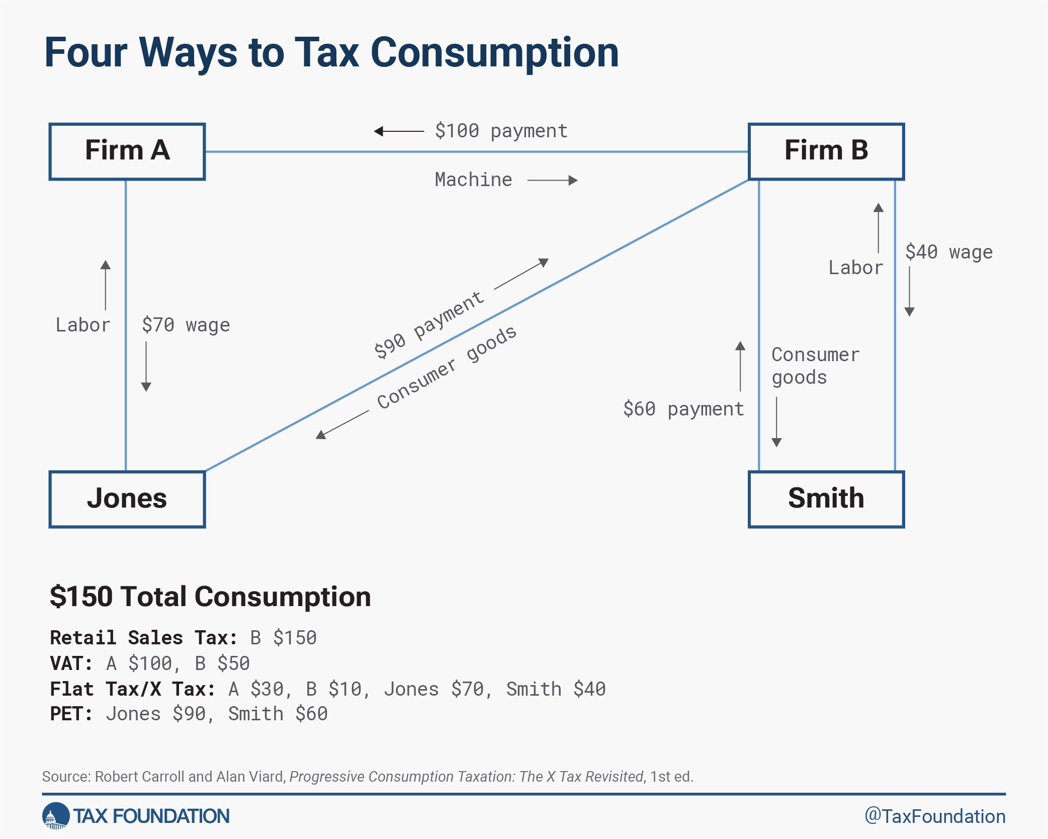
Table 3 outlines four approaches to consumption taxes: the retail sales tax A sales tax is levied on retail sales of goods and services and, ideally, should apply to all final consumption with few exemptions . Many governments exempt goods like groceries; base broadening , such as including groceries, could keep rates lower. A sales tax should exempt business-to-business transactions which, when taxed, cause tax pyramiding . , the value-added tax, the Hall-Rabushka flat tax An income tax is referred to as a “flat tax” when all taxable income is subject to the same tax rate, regardless of income level or assets. or Bradford X Tax, and the consumed-income tax. While each design is different, all four approaches aim to provide neutral tax treatment between saving and consumption.

The retail sales tax is most obviously a tax on consumption, and while the other three approaches may appear less obvious, they too target the same base. Under an ideal retail sales tax, final sales to consumers and government would face a tax, while business to business transactions would not. Retailers would collect and remit the tax revenue to the government. Retail sales taxes are commonly used by U.S. states and municipalities to raise revenue; as of 2023, 45 states and the District of Columbia levy statewide sales taxes. [12]

A VAT is a modified sales tax, collecting the tax incrementally at each stage of the production process. Businesses would pay taxes on their sales less their purchases from other businesses (or alternatively, pay tax on their sales and receive a credit for taxes paid by other businesses). VATs are commonly used across the OECD, and the U.S. is the only country in the OECD with no VAT as of 2023. Consumption taxes made up about 32.1 percent of OECD tax revenue in 2021. [13]

A flat tax is a further modification, splitting the VAT base in two: businesses would pay taxes on their cash flow (sales less purchases, full deductions for capital investment, and compensation paid), while households would pay taxes on compensation received. Applying a progressive rate schedule at the household level, with the top rate matching the rate on business cash flow is known as the X Tax. [14]

Finally, under a consumed income tax, the entire tax would be collected at the household level on income less saving. Income would include wages and compensation, investment income that is spent, and net borrowing, while saving would include increases in bank deposit accounts and purchases of business assets, financial assets, and owner-occupied housing.

As Figure 1 illustrates, though each tax applies to different transactions, each targets the same base: consumption.

Taxing Consumption Rather Than Income Raises Living Standards

Simulations of moving to a consumption tax and econometric studies of policies that incrementally move away from taxing income toward taxing consumption point to the benefits of taxing consumption rather than income in terms of economic growth and increases in welfare.

Ending the income tax penalty on saving and investment by moving to a consumption tax would boost economic output. [15] Depending on how the transition is designed, all income cohorts can enjoy long-run welfare gains. [16] Simulations of replacing individual and corporate income taxes with various types of consumption taxes find increases in long-run economic output of 5 to 9 percent. [17]

For example, a Treasury Department research paper in 2007 found replacing just the U.S. corporate income tax at the time with a business activity tax (a type of consumption tax that does not tax the normal return to saving or investment) would increase the size of the economy from 2.0 percent to 2.5 percent. [18] The paper explained:

First, because a BAT does not tax the normal return to saving or investment, it is likely to stimulate additional saving and investment. Greater investment means businesses would have more capital, which increases workers’ productivity, and ultimately improves living standards. Second, it would likely reduce a variety of tax distortions that arise under the current tax system due to the uneven treatment of investment and other economic activity.

While most simulations focus on how switching to a consumption tax relieves the tax burden on saving, [19] other simulations have looked at the effect on work effort and productivity. For example, a simulation by Carlos E. da Costa and Marcelo R. Santos finds that switching from a progressive income tax to a progressive consumption tax leads to widespread welfare gains because it results in a more efficient allocation of effort and consumption, which enables more efficient revenue generation for redistribution with welfare improvements ranging from 8.6 percent to 19.0 percent. [20]

While a tax reform that reduces the tax burden on higher-income households, such as moving to a consumption tax from a progressive income tax, may increase inequality in the short-term, other, longer-term effects may work to reduce inequality. Further, even if inequality increases, if a tax reform boosts economic growth, absolute living standards can rise across the income spectrum. [21]

As an example, a reduction in income tax progressivity, according to OECD research, “can also raise incentives to save and invest in human capital and so potentially result in increases in lifetime incomes and reductions in lifetime inequality.” [22] The paper continues:

Tax policy should be considered inside a broader framework of structural reforms for inclusive growth. Taxation is often a second-best policy instrument in achieving inclusive growth policy design. In many cases, inclusive growth challenges are best tackled at source… OECD research has highlighted the need to shift the tax mix away from income taxes towards taxes that have less negative impacts on economic growth, including taxes…on consumption.

In other words, prioritizing a tax code that is simple and pro-growth can raise revenues for government spending priorities while boosting living standards relative to the tax system we have today. Like studies that simulate the benefits of moving toward consumption taxes, econometric studies likewise indicate benefits from taxing consumption.

Economist Anh Ngyuen and her coauthors examined the effects of individual income, corporate, and consumption taxes in the United Kingdom from 1973 to 2009. They found that switching from an income tax base The tax base is the total amount of income, property, assets, consumption, transactions, or other economic activity subject to taxation by a tax authority. A narrow tax base is non-neutral and inefficient. A broad tax base reduces tax administration costs and allows more revenue to be raised at lower rates. to a consumption tax base had positive effects on growth, as both individual income and corporate income taxes in their study were found to be more distortionary. [23]

Perhaps the best real-world evidence on the relationship between consumption taxes and economic growth are studies that examine the effects of reducing taxes on saving and capital investment.

For example, the policy of full expensing Full expensing allows businesses to immediately deduct the full cost of certain investments in new or improved technology, equipment, or buildings. It alleviates a bias in the tax code and incentivizes companies to invest more, which, in the long run, raises worker productivity, boosts wages, and creates more jobs. allows businesses to fully deduct the cost of their investments from their taxable income Taxable income is the amount of income subject to tax , after deductions and exemptions . For both individuals and corporations, taxable income differs from—and is less than—gross income. at the time investments occur (a feature of a consumption tax base) rather than depreciating them over time (a feature of an income tax base).

The academic evidence has shown that past reforms in the U.S. that expanded bonus depreciation Bonus depreciation allows firms to deduct a larger portion of certain “short-lived” investments in new or improved technology, equipment, or buildings in the first year. Allowing businesses to write off more investments partially alleviates a bias in the tax code and incentivizes companies to invest more, which, in the long run, raises worker productivity, boosts wages, and creates more jobs. boosted investment and employment. [24] As our colleague noted:

In a study that analyzed how a sample of more than 120,000 firms responded to the two bonus expensing episodes, Zwick and Mahon found that the policy had a substantial impact on investment. Relative to capital assets that were not eligible for bonus expensing, firms increased their investment in eligible equipment by “10.4 percent on average between 2001 and 2004, and 16.9 percent between 2008 and 2010.” In a separate study using the same data set, Garrett, Ohrn, and Suárez Serrato estimated that the two episodes of bonus depreciation Depreciation is a measurement of the “useful life” of a business asset, such as machinery or a factory, to determine the multiyear period over which the cost of that asset can be deducted from taxable income . Instead of allowing businesses to deduct the cost of investments immediately (i.e., full expensing ), depreciation requires deductions to be taken over time, reducing their value and discouraging investment. led to $5.82 trillion of investments and 6.24 million jobs during that period. Depending on the baseline from which the overall budgetary cost is measured, they estimate that the cost-per-job created from the bonus expensing policy was between $20,000 and $50,000.

Moving to full expensing, an incremental step toward a consumption tax base for businesses, reduces the cost of capital and incentivizes businesses to invest more, which in turn boosts productivity growth and economic output, illustrating the benefits of consumption tax reform.

International Examples of VATs

Consumption taxes are a significant source of revenue for governments across the world, making up 32.1 percent of tax revenues on average among OECD countries as of 2021. [25] In most countries, the primary consumption tax is a VAT. The number of countries with a VAT increased from 3 in 1965 to 166 as of 2016. One reason for the growing adoption is the positive efficiency characteristics of the VAT. VATs also replaced turnover taxes that applied to gross receipts, a more inefficient form of tax. [26]

Meanwhile, the United States is the only country in the OECD that does not levy a VAT, instead taxing consumption primarily via retail sales taxes at the state and local level as well as select excise taxes. While the ideal base for sales taxation is all goods and services at the point of sale to the end-user, many retail sales taxes fall on business inputs, hampering economic growth. [27]

The significant and varied experience of OECD countries with VATs can inform the debate of adopting a consumption tax in the U.S. The average standard VAT rate in the OECD is 19.3 percent and the OECD average tax base ratio is 54 percent. [28] Among OECD countries, some stand out as examples for good VAT policies that have relatively low rates, broad tax bases, and low compliance costs. For example, New Zealand has the broadest tax base covering nearly 100 percent of total consumption. Luxembourg and Estonia follow with ratios of 78 percent and 73 percent, respectively.

Several countries, however, exempt or provide special, lower rates to many goods and undermine the efficiency of their VAT or have high administrative burdens. Recent research shows that reduced rates and exemptions are not an effective way of achieving objectives such as supporting low-income households or addressing environmental externalities. [29]

Even if the intention is to support those who earn little income, individuals across the income distribution will also benefit from the reduced rates. Therefore, a refundable food tax credit A tax credit is a provision that reduces a taxpayer’s final tax bill, dollar-for-dollar. A tax credit differs from deductions and exemptions, which reduce taxable income, rather than the taxpayer’s tax bill directly. or other targeted policies would be more effective than the untargeted reduced VAT rates that have proved to be a poor policy tool for addressing income disparities.

Reduced rates and exemptions within VATs can lead to significant reductions in revenue potential as well as higher administrative and compliance costs. For example, in 2020, the average actionable VAT policy gap (additional VAT revenue that could realistically be collected by eliminating reduced rates and certain exemptions) in the EU was 16.4 percent—more than triple the size of the compliance gap. [30]

International experiences with VATs, varied as they may be, all point to the lesson of maintaining as broad a consumption tax base as possible with a single standard rate, and using direct policy means to achieve other goals. Further, specific experiences with VAT implementation can be instructive on other aspects of adopting a consumption tax.

Canada ’s Value-added Tax

The Canadian experience of moving to a VAT illustrates the benefits of reducing the cost of capital for business investment. It also offers important lessons for the administration of a new consumption tax system. Canada illustrates how cooperation between national and subnational governments can reduce administrative costs while warning that carving up the tax base through exemptions and rebates claws back some benefits of moving to a broad-based consumption tax.

Canada levies a federal value-added tax (called the Goods and Services Tax, or GST) at a rate of 5 percent. The GST in Canada replaced an earlier tax called the Manufacturer’s Sales Tax (MST). Nearly half the revenue collected from the MST came from business inputs rather than final consumption, leading to a higher cost of capital for business investment as the tax cascaded through the steps of the production process and increased final prices to consumers. [31] One of the leading factors for VAT reform was to remove the disincentive for business investment created by taxing business inputs under the MST.

After initial implementation of the VAT, through decades of negotiations between federal and provincial governments, five provinces now levy fully harmonized provincial VATS (called Harmonized Sales Taxes or HSTs) and Quebec levies the Quebec Sales Tax (QST, a VAT). [32] The GST and HST are now jointly administered and do not require businesses to complete separate filings because they apply to the same tax base and follow the same tax rules. The QST is structured the same way as the GST and HST, but it is administered separately by Revenue Quebec (which also administers the GST in the province). Additionally, some provinces levy a completely separate retail sales tax that is not a VAT.

Research conducted in the period after several provinces replaced their retail sales taxes with harmonized VATs found investment in machinery and equipment rose 12.2 percent above trend in the years following the reforms, resulting from a reduction in the tax burden on business capital. [33]

Of particular interest to U.S. policymakers, as detailed by Richard M. Bird of the University of Toronto, the fiscal reform in Canada that led to the GST “has not resulted to any significant extent either in higher taxes or bigger governments, but rather in governments being able to finance their expenditures in economically less damaging ways.” [34] The value-added taxes in Canada, unique from VATs in Europe, are listed separately on receipts to final consumers. The heightened salience of the VATs may help create political pressure to keep rates from rising.

Bird also notes that while administration of the tax is considered good compared to other countries, the administrative problems that are encountered are most prominently due to tax design rather than management. In particular, decisions to narrow the base and provide complex rebates increase the administrative costs of the tax, offering another lesson to U.S. policymakers of the importance of a broad, simple tax base.

Australia ’s Value-added Tax

The Australian experience demonstrates the short-lived impact on prices, consumer spending, retail sales, and the overall economy when transitioning to a consumption tax.

In July 2000, Australia cut personal income taxes and abolished several harmful excise and sales taxes and replaced them with a 10 percent Goods and Services Tax (GST, another name for a VAT). The reform included bonus payments to retirees, increases in pensions, child tax offsets and family benefit increases, and payments to individuals outside the tax and pension systems, in part to relieve the transitional impact of the GST on particular groups.

Government studies indicate the effect of implementing the GST on prices was a one-off and transitory increase in the price level, and other transitional impacts “appear to have ‘washed out’ over the first two years.” [35] Independent research likewise found a clear inflationary impact in the quarter the tax was implemented but no additional price effects before or after that single quarter. [36]

The Australian government also analyzed the transition to a consumption tax in Japan , New Zealand, Canada, and Singapore, finding a general pattern of acceleration in household consumption prior to adoption, followed by a decline, and a distinct, one-off increase in the price level. [37] Their experiences suggest price level changes should not be a major concern for U.S. policymakers interested in moving toward consumption taxes.

Flat Taxes in Estonia, Latvia , and Slovakia

Starting in the 1990s, several former Soviet-bloc countries abandoned their progressive income tax systems and replaced them with flat taxes. Although they still taxed income broadly, some sought to eliminate the prevalence of double taxation by eliminating taxes on dividends and inheritances, moving closer to a consumption tax system.

Estonia was the first to adopt a flat tax, imposing a 26 percent flat rate in 1994, which has since been lowered to 20 percent. [38] In the early 2000s, Estonia reformed its corporate tax system to tax profits only when they are distributed at 20 percent, fully exempting dividends from individual income taxation. [39] Estonia also imposes a VAT of 20 percent.

Following Estonia’s lead, Latvia also switched to a flat tax system in the 1990s, adopting a rate of 25 percent which has since fallen to 23 percent, while also imposing a VAT at a slightly lower rate. Latvia and Georgia are the only other countries to tax distributed profits only. Latvia levies the tax at a 20 percent rate like Estonia, and Georgia levies it at a 15 percent rate. [40]

Slovakia pursued similar reform in the early 2000s. Prior to 2004, Slovakia imposed a progressive tax A progressive tax is one where the average tax burden increases with income. High-income families pay a disproportionate share of the tax burden, while low- and middle-income taxpayers shoulder a relatively small tax burden. on income, a corporate income tax, and a VAT. Following a desire to create a simple and transparent tax system, Slovakia switched to a flat tax of 19 percent on all income and eliminated all taxes on dividends and inheritances. [41] The reform effectively removed the double taxation of income that characterizes most income tax systems. The policies were eventually reversed in 2012 under a different administration and a progressive income tax was reinstated. One OECD analysis estimated that a reversal of the flat tax in Slovakia would reduce aggregate incomes, and the reduction in economic growth would reduce tax revenue. [42]

Each country experienced substantial growth post-reform, with Estonia and Latvia converging significantly with other European countries in terms of GDP per capita. [43] Slovakia also experienced strong growth in the 2000s, with foreign direct investment (FDI) in particular showing substantial increases. [44] One paper estimated that switching to a distributed profits tax A distributed profits tax is a business-level tax levied on companies when they distribute profits to shareholders, including through dividends and net share repurchases (stock buybacks). in Estonia boosted firm investment and labor productivity, and also reduced firms reliance on debt-financing. [45] Follow-up modeling found similar positive effects for the Estonian reform. [46]

Practical and Implementation Issues in the U.S.

The current u.s. hybrid tax system and its effects.

The current federal tax code is not a pure version of either a consumption tax or income tax. It most closely resembles a broad income tax, generally taxing a person’s current earnings (whether spent or saved) plus the change in the value of their existing assets (such as dividends, capital gains, interest, etc.). In some cases, however, it adopts consumption tax provisions like retirement savings accounts for individuals and investment deductions for businesses. [47] In all, the current U.S. tax system distorts saving and investment decisions and holds back economic growth, reducing the living standards of American families.

For example, the current business tax system reduces incentives to invest by its differing treatment of different types of investment, firm structure (corporate versus noncorporate), and financing method. The nearby table illustrates the distortions created under current law as different types of investments face drastically different marginal tax rates in 2023.

Higher marginal tax rates on capital increase the required rate of return for a given investment to be viable, meaning the tax system can prevent otherwise worthwhile investments from occurring. Over time, high marginal tax rates can reduce the size of the capital stock, which harms workers by reducing labor productivity and wages. [48]

Standard economic analysis assigns 25 percent to 50 percent of the corporate income tax burden to workers, and in some cases, workers’ share of the burden can be even higher. [49] Further, research in Germany has shown that higher corporate taxes reduce wages the most for low-skilled, women, and young workers, which significantly reduces the assumed progressivity of corporate income taxes. [50]

In addition to discouraging decisions to work, save, and invest, complying with existing income tax rules is very costly. Tax Foundation estimates the compliance burden across individual and business income tax returns exceeds $300 billion annually. [51] Each year, billions of hours and dollars are diverted away from productive uses, instead wasted on complying with an increasingly complex web of tax rules.

Compliance costs are particularly important for entrepreneurs and their decision to enter or exit an industry. High compliance costs can discourage entrepreneurs from beginning a venture, creating structural barriers to entry beyond the negative economic incentives created by high marginal tax rates on work, saving, and investment. [52] This, in turn, reduces living standards for families with children, both for families who are entrepreneurs themselves and for families who benefit from increased entrepreneurship.

Social Benefits Embedded in the Tax System Lead to Complexity

Consumption tax reform can boost after-tax income for families with children, simplify the tax filing experience, and ensure a robust system for raising revenue for government programs.

The individual income tax system contains some of the U.S.’s largest support programs for families with children, most notably the Child Tax Credit (CTC) and the Earned Income Tax Credit (EITC), which encourage work participation and supplement income. Both credits phase in with earned income (wages or self-employment income) to create an incentive to work, plateau, and then phase-out when income exceeds certain thresholds. In 2022, the EITC provided $63 billion in support; the CTC, $124 billion. [53] Both credits are also refundable, meaning the credits allow a taxpayer to reduce their income tax liability until it reaches zero and then receive any additional credit they are eligible for as a refund payment.

The Congressional Research Service (CRS) estimates the income tax reduces the share of total individuals in poverty by 15 percent (from 14.7 percent to 12.5 percent in 2020, concentrated among families with both children and workers). [54] Together, the refundable CTC and EITC lifted more than 5 million people above the poverty line in 2020. [55] More recently, the temporary expansion of the CTC during the pandemic under the American Rescue Plan Act, which increased the maximum credit and made it fully available to households with little to no income, lifted an additional estimated 2.1 million children above the poverty line. [56]

Reducing material hardship is a worthy goal. Income poverty causes negative outcomes for children; and many studies have found that reducing material poverty, including through income transfers, translates into improved outcomes for children. [57]

For instance, a review of the EITC literature by the National Academy of Sciences concluded, “Periodic increases in the generosity of the Earned Income Tax Credit Program have improved children’s educational and health outcomes” such as reducing the likelihood of low infant birth weight and increasing college attendance. [58]

Embedding much of the social safety net in the income tax code, however, creates complexities for families and limits the effectiveness in providing support to households who do not file taxes.

The CTC and EITC depend on often-complicated family characteristics, leading to difficulties for families. For example, to qualify for the EITC, taxpayers must meet at least 20 requirements. [59] Partially as a result, the EITC suffers from a relatively high rate of incorrectly issued payments—it reached 32 percent, or $18 billion, in fiscal year 2022. [60] Both overpayments and underpayments are mostly due to qualifying child errors. [61]

The relationship, residency, and identification tests legally required to qualify for the CTC are likewise difficult for families to comply with and for the IRS to enforce, especially for families with complex living arrangements. [62] It suffered from an overpayment rate of 16 percent or $5 billion in fiscal year 2022. [63] For several years, the Taxpayer Advocate’s Annual Report to Congress has recommended reform of the credits chiefly because of their complexity. [64]

Perhaps a reflection of the high improper payment rate, audit A tax audit is when the Internal Revenue Service ( IRS ) conducts a formal investigation of financial information to verify an individual or corporation has accurately reported and paid their taxes. Selection can be at random, or due to unusual deductions or income reported on a tax return. rates for EITC returns are disproportionately high, creating another significant burden for lower-income families.

In 2017, more than 27 million tax returns claimed the EITC while about 126 million did not. The IRS audited 1 percent of the EITC returns, resulting in 280,000 audits, and audited 0.3 percent of non-EITC returns, resulting in 420,000 audits. [65] Research finds lower-income taxpayers often face barriers to understanding and effectively participating in audits, further increasing the disproportionate burden. [66]

Embedding support in the tax system creates additional difficulties for low-income families. Unlike other relief programs that provide monthly payments, the refundable tax credits are lump sum payments. Research indicates the credits supply about 9 to 13 percent of income for lower-income households, [67] meaning some families receive the largest single share of their annual income at tax filing time.

It can, however, be difficult to predict the size of credits from year to year. For example, about 40 percent of low-income families with children see EITC decreases of more than $500, while 19 percent see CTC decreases of more than $500. [68] The decreases are most often due to higher incomes, but unpredictable changes in family characteristics can also cause changes. Large, yearly swings in eligible credit size present a challenge for advancing the benefits on a regular basis outside the tax filing season. Further, most refundable tax credit A refundable tax credit can be used to generate a federal tax refund larger than the amount of tax paid throughout the year. In other words, a refundable tax credit creates the possibility of a negative federal tax liability. An example of a refundable tax credit is the Earned Income Tax Credit ( EITC ). beneficiaries rely on paid tax preparers whose fees can capture up to 20 percent of EITC refunds. [69]

While the current income tax code reduces material hardship, primarily for working taxpayers with children, it falls short on simplicity and efficiency grounds. The status quo warrants massive simplification.

Distributional and Design Choices

Two commonly cited concerns when moving to a consumption tax are the distributional impact and transition. We briefly discuss both concerns and highlight options policymakers may implement to address them.

Consumption taxes are generally assumed to have a regressive distribution. When the burden of a consumption tax is measured as a share of current income, studies tend to show lower-income people pay a higher share of their income than higher-income people. That is primarily because lower-income households tend to consume a relatively larger share of their income than higher-income households, while higher-income households save a larger share of their income.

When consumption taxes are measured as a share of current expenditures, however, research indicates they are proportional, or in some cases, even progressive. [70] The expenditures approach is useful because it recognizes that income saved will eventually be spent, facing the consumption tax at that time.

Nevertheless, measured as a share of current income, moving to a consumption tax would likely be less progressive than the income tax system we have today. As such, when designing a consumption tax, policymakers will likely consider elements to offset that distributional effect. The most efficient way to increase the progressivity of a consumption tax while also maintaining a broad tax base and single tax rate would be to offer targeted relief to lower-and middle-income households.

Replacing the current income tax system with a consumption tax would create transitional effects for people currently holding capital by affecting asset values. On the one hand, repealing the income tax would increase the after-tax return to capital, increase demand for capital, and thus increase its value. On the other hand, imposing a consumption tax would reduce the value of existing capital. The net impact depends on various factors. It is likely the value of most existing capital falls at least somewhat, meaning shareholders face a one-time tax burden on their wealth (their existing saving) at the time of transition. The one-time tax on existing wealth would be progressive given that asset ownership is skewed toward the wealthy.

Moving to a consumption tax also requires deciding whether to apply the tax on an origin basis, as today’s income taxes are, or on a destination basis, as VATs are. Destination-based taxes mean only activity within a country’s borders faces the tax; that treatment is achieved by applying the tax to imports and exempting exports. [71] The decision of how to apply the tax at the border on an origin or destination basis results in equal treatment and has no effect on international competitiveness, but it can have transitional effects. [72]

Other considerations involve how to treat fringe benefits. The current income tax allows employers to deduct what they spend on health insurance and other fringe benefits and does not tax such items as income for individuals. Under a flat tax, employers would still deduct all forms of compensation, including fringe benefits, and households would pay taxes on all forms of compensation they receive.

Alternatively, fringe benefits could be taxed at the source, meaning firms would not deduct the cost of fringe benefits and households would not pay tax on fringe benefits, and could be subject to payroll taxes.

Offering some form of relief to mitigate transition effects is likely warranted, though it should be simple and well-targeted. Any revenues used for transition relief require a higher tax rate to reach revenue neutrality, thus reducing economic efficiency. [73]

Finally, questions of administration, particularly with respect to state sales tax systems and state conformity with the federal income tax code, would need to be addressed. Enticing states to conform to a federal consumption tax could lead to additional economic, administrative, and compliance cost reductions.

Modeling Consumption Tax Reforms for the United States

Economic, revenue, and distributional effects of a value-added tax and rebate.

The first consumption tax reform we model implements a value-added tax and rebate to replace the corporate income tax and child tax credit, earned income tax credit, and child and dependent care tax credit. [74]

The value-added tax base is broadly defined to include all consumption. It is defined as labor income (wages and salaries as well as other forms of labor compensation), capital income across all sectors (less investment, which is deductible under a VAT), and net imports (see Appendix Table 1 in Modeling Notes). [75] The broad VAT base is equal to about 72 percent of GDP based on 2021 levels.

Under the broad VAT base, we modeled a rate of 6.4 percent and rebate of $525 per filer and $2,100 per dependent starting in 2024 and adjusting for inflation Inflation is when the general price of goods and services increases across the economy, reducing the purchasing power of a currency and the value of certain assets. The same paycheck covers less goods, services, and bills. It is sometimes referred to as a “ hidden tax ,” as it leaves taxpayers less well-off due to higher costs and “bracket creep,” while increasing the government’s spending power. annually thereafter. Overall, the option increases the long-run size of the economy by 0.3 percent and the capital stock by 1.9 percent. Wages would rise by 1.2 percent while hours worked would fall by 531,000 full-time equivalent jobs.

Replacing the corporate income tax with a value-added tax lowers the cost of capital, which leads to a larger capital stock and higher wages as productivity grows. While a value-added tax does not discourage business investment or household saving, it does still distort labor supply decisions. It creates a wedge between the amount of money a person earns from labor and how much consumption a person can afford after tax, which leads to a reduction in hours worked. That is why the reform reduces hours worked, even as it results in higher economic output, investment, and wages through its reduction in the cost of capital.

Eliminating individual tax credits that phase-in and phase-out with income leads to opposing effects on marginal income tax rates that, on net, reduce marginal tax rates overall and lead to a slightly positive economic effect. Replacing the credits with a flat, lump sum credit offsets some loss of benefit without distorting marginal income tax rates and significantly simplifies the credits. The lump sum credit is worth $525 per filer and $2,100 per dependent.

Families at different income levels would experience different changes in their net benefits under the proposed reforms. For example, under current law, a single parent with $5,000 in income and one child dependent would qualify for nearly $2,100 of tax credits. The same family would qualify for $2,625 under the proposed reform, without facing the complexities of the current tax credit system. Families with no incomes would newly qualify for full benefits under the reform, whereas currently they receive none.

The EITC currently reaches a maximum credit of $3,995 for families with one dependent or $7,430 for three or more dependents. Families higher on the EITC and CTC phase in ranges could see a decrease in their net benefits. For example, a family of joint filers earning $35,000 with two child dependents would qualify for about $7,000 to $9,000 of tax credits currently, which would fall to $5,250 under the proposed reform. [76]

Over the 10-year budget window, the option raises revenue by $569 billion on a conventional basis and by $24 billion on a dynamic basis after accounting for economic effects. The reform raises less revenue on a dynamic basis because initially the economic effect of the reform is negative: labor supply responds relatively fast to the introduction of a value-added tax, while investment responds relatively slow to the removal of the corporate income tax.

In the long run, the plan has a positive economic effect and is approximately revenue neutral on a conventional basis.

In the long run, as measured on a conventional basis, after-tax income of all taxpayers increases slightly on average, as the plan is roughly revenue neutral. The bottom 20 percent of taxpayers would see an increase in after-tax income of 5.5 percent. On a dynamic basis, after-tax income increases by 0.3 percent on average, when factoring in the positive economic effects of the reform.

Looking at families with children, we estimate that on a conventional basis, after-tax income increases by 4.0 percent for the bottom 20 percent of income earners and by 2.1 percent on average overall.

Economic, Revenue, and Distributional Effects of a Tax on Business Profits and Household Compensation

The second option modifies the first by splitting the broad value-added tax into two components: a tax at the business level on cash flow profits and a progressive tax at the household level on compensation with a per person credit. The business profits and household compensation tax replace the current corporate and individual income taxes and the per person credit replaces the EITC, CTC, and CDCTC.

The base of the tax is equal to a broad-based VAT. For businesses, it would provide full and immediate expensing for all business investment, flip the treatment of interest so that it is not deductible and not taxable, remove foreign income from the tax base, remove general business tax credits, and be border adjusted. The resulting measure of profit would face a flat 30 percent tax.

Households would pay taxes on wages and salaries as well as supplements such as employer-provided health insurance and other fringe benefits but would not pay taxes on capital income such as capital gains, interest, or dividends. Compensation would be taxed progressively as described in Table 9 below, with rates ranging from 10 percent to 30 percent. All itemized deductions and the CTC, EITC, and CDCTC would be eliminated. A lump sum credit of $600 per filer and $2,400 per dependent would replace the eliminated credits.

Replacing the corporate and non-corporate income taxes with a cash flow tax that allows full expensing of all capital investment significantly reduces the cost of capital and thus incentivizes new domestic investment.

Restructuring the individual income tax to fall on only labor income, instead of labor income and the returns to saving and investment, boosts incentives to save and work, as does eliminating the net investment income tax (a surtax A surtax is an additional tax levied on top of an already existing business or individual tax and can have a flat or progressive rate structure. Surtaxes are typically enacted to fund a specific program or initiative, whereas revenue from broader-based taxes, like the individual income tax , typically cover a multitude of programs and services. on certain investment income under current law). Broadening the base to eliminate itemized deductions and tax non-wage compensation such as health insurance and fringe benefits increases the tax burden on labor but reduces distortions in the current tax base and offsets the costs of the other reforms.

The combined effect of better structured tax bases is to boost incentives to work, save, and invest. Additionally, setting the top tax rate on household income at 30 percent to match the tax rate on business profits reduces incentives to recharacterize income at the margin, which reduces administrative and compliance costs too.

Eliminating individual tax credits that phase-in and phase-out with income leads to opposing effects on marginal income tax rates that, on net, reduce marginal tax rates overall and lead to a slightly positive economic effect. Replacing the credits with a flat, lump sum credit offsets some loss of benefit without distorting marginal income tax rates and simplifies rules leading to easier administration and compliance.

Using the same examples as above, a single parent with $5,000 in income and one child dependent would qualify for nearly $2,100 of tax credits under current law. The same family would qualify for $3,000 under the proposed reform. A family of joint filers earning $35,000 with two child dependents would qualify for about $7,000 to $9,000 of tax credits currently, which would fall to $6,000 under the proposed reform.

Overall, the business profits and household compensation tax would boost long-run GDP by 1.9 percent, expand the capital stock by 2.8 percent, lift wages by 1.2 percent, and increase hours worked by 886,000 full-time equivalent jobs.

Within the 10-year budget window, the reform would reduce federal revenue by slightly more than $1 trillion on a conventional basis. When factoring in the positive economic feedback from increased investment and work, federal revenue would decrease by about $130 billion.

In the long-run, the plan is roughly revenue neutral on a conventional basis.

On a long-run conventional basis, taxpayers overall would see a slight change in after-tax income, as the reform is nearly revenue neutral. Taxpayers in the bottom quintile, however, would see a 5.8 percent increase in after-tax income, largely a function of replacing complex, refundable tax credits with simple, lump sum tax credits. The increase would be much smaller for the second quintile overall, while taxpayers from the 40th to 99th percentiles would, on average, see a reduction in after-tax income. Taxpayers in the top 1 percent would see an increase in after-tax income of 7.9 percent.

On a dynamic basis, after-tax income of taxpayers overall would rise by 1.8 percent due to increased economic growth and higher incomes. The bottom three quintiles would see higher after-tax income as a result of the positive economic impact of the reform. Taxpayers in the fourth quintile would still see a slight decrease in after-tax income, as would taxpayers in the 80th to 99th percentile.

For taxpayers with child dependents, after-tax income on a long-run conventional basis would increase by 4.2 percent for the bottom 20 percent of families with children. The simplified lump sum credits are especially impactful for taxpayers with children, increasing income by more than the overall average for the bottom 60 percent of taxpayers.

Improvements in the long-run standard of living largely depend on peoples’ willingness to work and to invest in capital. Tax policy has a significant effect on decisions to work and to invest by changing the after-tax benefits of both.

While increased economic growth and material living standards do not make up the entirety of human well-being, material prosperity is strongly correlated with better outcomes for people across a variety of alternate measures.

Reforming the current income tax system toward a consumption tax system would support rising living standards and economic growth. Combined with a simpler system of providing tax credits for individuals and children, such a reform could reduce the economic, administrative, and compliance costs imposed by the current tax system.

Appendix: Modeling Notes

We use the Tax Foundation General Equilibrium Tax Model to estimate the impact of tax policy changes in terms of economic, budgetary (tax revenue), and distributional effects. Economic impact measures include GDP, wages, employment, capital stock, investment, consumption, saving, and the trade deficit. Conventional tax revenue estimates hold the size of the economy constant but include certain behavioral effects of tax policy, such as profit shifting Profit shifting is when multinational companies reduce their tax burden by moving the location of their profits from high-tax countries to low-tax jurisdictions and tax havens. . Dynamic revenue estimates consider both behavioral and macroeconomic effects of tax policy on revenue. Our revenue and distributional estimates do not include the impact of the proposed tax changes on non-filers.

Appendix Tables 1 and 2 illustrate the construction of the value-added tax base using data from the Bureau of Economic Analysis for calendar year 2021. The broad-based VAT illustrates the tax base in the Tax Foundation’s General Equilibrium model and includes an adjustment for housing so that owner-occupied homes are taxed on a pre-pay basis.

Simply multiplying the VAT rate by the proper economic accounts would overstate the potential revenue impact of a VAT because any tax will suffer from some tax avoidance. As such, we reduce the VAT base to account for potential tax avoidance. We assume that the VAT noncompliance rate would be 15 percent.

If lawmakers excluded certain categories of goods or services from the VAT base, it would require a higher tax rate to generate the same revenue as the option we simulated. Appendix Table 2 illustrates one such example of a narrow tax base.

Under the household compensation tax, to model the tax revenue and distributional effects associated with eliminating the exclusion for employer-sponsored health insurance (HI) and other fringe benefits, we used the tax expenditure Tax expenditures are a departure from the “normal” tax code that lower the tax burden of individuals or businesses, through an exemption , deduction , credit , or preferential rate. Expenditures can result in significant revenue losses to the government and include provisions such as the earned income tax credit ( EITC ), child tax credit ( CTC ), deduction for employer health-care contributions, and tax-advantaged savings plans. estimates provided by the Treasury Department, the HI benefit amounts provided by the Bureau of Economic Analysis, and the distributional analysis provided by the Congressional Budget Office.

We then estimated the HI benefit as a share of wages and added it as an additional source of income in our modeling of the household compensation tax, also including it in our economic and distributional analysis. We assume that under the reform, firms shift compensation away from HI and other fringe benefits towards cash compensation, such that in the 10th year all compensation is in cash. The extent to which the shift to cash compensation occurs is uncertain, however, and if the shift is only partial, it would raise less revenue than what our analysis assumes.

[1] Charles W. Cobb and Paul H. Douglas, “A Theory of Production,” The American Economic Review 18, no. 1, (March 1928): 139-165, https://www.aeaweb.org/aer/top20/18.1.139-165.pdf .

[2] Congressional Budget Office, “How Labor Supply Responds to Changes in Fiscal Policy,” October 2012, https://www.cbo.gov/sites/default/files/cbofiles/attachments/10-25-2012-Labor_Supply_and_Fiscal_Policy.pdf .

[3] Giorgia Maffini, Jing Xing, and Michael P Devereux, “The impact of investment incentives: evidence from UK corporation tax returns,” Working Papers 1601, Oxford University Centre for Business Taxation, 2016, https://ideas.repec.org/p/btx/wpaper/1601.html .

[4] Organization for Economic Cooperation and Development, “Measuring Well-bring and Progress: Well-being Research,” https://www.oecd.org/wise/measuring-well-being-and-progress.htm .

[5] Robert Wood Johnson Foundation, “Well-Being: Expanding the Definition of Progress,” May 2020, https://www.rwjf.org/en/insights/our-research/2020/05/well-being–expanding-the-definition-of-progress.html .

[6] J.F. Helliwell et al., “Self-reported life satisfaction vs. GDP per capita, 2022,” Our World in Data, Mar. 3, 2023, https://ourworldindata.org/grapher/gdp-vs-happiness .

[7] R. Fouquest, “Air pollution vs. GDP per capita, 1700 to 2015,” Our World in Data, Feb. 15, 2016 https://ourworldindata.org/grapher/air-pollution-vs-gdp-per-capita ; “There is a very strong positive relationship [between trust and GDP per capita]. Most academic studies find that this relationship remains after controlling for further characteristics. And similar results can also be obtained by looking at other measures of economic outcomes.” For more, see Esteban Ortiz-Ospina and Max Roser, “Trust,” Our World in Data, 2016, https://ourworldindata.org/trust .

[8] Max Roser, Estaban Ortiz-Ospina, and Hannah Ritchie, “Life expectancy and GDP,” Our World in Data, October 2019, https://ourworldindata.org/life-expectancy#life-expectancy-and-gdp . See also Max Roser, Hannah Ritchie and Bernadeta Dadonaite, “Child and Infant Mortality,” Our World in Data, November 2019, https://ourworldindata.org/child-mortality#child-mortality-and-income-level .

[9] Karen Dynam and Louise Sheiner, “GDP as a Measure of Economic Well-being,” Brookings Institution Hutchins Center on FIscal & Monetary Policy, August 2018, https://www.brookings.edu/wp-content/uploads/2018/08/WP43-8.23.18.pdf .

[10] See, for example, Randall K.Q. Akee et al., “Parents’ Income and Children’s Outcomes: A Quasi-Experiment,” American Economic Journal: Applied Economics , 2, no. 1 (Jan. 2010), https://www.aeaweb.org/articles?id=10.1257/app.2.1.86 , and Kerris Cooper and Kitty Stewart, “Does Household Income Affect Children’s Outcomes? A Systematic Review of the Evidence,” Child Indicators Research , November 4, 2020, https://link.springer.com/article/10.1007/s12187-020-09782-0 .

[11] Anthony Atkinson and Joseph Stiglitz, “The design of tax structure: Direct versus indirect taxation,” Journal of Public Economics 6 (1976): 55-75; Louis Kaplow, “On the undesirability of commodity taxation even when income taxation is not optimal,” Journal of Public Economics 90 (2006): 1235-1250; Joseph Bankman and David Weisbach, “The Superiority of an Ideal Consumption Tax over an Ideal Income Tax,” Stanford Law Review 58 (2005): 1413-1456.

[12] Janelle Fritts, “State and Local Sales Tax Rates, 2023,” Tax Foundation, Feb. 7, 2023, https://taxfoundation.org/data/all/state/2023-sales-taxes/ .

[13] Daniel Bunn and Cecilia Perez Weigel, “Sources of Government Revenue in the OECD, 2023,” Tax Foundation, Feb. 23, 2023, https://taxfoundation.org/data/all/global/oecd-tax-revenue-by-country-2023/ .

[14] See Robert Carroll and Alan Viard, Progressive Consumption Taxation: The X Tax Revisited , 1st ed. ( Washington , D.C.: The AEI Press, 2012), 68-81 for more discussion on why the top household compensation tax rate should match the business cash-flow rate to prevent income mischaracterization at the margin.

[15] Ibid 6-11.

[16] David Altig, et al., “Simulating Fundamental Tax Reform in the U.S.” The American Economic Review , (June 2001), https://eml.berkeley.edu/~auerbach/ftp/taxreform/flatfinal.pdf .

[18] Office of Tax Policy U.S. Department of the Treasury, “Approaches to Improve the Competitiveness of the U.S. Business Tax System for the 21st Century,” Dec. 20, 2007, https://home.treasury.gov/system/files/131/Report-Improve-Competitiveness-2007.pdf .

[19] A consumption tax still falls on returns to capital arising from risk taking, entrepreneurial or market power, and luck. Such returns typically accrue to higher income and higher wealth households, meaning a share of their returns to capital still face tax. As such, the idea that “consumption tax reform is a sop to the rich is almost certainly unfair, especially if a progressive consumption tax,” is considered. See R. Glenn Hubbard, “Would a Consumption Tax Favor the Rich?” in Kevin A. Hassett and Alan J. Auerbach, Toward Fundamental Tax Reform , https://www.aei.org/wp-content/uploads/2013/12/-toward-fundamental-tax-reform-chapter-5_130947205941.pdf .

[20] Carlos E. da Costa and Marcelo R. Santos, “Progressive Consumption Taxes,” Jan. 12, 2021, https://papers.ssrn.com/sol3/papers.cfm?abstract_id=3803684 .

[21] Oguzhan Akgun, Boris Cournède, and Jean-Marc Fournier, “The effects of the tax mix on inequality and growth,” OECD Economics Department Working Papers, No. 1447, Dec. 15, 2017, https://doi.org/10.1787/c57eaa14-en .

[22] Pierce O’Reilly, “Tax policies for inclusive growth in a changing world”, OECD Taxation Working Papers, No. 40, Dec. 18, 2018, https://doi.org/10.1787/1fdafe21-en .

[23] Anh Ngyuen, Luisanna Onis, and Raffaele Rossi, “The Macroeconomic Effects of Income and Consumption Tax Changes,” American Economic Journal , Vol. 13, No.2 (May 2021): 439-66, https://www.aeaweb.org/articles?id=10.1257/pol.20170241 ; Countries may have economic, social, and cultural differences that limit applicability to the U.S. External validation may always be tentative and it is important to use carefully designed empirical research when making cross-country comparisons.

[24] Scott Hodge, “Empirical Evidence Shows That Expensing Leads to More Investment and Higher Employment,” Tax Foundation, May 19, 2020, https://taxfoundation.org/expensing-leads-to-more-investment-and-higher-employment/ .

[25] Daniel Bunn and Cecilia Perez Weigel, “Sources of Government Revenue in the OECD, 2023,” Tax Foundation, Feb. 23, 2023, https://taxfoundation.org/oecd-tax-revenue-by-country-2023/ . .

[26] O’Reilly, “Tax policies for inclusive growth in a changing world”; Garrett Watson and Daniel Bunn, “Learning from Europe and America’s Shared Gross Receipts Tax A gross receipts tax, also known as a turnover tax, is applied to a company’s gross sales, without deductions for a firm’s business expenses, like costs of goods sold and compensation. Unlike a sales tax , a gross receipts tax is assessed on businesses and apply to business-to-business transactions in addition to final consumer purchases, leading to tax pyramiding . Experience,” Feb. 12, 2019, Tax Foundation, https://taxfoundation.org/blog/europe-america-gross-receipts-taxes/ .

[27] Janelle Fritts and Jared Walczak, “2022 State Business Tax Climate Index,” Tax Foundation, Dec. 16, 2021, https://taxfoundation.org/research/all/state/2022-state-business-tax-climate-index/ .

[28] Daniel Bunn, Cristina Enache, and Ulrik Boesen, “Consumption Tax Policies in OECD Countries,” Tax Foundation, Jan. 26, 2021, https://taxfoundation.org/data/all/global/consumption-tax-policies/ : Daniel Bunn and Lisa Hogreve, International Tax Competitiveness Index 2022 , Tax Foundation, Oct. 17, 2022, https://taxfoundation.org/research/all/global/2022-international-tax-competitiveness-index/ .

[29] Rita de la Feria and Michael Walpole, “The Impact of Public Perceptions on General Consumption Taxes,” British Tax Review 67, no. 5 (Dec. 4, 2020), 637-669, https://papers.ssrn.com/sol3/papers.cfm?abstract_id=3723750 .

[30] Cristina Enache, “VAT Expansion and Labor Tax Cuts,” Tax Foundation, Jan. 10, 2023, https://taxfoundation.org/vat-tax-expansion-and-labor-tax-cuts/ .

[31] Richard M. Bird, “The GST/HST: Creating an Integrated Sales Tax in a Federal Country,” The School of Public Policy Publications (SPPP) ; Calgary Vol. 5, (2012), https://www.proquest.com/docview/2204835860 .

[32] PwC Worldwide Tax Summaries, “Canada Corporate – Other taxes,” June 15, 2023, https://taxsummaries.pwc.com/canada/corporate/other-taxes .

[33] Michael Smart and Richard Miller Bird, “The Impact on Investment of Replacing a Retail Sales Tax by a Value-Added Tax: Evidence from Canadian Experience,” Institute for International Business , No. 15, (June 2008), https://ssrn.com/abstract=1273773 .

[35] Australia Treasury, “Preliminary assessment of the impact of The New Tax System,” April 3, 2003, https://treasury.gov.au/publication/economic-roundup-autumn-2003/preliminary-assessment-of-the-impact-of-the-new-tax-system .

[36] Abbas Valadkhani and A. P. Layton, “Quantifying the Effect of GST on Inflation in Australia’s Capital Cities: An Intervention Analysis,” Australian Economic Review, 37, no. 2, (March 2004), https://ro.uow.edu.au/cgi/viewcontent.cgi?article=1410&context=commpapers .

[37] Australia Treasury, “Preliminary assessment of the impact of The New Tax System.”

[38] Daniel J. Mitchell, “Flat Tax is the Way of the Future.” Heritage Foundation, March 2006, https://www.heritage.org/taxes/commentary/flat-tax-the-way-the-future .

[39] William McBride, Garrett Watson, and Erica York. “Taxing Distributed Profits Make Taxation Simple and Efficient,” Tax Foundation, Mar. 1, 2023, https://taxfoundation.org/distributed-profits-tax-us-businesses/ .

[40] Amir El-Sibaie, “Latvia Joins the Cash Flow Tax Club,” Tax Foundation, Apr. 16, 2018. https://taxfoundation.org/latvia-cash-flow-tax/ .

[41] Scott Hodge. “Flat Tax Lessons from Slovakia,” Tax Foundation, Oct. 26, 2011, https://taxfoundation.org/flat-tax-lessons-slovakia .

[42] Michal Horvath et al., “The End of the Flat Tax Experiment in Slovakia…” Economic Modeling , Vol. 80, (August 2019): 171-184, https://www.sciencedirect.com/science/article/abs/pii/S0264999317316425 .

[43] European Central Bank, “Convergence and Adjustment in the Baltic States,” 2017, https://www.ecb.europa.eu/pub/pdf/other/ebbox201705_01.en.pdf .

[44] Tomasz Daborowski. “Slovakia’s Economic Success and the Global Crisis,” Centre for Eastern Studies, 2009, https://www.files.ethz.ch/isn/96500/commentary_19.pdf .

[45] Jaan Masso, Jaanika Merikull, and Pritt Vahter, “Gross Profit Taxation Versus Distributed Profit Taxation and Firm Performance: Effects of Estonia’s Corporate Tax Reform,” The University of Tartu Faculty of Economics and Business Administration, Working Paper No. 81, March 23, 2011, https://ssrn.com/abstract=1793143 .

[46] Jaan Masso and Jaanika Merikull, “Macroeconomic Effects of Zero Corporate Income Tax on Retained Earnings,” Baltic Journal of Economics 11, no. 2 (2011): 81-99, https://www.tandfonline.com/doi/pdf/10.1080/1406099X.2011.10840502 .

[47] See discussion in Report of the President’s Advisory Panel on Federal Tax Reform , Nov. 1, 2005, https://govinfo.library.unt.edu/taxreformpanel/final-report/index.html .

[48] Kyle Pomerleau, “The Tax Burden on Business Investments Under Joe Biden’s Proposals,” American Enterprise Institute, September 2020, https://www.aei.org/wp-content/uploads/2020/09/The-tax-burden-on-business-investment-under-Joe-Bidens-tax-proposals.pdf?x91208 .

[49] Stephen J. Entin, “Labor Bears Much of the Cost of the Corporate Tax,” Tax Foundation, Oct. 24, 2017,

https://www.taxfoundation.org/labor-bears-corporate-tax/ ; Alex Durante, “Who Bears the Burden of Corporate Taxation? A Review of Recent Evidence,” June 10, 2021, https://taxfoundation.org/blog/who-bears-burden-corporate-tax/ ; William McBride, “Testimony: Joint Economic Committee Hearing on the Revenue Provisions of the Build Back Better Act,” Oct. 6, 2021, https://taxfoundation.org/blog/build-back-better-revenue-joint-economic-committee-tax/ .

[50] Clemens Fuest, Andreas Peichl, and Sebastian Siegloch, “Do Higher Corporate Taxes Reduce Wages? Micro Evidence from Germany,” American Economic Review 108, no. 2 (February 2018): 393–418, https://www.doi.org/10.1257/aer.20130570 .

[51] Scott Hodge, “The Tax Compliance Costs of IRS Regulations,” Tax Foundation, Aug. 23, 2022, https://taxfoundation.org/tax-compliance-costs-irs-regulations/ .

[52] Garrett Watson and Nicole Kaeding, “Tax Policy and Entrepreneurship: A Framework for Analysis,” Tax Foundation, April 3, 2019, https://taxfoundation.org/tax-policy-entrepreneurship/ .

[53] Congressional Budget Office, “Revenue Projections, by Category,” February 2023, https://www.cbo.gov/system/files/2023-02/51138-2023-02-Revenue.xlsx .

[54] Margot L. Crandall-Hollick, Jameson A. Carter, and Gene Falk, “The Impact of the Federal Income Tax Code on Poverty,” Congressional Research Service, Oct. 19, 2020, https://crsreports.congress.gov/product/pdf/R/R45971 .

[55] United States Census Bureau, “The Supplemental Poverty Measure: 2020: Table 7,” https://www.census.gov/library/publications/2021/demo/p60-275.html .

[56] Joint Economic Committee, “The Expanded Child Tax Credit Dramatically Reduced Child Poverty in 2021,” Nov. 30, 2022, https://www.jec.senate.gov/public/index.cfm/democrats/issue-briefs?id=CD9DF1DD-39AF-4F31-9401-B2687B593E59 .

[57] National Academy of Sciences, “A Roadmap to Reducing Childhood Poverty,” Feb. 28, 2019, https://www.ncbi.nlm.nih.gov/books/NBK547371/ .

[59] Amir El-Sibaie, “Illustrating the Earned Income Tax Credit’s Complexity,” Tax Foundation, July 14, 2016, https://www.taxfoundation.org/illustrating-earned-income-tax-credit-s-complexity/ .

[60] Scott Hodge, “Why Congress Is More to Blame than IRS for $26 Billion in Refundable Tax Credit Overpayments,” Tax Foundation, Jun. 6, 2023, https://taxfoundation.org/blog/irs-tax-credits-overpayments/ .

[61] Congressional Research Service, “The Earned Income Tax Credit (EITC): Administrative and Compliance Challenges,” Apr. 23, 2018, https://crsreports.congress.gov/product/pdf/R/R43873 .

[62] Congressional Research Service, “Child Tax Benefits and Children with Complex or Dynamic Living Arrangements,” Mar. 12, 2021, https://crsreports.congress.gov/product/pdf/IN/IN11634 .

[63] Scott Hodge, “Why Congress Is More to Blame than IRS for $26 Billion in Refundable Tax Credit Overpayments.”

[64] National Taxpayer Advocate, “2022 Purple Book,” Dec. 31, 2021, https://www.taxpayeradvocate.irs.gov/wp-content/uploads/2022/01/ARC21_PurpleBook_08_MiscRecs_56.pdf .

[65] Congressional Research Service, “Audits of EITC Returns: By the Numbers,” June 13, 2022, https://crsreports.congress.gov/product/pdf/IN/IN11952/1 .

[66] Taxpayer Advocate Service, “CORRESPONDENCE EXAMINATION: The IRS’s Correspondence Examination Procedures Burden Taxpayers and Are Not Effective in Educating the Taxpayer and Promoting Future Voluntary Compliance,” https://www.taxpayeradvocate.irs.gov/wp-content/uploads/2020/07/ARC18_Volume1_MSP_08_CorrespondenceExamination.pdf .

[67] Marianne Bitler, Hilary Hoynes, and Elira Kuka, “Child Poverty, the Great Recession A recession is a significant and sustained decline in the economy. Typically, a recession lasts longer than six months, but recovery from a recession can take a few years. , and the Social Safety Net in the United States,” NBER Working Paper No. w2268, September 2016, https://gspp.berkeley.edu/assets/uploads/research/pdf/Bitler-Hoynes-Kuka_final_nospacing_nofootnotes_final.pdf .

[68] Elaine Maag, Nikhita Airi, and Lillian Hunter, “Understanding Yearly Changes in Family Structure and Income and Their Impact on Tax Credits,” Tax Policy Center, Feb. 3, 2023, https://www.taxpolicycenter.org/publications/understanding-yearly-changes-family-structure-and-income-and-their-impact-tax-credits/full .

[69] Paul Weinstens Jr and Bethany Patten, “The Price of Paying Taxes II: How paid tax preparer fees are diminishing the Earned Income Tax Credit (EITC),” progressive policy institute, April 2016, https://www.progressivepolicy.org/wp-content/uploads/2016/04/2016.04-Weinstein_Patten_The-Price-of-Paying-Takes-II.pdf .

[70] Cristina Enache, “Contrary to Popular Belief, Value-Added Taxes Found to Be Slightly Progressive,” Tax Foundation, Aug. 13, 2020, https://taxfoundation.org/value-added-tax-vat-progressive/ .

[71] A destination-based tax is like a traditional Individual Retirement Account (IRA), as the tax exempts U.S. production sent abroad but taxes returns to activity abroad in the form of imports. Similarly, traditional IRAs exempt contributions but tax the returns to contributions when withdrawn. An origin-based consumption tax is the reverse, as it offers no export exemption and levies no import tax. An origin-based tax is like a Roth IRA, as it applies tax immediately at the source of production in the U.S. but does not tax returns from investment abroad in the form of imports. Likewise, Roth IRAs tax contributions immediately but do not tax returns to those contributions when withdrawn.

[72] Robert Carroll and Alan Viard, Progressive Consumption Taxation: The X Tax Revisited , 118-134.

[74] Retaining the current structure of individual income taxes on pass-through businesses would lead to a short-term distortion that would fade in the long run as businesses would be incentivized to take on corporate form. We do not incorporate that effect in our modeling.

[75] The broad base includes a housing adjustment to tax owner-occupied housing consumption on a pre-pay basis. See discussion in Satya Poddar, “Taxation of housing under a VAT,” Tax Law Review, Aug. 31, 2010, https://papers.ssrn.com/sol3/papers.cfm?abstract_id=1669559 .

[76] Lawmakers could consider a number of options to increase benefits to families with children, including larger tax credit maximums, changes to existing spending programs, or developing new spending programs.

Browse Econ Literature

• Working papers
• Software components
• Book chapters
• JEL classification

More features

• Subscribe to new research

RePEc Biblio

Author registration.

• Economics Virtual Seminar Calendar NEW!

The Macroeconomic Effects of Income and Consumption Tax Changes

• Author & abstract
• Download & other version
• 48 References
• 15 Citations
• Most related
• Related works & more

Corrections

(Applied Macroeconomic Research Division, Economics Department, Bank of Lithuania)

(Department of Economics, University of Sheffield)

(Department of Economics, University of Manchester)

• Anh D. M. Nguyen
• Raffaele Rossi

Suggested Citation

Download full text from publisher, other versions of this item:, references listed on ideas.

Follow serials, authors, keywords & more

Public profiles for Economics researchers

Various research rankings in Economics

RePEc Genealogy

Who was a student of whom, using RePEc

Curated articles & papers on economics topics

Upload your paper to be listed on RePEc and IDEAS

New papers by email

Subscribe to new additions to RePEc

EconAcademics

Blog aggregator for economics research

Cases of plagiarism in Economics

About RePEc

Initiative for open bibliographies in Economics

News about RePEc

Questions about IDEAS and RePEc

RePEc volunteers

Participating archives

Publishers indexing in RePEc

Privacy statement

Found an error or omission?

Opportunities to help RePEc

Get papers listed

Have your research listed on RePEc

Open a RePEc archive

Have your institution's/publisher's output listed on RePEc

Get RePEc data

Use data assembled by RePEc

The Pros and Cons of a Consumption Tax

Subscribe to the economic studies bulletin, leonard e. burman and leonard e. burman institute fellow - the urban institute, co-founder - urban-brookings tax policy center william g. gale william g. gale the arjay and frances fearing miller chair in federal economic policy, senior fellow - economic studies , co-director - urban-brookings tax policy center @williamgale2.

March 3, 2005

• 11 min read

October 2011 – Republican presidential hopeful Herman Cain’s recently proposed “9-9-9” tax plan features a consumption tax. In this March 2005 interview on the NewsHour with Jim Lehrer , Len Burman and William Gale explain what a consumption tax is and discuss the effects one would have on the economy.

Ray Suarez: The president’s advisory panel on tax reform met for the second time today, this time seeking the input of Fed Chairman Alan Greenspan. Greenspan said the tax code needed to be simplified and suggested one idea worth considering was implementing some kind of consumption tax. It’s a broad idea that’s also gained favor among some policymakers in Washington.

For a closer look at consumption taxes, what they are and how they might work, I’m joined by two men who study these issues closely. William Gale is a senior fellow at the Brookings Institution. And Len Burman is a senior fellow at the Urban Institute. They’re the co-directors of the institutes’ Joint Tax Policy Center, which is non-partisan.

And William Gale, why don’t you get us started by just explaining what a consumption tax is, who pays it, what does it tax?

William Gale: What does it tax? A consumption tax essentially taxes people when they spend money. And the income tax you’re fundamentally taxed when you earn money or when you get interest, dividends, capital gains, and so on. And a consumption tax that wouldn’t happen, you would be taxed essentially when you actually spent the money at the store.

Now one way to think about a consumption tax relative to the existing income tax is suppose we had our current system, but we made IRA contribution limits infinity, so you could put as much as us wanted into an IRA and you could take it out for any reason, all right. That to the first order of approximation would be a consumption tax.

Ray Suarez: Okay, Len Burman, first of all, do you buy that definition?

Len Burman: Well, yes, quite close. One thing that Bill left out was that under a consumption tax you’d actually pay tax on money you borrowed at the same time. So you wouldn’t be taxed on your interest, dividends and capital gains, but you wouldn’t be allowed a deduction for interest expense.

And that’s actually an important distinction. We’re actually sort of moving toward that system Bill is talking about, but without the limit on the interest deductions you could actually create a situation where it’s a recipe for unlimited tax shelters, which is not what I think any of the tax reform advocates would like.

Ray Suarez: And for people who are sitting with receipts on week nights and pieces of paper and an adding machine trying to figure out as April 15 looms, this would mean filing a tax return would become a very different business from what it is today.

Len Burman: Yeah, it depends on how you implemented the consumption tax. If you started with our income tax and then said look you’re going to have a deduction for all of your interest dividends, capital gains and you have to include in the tax base the interest expense, it actually could make it more complicated.

Some other variants are you could have a consumption tax where you just pay tax on your spending, a value added tax which they use in Europe and Japan; it’s a variant of a sales tax and it’s actually transparent to individuals, you don’t have to, individuals don have to file tax returns to pay that tax.

But an important distinction is that in Europe, the value added tax is a supplement to the income tax; it’s not a replacement, so people still have to file income tax returns every year.

Ray Suarez: So William Gale, anybody who’s paying sales tax in the 40 states that have it are already pretty familiar with the concept? Is it as simple as just a new sales tax?

William Gale: Not really. The sales taxes that exist in the states may serve the purposes of the states quite well, but they are very poor models for a federal consumption tax. The state sales taxes omit all sorts of spending, typically health, food is often omitted, a variety of other things, housing. Health, food and housing is half of all consumption.

So, if we want to have a consumption tax at the federal level we need to tax a very broad base of consumption, almost all consumption. So, if anything, the state, the experience that the states have with the sales tax tell us that it’s very hard to actually implement a clean simple broad based consumption tax.

Ray Suarez: Well, let’s talk a little about implementation, Len Burman. Alan Greenspan said today getting from the current tax system to a consumption tax raises a challenging set of transition issues. Like what?

Len Burman: Well, if you just say scrap the income tax and replace it with a sales tax or a value added tax, then it would be a huge tax increase on old people, old people who are paying tax on their income as they’re earning it, thinking that when they got to retirement they could spend money and they’d be paying a dollar for everything they bought.

If you replace, Bill actually did some estimates that if you replaced all of our taxes with the sales tax, the sales tax rate would be something like 60 percent, so you could just imagine getting into retirement and finding out the price of all the goods you’re buying is now 60 percent higher than it was the day before. That would be like a 60 percent tax on all of the money that you had saved up over the course of your life. And there are other transition issues too, like the way it affects businesses.

There are variants on the consumption tax, but basically nobody has figured out how to deal with the transition issues without tremendous cost to the Treasury. You can basically say you could have transition rules that would try to protect old people, that would try to protect businesses that have made investments under the old rules that could be harmed under the new system, it would be tremendously expensive.

And in fact, when economists look at the transition from an income tax to consumption tax, most of the gain to productivity comes from this tax on old savings, this tax on old capital, and the reason that Congress got excited about this, because it’s a tax that can’t be avoided, it doesn’t alter people’s behavior. But that’s also the same reason why people think it’s so unfair, you can’t get out of it, and it’s basically changing the rules after you’ve been making decisions over a whole life.

Ray Suarez: Well, the president asked his new tax commission to create a revenue neutral model for changing the tax code, meaning that he didn’t want the federal government to collect more taxes, about the same.

But underneath that umbrella, would people be paying roughly the same amount of tax if we move to a consumption tax? Or are we assuming that different people would pay more or less than they used to pay?

William Gale: In theory you can set up a consumption tax to have any group of households pay it. In the real world, every consumption tax out there is going to hit low and middle income households to a greater extent than the income tax does.

Ray Suarez: Why?

William Gale: For two reasons: One is that, well, the main reason is that low and middle income households consume more of their income than high income households do. Another way of saying that is high income households save more of their income than low income households do.

So if you move the tax from income to consumption, you’re raising the relative burden on low savers, which are low and moderate income households, so almost any revenue neutral shift from the income tax to a consumption tax will be regressive in that manner. There are ways, there are conceptual ways to do it that doesn’t add burdens to low and middle income households, but I don’t think that they would actually happen.

Ray Suarez: Well, right now a lot of low income people pay no federal income tax, but they do buy things. Does that mean that they’re almost inevitably going to pay a consumption tax?

William Gale: That’s a very good example. A family of four doesn’t pay any federal income tax until their income is in the 20s or 30s, something like that. If you go to a national sales tax or value added tax, they’d be paying that tax on the very first dollar that they buy.

Now, again, there’s a way to insulate them from that by giving each household cash payments, but no country in the world actually does that. So in the real world, consumption taxes end up being more regressive than income taxes, although Len and I or anyone else could design a consumption tax on paper that wasn’t like that.

Ray Suarez: Len Burman, the Fed chairman said today that one effect of changing the tax code in this way, moving away from income tax to consumption tax, would be to change people’s economic behavior by making it make more sense to save and less sense to spend.

Do we know that that’s really what would happen, and how would it change what makes sense to do in the economy when you have this different kind of tax?

Len Burman: Well, a lot of economists favor a consumption tax because they think it would reduce the penalty on savings. It’s basically savings wouldn’t be taxed, so you have an incentive to do more of it. How much more is, it’s not actually clear; there’s a lot of empirical evidence, research evidence, to suggest that there wouldn’t be a huge increase in savings.

There’s also when you get outside of the economist models, there’s a concern that if we switch, the current system we have now encourages a lot kinds of savings, you get a special break if you put money into a 401-K or your employer puts money in a pension or an IRA.

Under a consumption tax system all savings would be tax-free, it would all be taxed like a 401-K, but the question is if people don’t get the special tax break will they still be putting money into retirement savings and if they don’t, if they just put it in their regular bank account, are they as likely to keep it until retirement, and a lot of people are concerned that in fact without the special tax breaks you could actually end up with less retirement savings and possibly even less savings overall.

The other thing that’s important to note, and the chairman said that there are two things that we needed to do, one is to get people to save more; the other is to get people to work more so as the baby boomers get older they don’t drop out of the labor force. Well, if you’re not taxing savings, inevitably the tax burden has to increase on labor. There’s labor and capital. If capital is exempt, the tax on earnings has to go up. And that means that switching to a consumption tax would penalize working.

So the question is on balance, is the extra incentive to save enough to offset the extra disincentive, the penalty on working? And it’s not clear. In any event it’s not likely to be a very large effect, it’s not going to turbo charge the economy.

Ray Suarez: Well today also the Fed chairman said, William Gale, that there’s likely to be a lot of opposition to this. Who would be, you know, as the two sides line up to do battle, who would be the kind of forces people, institutions who would be against it?

William Gale: Well, it depends on the exact form of the consumption tax. Certainly low and middle income group would be very concerned that their tax burden would go up.

The other groups that would be concerned is anyone who gets a tax break under the current system. Most of these consumption taxes, like a retail sales tax or value added tax or the flat tax, or whatever, talk about cleaning out the tax system, all the special exemptions and deductions and credits and stuff like that. So the charitable sector doesn’t like these things because the charitable contribution disappears.

The entire health sector doesn’t like them because the deductions for health insurance disappear. Businesses, a lot of businesses don’t like tax reform because they lose deductions for payroll taxes and other things. So you have to gore someone’s ox in tax reform, and any time you do that they’re not going to like it.

Ray Suarez: William Gale, Len Burman, gentlemen, thank you both.

William Gale: Thank you.

Len Burman: Thank you.

Economic Studies

Urban-Brookings Tax Policy Center

Brookings Institution, Washington DC

9:00 am - 1:15 pm EDT

The Brookings Institution, Washington D.C.

10:00 am - 12:00 pm EDT

Janice C. Eberly, Ben Harris, Stefanie Stantcheva, Jón Steinsson

May 9, 2024

• Search Menu
• Advance Articles
• Editor's Choice
• Supplements
• Open Access Articles
• Research Collections
• Review Collections
• Author Guidelines
• Submission Site
• Open Access Options
• Self-Archiving Policy
• About Health Policy and Planning
• About the London School of Hygiene and Tropical Medicine
• HPP at a glance
• Editorial Board
• Advertising and Corporate Services
• Journals Career Network
• Journals on Oxford Academic
• Books on Oxford Academic

Article Contents

Introduction, supplementary data.

• < Previous

Sin taxes and their effect on consumption, revenue generation and health improvement: a systematic literature review in Latin America

• Article contents
• Figures & tables
• Supplementary Data

Aurelio Miracolo, Marisa Sophiea, Mackenzie Mills, Panos Kanavos, Sin taxes and their effect on consumption, revenue generation and health improvement: a systematic literature review in Latin America, Health Policy and Planning , Volume 36, Issue 5, June 2021, Pages 790–810, https://doi.org/10.1093/heapol/czaa168

• Permissions Icon Permissions

Sin or public health taxes are excise taxes imposed on the consumption of potentially harmful goods for health [sugar-sweetened beverages (SSBs), tobacco, alcohol, among others], aiming to reduce consumption, raise additional revenue and/or improve population health. This paper assesses the extent to which sin taxes (a) can reduce consumption of potentially harmful goods, (b) raise revenue for national health systems and (c) contribute to population health in Latin America. A systematic literature review was conducted on peer-reviewed and grey literature; endpoints included: impact of raising sin taxes on consumption, ability to raise revenue for health and the possibility of population health improvements. Risk of bias for each study was assessed. The synthesis of the literature on sin tax implementation showed improvements in all three endpoints across the study countries. Following the introduction of sin taxes or by simulating their potential impact, nearly all studies explicitly reported that consumption of potentially harmful goods (mainly SSBs and tobacco) declined; revenue was found to have increased in almost all countries, suggesting that there may be additional scope for further tax increase. Simulated improvements in population health have also been shown, by demonstrating a relationship between sin tax increases and reduction in prevalence of diabetes, stroke, heart attacks and associated deaths. However, sin tax effects on health would be better quantified over the long-term. Data quality and availability challenges did place some limitations on sin tax impact assessment. Sin taxes can be effective in reducing consumption of potentially harmful goods, improve population health and generate additional revenue. Promoting further research on this topic should be a priority.

This is the first systematic literature review assessing the effect of sin taxes on consumption, fiscal space generation and their impact on population health in Latin America.

Reduction in harmful goods consumption (81% of studies), positive effects on revenue generation (71%) and on health outcomes (82%) are key outcomes.

There is still room for further tax increases where sin taxes have been adopted.

Further research is needed to improve data collection for a more comprehensive analysis of the impact of sin taxes

Sin taxes, or public health taxes, are defined by the World Health Organisation as excise taxes targeting goods that can be detrimental to the health of the population ( WHO, 2004 ). These goods include tobacco products, alcohol, sugar-sweetened beverages (SSBs), which are drinks with added sugar, such as soft drinks, tea, flavoured coffee, juice and sports drinks. The harmful impact of these goods is well known and is evidenced by research ( Cnossen, 2005 ); for instance, tobacco consumption is linked to an increased risk of developing cardiovascular disease (CVD), respiratory disease, cancer and other non-communicable and chronic diseases ( U.S. Department of Health and Human Services, 2014 ), while elevated SSB consumption is generally associated with an increased risk of developing CVD, metabolic disease and obesity ( Malik et al. , 2013 ; Arsenault et al. , 2017 ).

Published evidence has demonstrated the effect of sin taxes on consumer behaviour, health outcomes and on revenue generation for health systems ( Wright et al. , 2017 ). Although differences in sin tax application and outcomes are present between low- and middle-income countries (LMICs) vs high-income countries (HICs), evidence has shown that the application of these taxes can have a significant effect on consumption patterns and the well-being of the population, while being financially sustainable ( Goodchild et al. , 2016 ).

The inverse relationship between increases in sin taxes and consumption is also well established for the consumption of SSBs ( Colchero et al. , 2017 ). Research related to health and behaviour connected to SSBs intake has been conducted in HICs ( Claro et al. , 2012 ) reporting that consumption of SSBs instead of zero-calorie beverages can lead to excess weight and obesity. This has raised concerns over SSB consumption in LMIC settings where research is more limited.

From an economic standpoint, excise duties are a form of indirect taxation, in that they are levied on goods or services rather than on firms or personal incomes. This gives them greater capacity to shape consumer behaviour. Sin taxes can be applied in two different ways: per unit (defined as a fixed amount for each unit of a good or service sold, such as dollars per kilogram) or ad valorem (levied on spending and set as a percentage of the value added by a firm, as is the case of a value-added tax (VAT)). With the former, the tax is represented by a fixed amount per unit, while with the latter, the tax is made up of a fixed percentage per unit.

Sin taxes represent one way of raising revenue and, through that, creating fiscal space (FS). The revenue-generating capacity of sin taxes can help countries increase expenditure by creating additional FS ( Heller, 2006 ), which, in turn, allows countries to direct financial resources to public spending without depressing other items of expenditure or by destabilizing budget equilibria.

An analytical framework of the possible policies that can be adopted for the creation of FS in the health sector has been established ( Heller, 2006 ; PAHO, 2015 ); this includes, first, the promotion of conducive macroeconomic conditions; second, a reprioritization of health expenditure; third, the improvement of efficiency in existing health expenditure; fourth, increasing the efficiency of tax collection; fifth, a recourse to external aid (grants, loans); and sixth, the creation of new tax revenues through a greater tax burden (PAHO, 2015). Latin American taxation on goods such as tobacco, alcohol and sugar, which are potentially harmful for general health, is considerably lower than the average in Organization for Economic Cooperation and Development (OECD) countries ( PAHO, 2015 ) and, as such, represents a valid policy choice for Latin American countries, since they can simultaneously generate revenue as well as influence consumer behaviour and, by implication, population health.

Latin America is considered an area with relatively high levels of consumption of products which can prove harmful to public health (tobacco, alcohol, saturated fat). Twenty per cent of people under 20 years of age are overweight or obese in the region ( Cominato et al. , 2018 ), while this percentage exceeds 50% among Mexican and Peruvian adults ( Kain et al. , 2014 ; Batis et al. , 2016 ; Colchero et al. , 2017 ). Furthermore, an overall high prevalence in tobacco consumption is recorded in the region: only Ecuador, Peru, Bolivia and Paraguay report a consumption of <500 cigarettes per capita per annum, while in all other Latin American countries tobacco consumption ranges between 500 and 1500 cigarettes per capita per annum ( Muller, 2008 ). Given the significant consumption of potentially harmful goods, the associated negative impact on health in Latin America, and considering the opportunities outlined in the FS framework ( PAHO, 2015 ), the purpose of this paper is to assess the impact of sin tax implementation in the Latin American region. A systematic literature review is conducted for this purpose. While the impact of sin taxes has been investigated at country level in some Latin American countries ( Mejia et al. , 2008 ; Claro et al. , 2012 ; Curti et al. , 2015 ; Batis et al. , 2016 ) or countries outside the Latin American region ( White and Ross, 2015 ), including HICs ( Wright et al. , 2017 ), comparative evidence of this type of taxation at regional level, and, specifically, in the Latin American context, where there may be economic and cultural similarities amongst the countries in the region, is missing. While the effect of sin taxes in HICs is well established ( Wright et al. , 2017 ), it is unclear if these findings translate to Latin America, where there are differences in policy priorities, policy processes and fiscal commitments. There is no study that analyses and pulls together any available evidence on the impact of sin tax introduction in Latin America, a continent dominated by middle-income countries, where public investment in health is in the majority of cases low as proportion of gross domestic product (GDP) and where increases in spending are required in order to comply with universal health coverage pledges. The paper, therefore, contributes to the discussion of whether sin taxes have any effect on tax revenue and consumption of potentially harmful products, impact health impact and, broadly speaking, contribute to healthcare financing.

Approach and endpoints

A systematic literature review (SLR) has been conducted to investigate the impact of sin taxes in the Latin American region. The geographical scope of the study included the South American continent, the Spanish-speaking countries of continental central America and excluded the Caribbean region. Three endpoints were considered: first, a consumption endpoint, examining whether the application of excise taxes has had any effect on the demand for goods (i.e. SSBs, unhealthy food, tobacco, alcohol); second, a revenue endpoint, which aimed to determine whether sin taxes can generate additional financial resources or FS for countries, and what priorities are defined for subsequent spending; and, third, a health impact endpoint, whose objective was to determine the role of sin taxes in changing the prevalence of diseases related to the consumption of harmful goods (i.e. CVD, diabetes, respiratory system disease, cancer and other non-communicable and chronic diseases, cardiometabolic problems, obesity or being overweight).

Search strategy and eligibility criteria

‘Sin Tax*’ OR ‘Sugar Tax*’ OR ‘Tobacco Tax*’ OR ‘Alcohol Tax*’ OR ‘Salt Tax*’ OR ‘Sodium Tax*’ OR ‘Excise Tax*’ OR ‘Food Tax*’ OR ‘Earmark* Tax*’ OR ‘Cigarette Tax*’ OR ‘Beer Tax*’ OR ‘Wine Tax*’ OR ‘Beverage Tax*’ OR ‘Calorie Tax*’ OR ‘Processed Food Tax*’ AND ‘Latin America’ OR ‘South America’ OR ‘Central America’ OR ‘Argentina’ OR ‘Belize’ OR ‘Bolivia’ OR ‘Brazil’ OR ‘Brasil’ OR ‘Chile’ OR ‘Colombia’ OR ‘Costa Rica’ OR ‘Ecuador’ OR ‘El Salvador’ OR ‘French Guiana’ OR ‘Guatemala’ OR ‘Guyana’ OR ‘Honduras’ OR ‘M é xico’ OR ‘Mexico’ OR ‘Nicaragua’ OR ‘Panama’ OR ‘Paraguay’ OR ‘Peru’ OR ‘Suriname’ OR ‘Uruguay’ OR ‘Venezuela’

This search strategy included all terms for sin taxes used in Latin American countries, the range of different goods on which taxes are usually applied, and all countries within the Latin American region. The intervention related to the application of sin taxes on harmful goods such as tobacco or high energy density foods, with different outcomes, all subsequently classified under one of the three defined endpoints. Relevant publications in English and Spanish were included. The exclusion steps considered were (1) exclusion of duplicates (as soon as they were identified through the screening process), (2) exclusion of unrelated titles, (3) exclusion of unrelated abstracts and (4) exclusion through full-text analysis.

Study exclusion criteria were non-Latin American countries, previous systematic literature reviews or previous meta-analyses, books or chapters of books, dissertations and theses, presentation abstracts, studies not related to any of the considered endpoints and studies lacking any assessment of relevant taxes. The study period ranged from 1 January 2000 to 31 December 2018. Table 1 summarizes the Population, Intervention, Comparator, Outcome, Study Design, Time frame (PICOST) characteristics.

PICOST table

Data extraction

In accordance to Cochrane guidance ( Higgins et al. , 2019 ), a template to organize the identified information has been implemented. An initial template, drawn up in Excel, included all the studies that resulted after a first screening of duplicates and titles. This template included information on the main characteristics of each study (title, author(s) and country or location), data on the purpose of the study and the tax of interest, number of participants, participant characteristics, the investigated endpoint(s), findings of the evaluation and a brief statement on the conclusion of the study. This step has been key in assisting a further screening process through the abstract analysis and, in the final stage, through the evaluation of full-text features.

Risk of bias assessment criteria

A risk of bias assessment was performed during the research for full-text evaluation, according to the ROBINS-I tool ( Sterne et al. , 2016 ) developed by Cochrane and the BMJ, with the goal of defining the quality of the studies. The domains included for the risk of bias assessment related to confounding, selection of participants into the study, deviations from intended interventions, missing data, measurement of outcomes and selection of the reported results.

Data synthesis

Findings are grouped under the three endpoints, (1) effect on consumption, (2) effect on revenue generation and (3) health impact. In each of the three endpoints, there was a further division, where possible, relating to the type of good (e.g. SSBs, tobacco, alcohol). The study's PROSPERO identification number is CRD42018096210.

Study characteristics

The PRISMA flowchart ( Figure 1 ) shows the number of studies included in our review and how they are arrived at. In the initial stage of the systematic review, 1321 studies were found across all databases. Following the screening process and by applying the exclusion criteria, 34 studies were included in the review.

PRISMA flowchart.

Of the 34 included studies, 27 addressed the consumption endpoint, 6 the health endpoint and 10 the revenue generation endpoint; 9 studies addressed multiple endpoints. There were no randomized control trials (RCTs) amongst the included studies.

With regards to the intervention, 13 studies focused on SSBs and high energy density foods. This included the excise tax on SSBs (1 peso/L) and the 8% sales tax on foods implemented in Mexico in January 2014 and the SSBs excise tax in Brazil. Twenty-three studies were related to the taxation of tobacco products. Countries involved in the analysis included Mexico, Argentina, Brazil, Uruguay, Ecuador, Peru, Colombia and Panama. Two studies analysed the intervention on a continental and multi-country level ( Garcés et al. , 2014 ; Goodchild et al. , 2017 ). Studies on tobacco focused mainly on the change in demand for tobacco, the impact on price caused by the tax implementation and the main features related to the demographic and epidemiological context in which these policies are operating. Alcohol was assessed in just one study, together with the analysis of tobacco demand in Ecuador ( Chavéz, 2016 ).

The SLR included mostly observational studies and to a lesser extent narrative reviews. Most of the included literature focused on studies analysing consumption, and the main goods of interest were, first, tobacco, its demand, and the role of illicit trade and, second, SSBs and their impact on all three endpoints. Studies displayed significant variety in the population included, data sources, and evaluation methods for the specific tax of interest, as well as the evaluation of the specific tax of interest. Country differences in taxation systems, sin tax structure and levels of stakeholder involvement have added complexity to our analysis. The dominance of observational studies and the absence of other study designs (e.g. RCTs) is the result of the type of argument addressed and the requirement of wide population cohorts, which represent the national trend and must not be criticized as a source of low-quality evidence ( Pindyck et al. , 2018 ). Table 2 outlines the characteristics of included studies (endpoint, publication outlet, national setting, population, data sources indicator of interest).

Study key characteristics

TTI, Tobacco tax increase; SSB, sugar-sweetened beverage; SPST, special production and services tax; VAT, value-added tax.

Effect on consumption

Ssbs and unhealthy foods.

The effect of sin taxes on consumption of SSBs was addressed by 12 studies. Nine of these were related to the implementation of SSBs taxes in Mexico, two focused on taxation of high-sugar content beverages in Chile and one investigated the potential relationship between SSB prices and levels of consumption in Brazil.

The literature focused on Mexico due to the high levels of SSB consumption. Before tax implementation, Mexico had the highest worldwide soft drinks consumption (163 litres per capita) in 2011 ( Colchero et al. , 2016b ). In January 2014, Mexican government introduced a tax of 1 Mexican peso per litre on all sugary non-alcoholic beverages, i.e. sodas, flavoured waters, sweetened dairies, teas and energy drinks with added sugars, but excluded drinks consisting of 100% juice and beverages with artificial sweeteners ( Claro et al. , 2012 ). This caused an 11% price increase in carbonated SSBs and circa a 10% price increase in non-carbonated SSBs, compared with prices in 2013 ( Colchero et al. , 2016a ). At the same time, Mexico introduced an 8% ad valorem tax on non-essential highly energy-dense foods (with at least 275 calories per 100 g) ( Colchero et al. , 2016b ).

Six studies analysed the changes in consumption caused by the implementation of the SSB tax (1 peso/l) in Mexico. The common aim of these studies was to understand how consumer behaviour would change following the tax introduction. This was achieved by investigating different data sources, notably, Nielsen's Mexico Consumer Panel services (henceforth Nielsen Panel), that collects data on households' monthly purchases and covers 63% of the Mexican population, and the Mexican National Health and Nutrition Survey based on questionnaire responses and manufacturing sector data, particularly the ‘Economic Behaviour of the Industries in the Country’ (EMIM) database. All six studies highlighted that the introduction of the specific SSB tax increased the price of SSB products approximately by 10% in 2014 compared with 2013. Results from one study ( Colchero et al. , 2017 ) showed a decrease in SSB purchases of 5.5% in 2014 and 9.7% in 2015 (average reduction of −7.6% in 2014–15) compared with the 2012–13 period. Another study ( Colchero et al. , 2016b ) based on the same source found a change in SSB purchases of −6% in 2014 compared with 2012–13. The reduction was higher in low socioeconomic status (SES) groups, relative to medium and high SES groups (−9.1% vs −5.5% vs −5.6%, respectively). Another study ( Ng et al. , 2019 ), based on the Nielsen Panel, divided the study population in four groups encompassing all possible consumers of taxed and untaxed beverages: (1) those who had higher (H) purchases of taxed (T) beverages and lower (L) purchases of untaxed (U) beverages (HTLU—and whose consumption choices were considered unhealthier), (2) those who had higher (H) purchases of taxed (T) and higher (H) purchases of untaxed (U) beverages (HTHU—whose consumption choices were also considered unhealthier), (3) those who had lower (L) purchases of taxed (T) and lower (L) purchases of untaxed (U) beverages (LTLU—whose consumption choices were considered healthier) and (4) those who had lower (L) purchases of taxed (T) beverages and higher (H) purchases of untaxed (U) beverages (LTHU—whose consumption choices were also considered healthier). The study compared the pre-tax behaviour of these groups with their consumption levels after the SSB tax implementation. Among others, results showed that, following the SSB tax implementation, the HTLU-unhealthier and HTHU groups (both considered to be ‘unhealthy’ in their consumption choices), reduced their consumption of taxed beverages both in absolute and relative terms and, at the same time, increased their consumption of untaxed beverages. It has been shown that the greatest effect of this consumption shift from taxed to untaxed beverages was observed in the lowest socioeconomic group. A further study ( Colchero et al. , 2016a ) using an alternative data source, notably, manufacturing industry data (EMIM) analysed the changes in SSB and plain water sales in 2014 and 2015 (using the pre-tax period, 2007–13, as a counterfactual). Results suggested a decrease in SSB per capita sales of 7.3% and an increase of 5.2% in plain water per capita sales in the 2014–15 period compared with the counterfactual, reporting an association of the tax implementation with the changes in per capita sales. Overall, results of the studies assessing SSB tax implementation in Mexico reported a decrease in the consumption of taxed SSBs, and that the tax mildly shifted purchases towards untaxed beverages or other products. Some studies ( Colchero et al. , 2016b , 2017 ; Wright et al. , 2017 ) pointed out that effects of tax implementation may be more substantial in the long-term rather than the short-term. This would be because human habit formation is gradual and changing behaviour in light of increased taxation may take time to shape ( Colchero et al. , 2017 ; Wright et al. , 2017 ). Additionally, following tax implementation consumers may switch to cheaper untaxed beverages and this pattern could be better seen over the longer term ( Colchero et al. , 2016b ). The results (measures, intervention and counterfactual) included in the above studies were adjusted for different indicators, mainly seasonality of beverage consumption and socioeconomic factors. Without such adjustments, the results would have been biased by temporary factors.

Ortega-Avila et al. (2018) examined how the implementation of the tax was perceived by a cohort of adolescents. A qualitative study explored the awareness and perception on the introduction of the SSB tax within a cohort of Mexican adolescents, reported most of them were unaware of this policy and that they perceived the 1 peso/l increase as not high enough to shift their preferences and SSB consumption patterns. For those interviewed, alternatives to costly SSB products would mainly be homemade drinks. The study underlined that the impact of the tax could be misperceived by some segments of the population and that this would represent a limitation in changing citizens’ attitudes towards these products. Another study (Álvarez-Sánchez et al. , 2016) focused on the awareness of Mexicans on the SSB tax introduction. Based on questionnaire survey data of >6,000 adults, the study found that people’s awareness and decrease in consumption were directly proportional, i.e. people who were aware of the tax introduction were more inclined to decrease their SSB intake.

Three studies ( Batis et al. , 2016 ; Taillie et al. , 2017 ;Hernández et al. , 2019) focused on the 8% ad valorem tax on non-essential and energy foods in Mexico. One study ( Batis et al. , 2016 ) analysed the difference in the volume purchase of taxed and untaxed packaged food between observed data in 2014 and their respective counterfactual (2012–13). The study showed that, in 2014, the consumption on purchased food was 467 g/per capita/year, compared with the 492 g consumed food predicted by the counterfactual, with the mean volume of taxed food purchases decreasing by 5.1%. At the same time, non-significant variation was found between observed and counterfactual volumes of untaxed food purchases. A difference in consumption between SES groups was detected as well. For the low SES, there was a decrease of 10.2%, while for medium SES the decrease stood at 5.8%. Interestingly, no change in consumption was found in the high SES. However, the study pointed out that it was difficult to infer a causality between the tax implementation and the consumption changes due to database limitations in terms population representativeness (data mainly concentrated in urban areas), and the 2 years’ counterfactual could be considered limited in evidencing changes in consumption patterns. Results from the second study (Hernández et al. , 2019) were in the same direction, recording a decrease of 5.3% on taxed food purchases in 2014–16 compared with 2008–12. At the same time, untaxed food consumption increased by 2.8% during the same period.

The last study focused on the 8% ad valorem tax in Mexico ( Taillie et al. , 2017 ) and was based on the Nielsen’s panel. It analysed how different types of households (low/high income) and consumers (with healthy/unhealthy behaviours or diet) reacted to this tax, by implementing a pre–post study design (2012, prior to tax implementation, to 2015, post-tax implementation). The study reported that the total volume of taxed products purchased declined by 4% in 2014 and by 14.2% in 2015, while the untaxed purchase changes were higher in 2014 (+2.8%) but declined in 2015 (−4.9%). The household subgroup analysis reported that, in the post-tax implementation period (2014–15) compared with the pre-tax period (2012–13), the low-income household group consumption decreased by 1.3%, the high-income household consumption (i.e. those purchasing a lot of both taxed and untaxed products), decreased by 1.2%; consumers, whose consumption patterns were considered to be ‘unhealthy’ (i.e. consuming more taxed products and less untaxed products) decreased their total consumption by 4.9%, while consumers whose consumption patterns were considered to be ‘healthy’ (i.e. consuming more untaxed products and less taxed products) registered no differences in the post-tax period. Overall, the study reported a higher decrease in the second year after the implementation, compared with the first. The authors argue that this could be caused by many factors, probably by a gradual shift in consumer habits or by awareness campaigns on the harmful health impact of these products. The major gap between healthy and unhealthy households in consumption patterns might be explained by the fact that healthy consumers are already less inclined to buy harmful foods compared with those used to buy them. The study confirmed a trend of reduction in the consumption of energy-dense ultra-processed foods after tax implementation in Mexico.

Two studies ( Caro et al. , 2018 ; Nakamura et al. , 2018 ) analysed the impact of the “Impuesto Adicional a las Bebidas Analcoh ò licas” (IABA) related to SSBs in Chile, which was implemented in October 2014. Specifically, in 2014, there was an increase in the tax rate from 13% to 18% on beverages with high levels of sugar (H-SSBs), defined as beverages with >6.25 g of sugar per 100 ml. Conversely, there was a tax decrease for beverages containing <6.25 g of sugar per 100 ml. Both studies showed a decrease of H-SSBs consumption in the post-increase period, compared with the pre-increase period. Caro et al. (2018) reported a monthly per capita decrease in H-SSBs purchases of 3.4% by volume, and 4% by calories, while the volume of L-SSBs increased of 10.7%, based on a post-increase period from November 2014 to December 2015 and a pre-increase period, as counterfactual, from 2013 to October 2014. Nakamura et al. (2018) also reported an H-SSBs monthly purchased decrease of 21.6%, by comparing the post-increase period (November 2014 to December 2015) to a pre-increase period that started in 2011. However, both studies agreed that the small increase in the SSB tax did not impact the population significantly, and that based on the small cohort observed and the short post-tax period it was not possible to assess the causal effect of the tax.

In addition to the research focusing on Mexico and Chile, another study ( Claro et al. , 2012 ) attempted to evaluate price and income elasticity related to SSBs in Brazil. Although, strictly speaking, not a taxation study, the study simulated the effects on consumption of a 1% increase in price and 1% increase in income and analysed SSB taxation practices in Brazil; the study reported that a 1% increase in the price would cause a 0.85% reduction in SSBs product consumption. Additionally, changes in family income would influence SSBs consumption: for a 1% increase in family income there would be a corresponding 0.41% increase in SSBs consumption. Overall, poor households in Brazil would be more than twice as likely, relative to wealthy households, to change their consumption patterns if price and income changed. The study, however, underlined how these estimates were based only on home food and beverage consumption, approximately accounting for 76% of total household expenditure, leaving almost a quarter of purchasing patterns unaccounted for by the analysis.

Fifteen studies evaluated various aspects of tobacco use, i.e. the effect of tax implementation on consumer behaviour, the role of illicit tobacco product consumption, how price and income elasticity were shaped in each country and how elasticity could potentially change or was found to change following tax implementation. Mexico was included in four studies; the country dealt with a tobacco-related reform process which commenced after the ratification of the Framework Convention on Tobacco Control (FCTC) in 2004 and lasted for nearly a decade. Mexico is considered to be a country with a heavy burden of tobacco-related ill-health, reporting a smoking rate of 14.5% among Mexican adults ( WHO, 2015 ). Three of the identified studies ( Saenz-de-Miera et al. , 2010 ; Guerrero-Lopez et al. , 2013 ; Reynales-Shigematsu et al. , 2015 ) focused on the effect of the new tax structure (updated to 2011) on tobacco consumption levels, through country-level surveys and self-reported price of cigarettes by consumers. The research mainly underlined how smoking rates declined by 30% during 2002–15, how adolescent and adult groups reduced tobacco consumption in response to the specific excise tax introduction, and how the reform process uniformly affected all sociodemographic groups.

A narrative review on Argentina ( Goodchild et al. , 2016 ) reported that tobacco affordability rose by 100% between 1997 and 2007, whilst the country experienced sharp economic growth. The study offered significant insights on how the introduction of an excise tax on tobacco would significantly reduce smoking prevalence (it was assumed that a 10% price increase would reduce the prevalence by 3%). Another study ( Ferrante et al. , 2007 ) used a tobacco policy simulation model to evaluate how policies introduced in Argentina, relating to advertising, promotion and sponsorship bans, would have an effect on consumption. The study reported that these policies, regardless of the low level of taxes on cigarettes compared with HICs, produced a relative reduction in tobacco consumption in 2004 compared with 2001.

The literature also provides evidence on the extent of ‘illicit consumption’ of tobacco products and the effect of overall illicit smoking prevalence. Illicit consumption refers to consumption of tobacco products not legally purchased (e.g. counterfeit cigarettes). Three studies ( Iglesias, 2016 ; Iglesias et al. , 2017 ; Szklo et al. , 2018 ), all from the Brazilian context, estimated how illicit cigarette consumption changed after the excise tax implementation in 2012, using national surveys (GATS-Brazil, Vigitel). The studies researched how the excise tax implementation impacted the overall proportion of illicit cigarette use among smoking population or on illicit smoking prevalence, looking at the general population or focusing on adults aged 18 years or older (see Table 2 ). All studies showed a reduction in smoking prevalence, but at the same time, an increase in illicit consumption from 16.9% in 2008 to 32.3% in 2013 was observed and continued to grow until 2016, when the estimated proportion of illicit consumption reached 42.8%. Curti et al. (2015) analysed whether a price increase in tobacco products would encourage smokers to consume cheaper tobacco products in Uruguay, by switching their consumption to illicit tobacco products. The study reported that a 10% price increase would increase by 4.6% the probability of consuming roll-your-own cigarettes over more expensive manufactured legal cigarettes, suggesting that it is relevant to narrow different tobacco product prices in order to successfully reduce overall consumption.

The last point of the tobacco consumption analysis is related to the price and income elasticity of demand, whether the demand for tobacco products is elastic or inelastic and whether tobacco products are normal and necessary goods. Data from five countries (Argentina, Colombia, Ecuador, Mexico, Peru) were identified and based on the evidence provided, both price and income were found to shape household or individual behaviour. Specifically, across all five countries, demand for tobacco products was found to be inelastic (with price elasticity of demand <−1, indicating low responsiveness to price changes; e.g. a 10% increase in the final price of tobacco products would result in a decrease in consumption by <10%). This could occur for various reasons, mainly related to consumer information on the new price, the level of addiction or lack of awareness of the risk related to tobacco products. In terms of the responsiveness of the demand for tobacco products to a change in income, captured by the income elasticity of demand, the evidence from all five countries showed that with an increase in income, tobacco consumption increased less than proportionally. The reported results confirmed that tobacco products are normal goods (income elasticity of demand being >0, with consumers raising consumption levels as their purchasing power increases) (Pindyck et al. , 2018); they were also found to be ‘necessities’ (income elasticity of demand being >0 but <1) ( Table 3 ).

Price elasticityand income elasticityof demand for cigarettes in select Latin American countries

Demand is considered to be inelastic if for an increase in price by 1%, demand declines by <1%. In this case, the price elasticity of demand is negative and between −1 and 0.

If the income elasticity of demand is >0, this indicates a normal good; if the income elasticity of demand is <1 a good is a ‘necessity’, i.e. where income rises by 1% but demand for that good rises by <1%; if the income elasticity of demand is >1, then the good in question is a luxury.

Source: The authors from the literature.

Only one study ( Chavéz, 2016 ) analysed alcohol consumption, and the effect of price elasticities of demand for tobacco and alcohol. The study reported a higher effect based on the price elasticity of demand for tobacco (−0.87) compared with alcohol (−0.44). The study also assessed the elasticity compared with Chilean total expenditure based on the quantity and quality of the goods, finding that the elasticity of alcohol consumption relating to total expenditure was 0.41 (compared with 0.5 for tobacco consumption), meaning that the variation in the quantity of consumed alcohol was relatively inelastic compared with the tobacco when total expenditure increased. If total expenditure declined, high-quality cigarettes and alcohol consumption would also decline, the latter being more sensitive to expenditure changes.

Effect on revenue generation

Nearly all studies on revenue generation (9 out of 10) focused on revenues from tobacco taxation. Two studies approached this topic by considering multiple Latin American countries. One of them ( Goodchild et al. , 2017 ) examined the effect of tax increases on weighted average prices, revenue generation and volume. On average, a 50% tobacco tax increase across the Latin American region would raise weighted average tobacco product prices by 28%, generate US$7 million revenue (+32%), and reduce the volume consumed by 7%; this trend would be traced in nearly all Latin American countries. The other study that considered the entire region ( Garcés et al. , 2014 ) did not analyse a potential implementation but, rather, compared how Central American countries adapted to the FCTC directives. The analysis showed an overall gap that needed to be filled, due to the political and economic complexity of the area, and a lack in prioritization of research on legislation related to tobacco.

Six studies analysed the revenue effect of tobacco taxation at country level. Two of these ( Iglesias, 2016 ; Iglesias et al. , 2017 ) studied how the implementation of two alternative taxation systems (either an ad valorem, or a mix of specific and ad valorem) allowing manufacturers of tobacco products to choose from in the Brazilian context impacted fiscal revenue and, as a consequence, changed levels of illicit consumption. In the Brazilian tobacco tax reform tobacco producers could choose between two regimes: a general regime, similar to the taxation system prevailing since 1999, where the ad valorem rate would have been 45% of the consumer price; and a special regime with a mix of specific and ad valorem rates. The latter has a lower ad valorem rate that could not be higher than 15%. Results were uniform in both studies: although revenue collection more than doubled in the observed period (2006–13) in absolute terms, sin tax introduction led to an increase in the illicit market, both in absolute terms and proportionally to the legal market (illicit daily tobacco consumption increased from 16.6% in 2008 to 31.1% in 2013). Based on that, the study concluded that it would be possible to increase revenue from taxation, despite the increase in the illicit market. A simulation study ( Jimenez-Ruiz et al. , 2008 ) estimated that, with other factors being constant, a 10% price increase of tobacco products would yield an increase in revenue by 15.7% in Mexico. Another study (Rodriguez- Iglesias et al. , 2017 ) reported that despite the changes in real income and the final prices of cigarettes, even a 100% price increase in a low-revenue scenario would be beneficial for revenues and sustainable for the market. A study sampled 15 countries (including Brazil, Mexico and Uruguay from Latin America) to analyse the range of prices paid for cigarettes (Kostova et al. , 2014) and suggested that a uniform high excise tax would be more likely to reduce the range of cigarette prices compared with a tiered tax structure (i.e. where cheaper cigarettes are taxed at a lower rates than more expensive cigarettes) in each of the study countries, all of which were LMICs. Levels of excise tax are one the main components of tobacco prices and price ranges of tobacco products can determine purchase levels. Bardach et al. (2016) adopted a micro-simulation model to assess, among other things, smoking impact on costs associated with a set of cardiovascular, pulmonary and oncology diseases and found that, with a 50% price increase of tobacco products, Peru would collect 3.14 billion of Peruvian Sol (equivalent to US$1.05 billion) in the 10 years following the price increase. Finally, a study ( James et al. , 2019 ) researched how a tax increase in Colombia could potentially impact revenue generation. The tax increase, legislated in December 2016, tripled the specific excise taxes and increased VAT by 3%, leading to a 70% relative price increase in tobacco products. Based on a simulation and following the introduction of the new increases, the net annual gains in tax revenue were estimated at COP$1.26 billion (approximately US$364 million) compared with the pre-tax net annual gains (2016) over a 20-year period.

Sugar-sweetened beverages

The only study ( Sánchez-Romero et al. , 2016 ) addressing the effect of a nationwide SSB tax on consumption simulated how a potential reduction in SSB intake, following a tax increase, beyond revenue generation, would impact on direct diabetes healthcare costs in Mexico in terms of generating potential healthcare cost savings. The simulation was based on two different scenarios, notably a 10% and a 20% reduction in SSB consumption, also taking into account any potential replacement for calorie compensation. Simulation results reported that, with a 10% reduction in SSB consumption, 983 million international dollars would have been saved over a period of 9 years, while a 20% reduction would have led to a saving of 1.9 billion international dollars.

Impact on health improvement

The only included study for this endpoint analysed the sin tax impact on health in Mexico ( Sánchez-Romero et al. , 2016 ). The Mexican population suffers from high rates of diabetes, excess weight and obesity, and cardiometabolic problems, all of which are strongly associated with increased SSB intake ( Sánchez-Romero et al ., 2016 ). In order to quantify how excise taxes on SSBs could lead to changes in health outcomes, Sánchez-Romero et al. (2016) simulated the effects of two scenarios, a 10% and a 20% reduction in SSB consumption, both with a 39% calorie compensation (i.e. still receiving 39% of daily calorie intake through non-SSB foods or drinks), and their impact after 10 years. Results in both scenarios showed a significant reduction in the number of people affected by diabetes, suffering a stroke or a heart attack and an overall reduction in deaths, particularly in the 35–49 age group.

The impact of tobacco on health outcomes was addressed by five studies.

A study on Peru ( Bardach et al. , 2016 ) estimated that in 2015, 31% of all deaths (∼16,833 out of 54,301) in the country were associated with tobacco consumption. The study calculated that a 25% price increase in tobacco through taxation could reduce the number of deaths by 6,695 over a period of 10 years; a 50% price increase would potentially avoid 13,391 deaths, while a 100% price increase would avoid 26,782 deaths over 10 years. A study on Argentina ( Ferrante et al. , 2007 ) developed a simulation model to assess how tax increases in tobacco retail prices would impact avoidable deaths. Two tax increase scenarios were adopted: one at 75% (compared with taxation at 68% in 2007, leading to an overall 28% price increase) and one at 85% (with a final price increase of 113%). With a 75% increase, 1,899 deaths per year would be avoided over a 20-year period (2004–24), and a further 2,911 deaths would be prevented in the 2024–34 period. With an 85% increase, 7,581 deaths per year would be avoided until 2034. In the context of Mexico, despite the ratification of FCTC, the number of deaths associated with tobacco consumption increased from 47,800 to 56,800 in the 2002–13 period ( Reynales-Shigematsu et al. , 2015 ). Through the use of the SimSmoke model, it was estimated that the implemented policies in Mexico (taxation, health warnings, smoke-free air laws, advertising restrictions), would prevent 3,000 deaths in 2013, and contribute to an overall reduction in the death rate by 10,800 in the 2002–13 period. Additionally, the model predicted that the current regulation would prevent 826,000 smoking-related deaths by 2053. Smoking ban regulation and tobacco tax increase were tested by a study ( Jan et al. , 2014 ) for association with the risk of having an acute myocardial infarction (AMI) in Panama. The smoking ban was issued in May 2008 while the tax increase was implemented in November 2009. The study set two pre-tax periods (May 2008 to April 2009 and May 2009 to November 2009) and a post-tax period (December 2009 to December 2010) of intervention as periods of observation and was based on hospital admission data. Results showed that the relative risk of having an AMI was similar in all three periods (first period: 0.982; second period: 1.049; third period: 0.985), underlining how these two policies had no short-term effect on CVD prevalence. A micro-simulation model set in Peru estimated that a 50% price increase in tobacco products would avoid nearly 14,000 deaths, 6,210 cardiovascular events and 5,361 new cancer cases over a period of 10 years ( Bardach et al. , 2016 ). Finally, evidence from Colombia ( James et al. , 2019 ), simulating whether the 2016 average price increase in cigarettes might result in additional life-years gained (LYG), found that over a period of 20 years the impact would be 191,000 additional LYG, of which 50% would come from the two lowest income quintiles and only 28% from the the highest income quintile.

Risk of bias assessment results

Table 4 shows the low, medium, high and unclear risk of bias occurring in each domain and categorizes high risk of bias in sub-categories. Each sub-category has a number that is included in the risk of bias table and represents the specific type of risk of bias. Due to the nature of the included studies the ROBINS-I tool was adopted, specifically designed to assess risk of bias in non-randomized studies. Twenty-eight out of 34 studies reported at least a medium/unclear or high risk of bias in at least one of the seven dimensions we have considered (confounding; selection of participants; intervention classification; deviation from intended intervention; missing data; outcome measurement; and selection of reported results). Most of the medium/high risk of bias were related to the outcome measurement (13 studies reported high risk, while 5 reported medium/unclear risk), followed by missing data (10 studies reported high risk, 2 reported medium/unclear) and deviation from intended intervention (9 studies reported high risk while 2 reported medium/unclear). Conversely, only 2 studies reported risk of confounding bias (1 high risk and 1 medium/unclear), and 3 reported intervention classification bias (0 high risk and 3 medium/unclear). Results showed a relevant presence of moderate or high risk of bias specifically in the missing data and the outcome of measurement domains. Missing data bias was primarily due to the lack of information on geographical coverage, production chain (manufacturer or retailer data), economic and social indicators. Bias in outcome measurements, due to self-reported data and underestimation of intervention and/or comparators, were often linked to a vague composition of data. A more detailed description of risk of bias is available in Table 4 (and more detailed information is provided in Supplementary Appendix Table SA1 ).

Sin taxes in the Latin American context: summary of risk of bias assessment

The table above summarizes the risk of bias level of each study. Green, yellow and red dots, respectively, indicate low, moderate/unclear and high risk of bias according to each domain.

This SLR identified and assessed the impact of sin taxes on goods that are considered to be harmful from a public health perspective in Latin American countries from 2000 to 2018, by analysing the evidence based on three endpoints: effect on consumption, effect on revenue and health impact and is the first that is doing so in the Latin American region. Twenty-three out of 27 studies examining consumption effects confirmed that the application of a sin tax was inversely related to consumption levels. In the case of SSB tax in Mexico and its effect on consumption, this has been analysed by seven studies, six of them confirming the inverse relationship between tax introduction and consumption levels. Evidence from 10 studies analysing the revenue endpoint is aligned in supporting excise tax implementation or increase in the region to support additional revenue generation in a sustainable manner, providing, among others, case studies focused on Argentina, Brazil, Colombia, Mexico and Peru. Finally, five out of six studies focusing on the likely impact on health showed through a series of simulation models that potential sin tax implementation or increase would avert thousands of deaths, particularly from CVD and cancer, as well as lead to hundreds of thousands of additional LYG in a relatively short timeframe. Table 5 provides a summary of sin tax effect(s) or impact(s) and the extent of the effect(s) or impact(s) reported by each study. None of the studies reported a negative effect or impact on any of the three endpoints.

Sin tax implementation/increase and effects on consumption, revenue generation and health: summary results from the literature

A positive effect in the consumption section means that there is a decrease in consumption after tax implementation, while a negative effect means that no decrease in consumption is detected. With regards to the health and revenue sections , a positive effect means that there are health improvements or new revenues with tax implementation and vice versa.

Results and conclusions on the association between sin tax implementation or increase and decrease in the consumption of harmful goods for public health, improved population health conditions or new sources of revenue in Latin America are aligned and compatible with findings from the literature in other geographical areas. An earlier systematic review ( Wright et al. , 2017 ) with different criteria analysing 102 studies, focused on how consumption levels and revenue generation could be affected by public health taxes. This review did not focus on a specific geographical area, but the vast majority of the studies included came from HICs. Nevertheless, it confirmed the effectiveness of sin taxes as a tool for reducing harmful goods consumption, while revenue collection would be dependent on a variety of factors, e.g. the effectiveness of taxation in changing behaviour. Another recent systematic review ( Redondo et al. , 2018 ) has analysed results from 17 studies examining how the impact of taxes could shape SSB consumption. Likewise, the inverse relationship between SSB consumption and taxation levels was confirmed. Our study reinforces all these findings particularly with regards to the decrease in consumption and, additionally, expands the research rationale by investigating the potential association between sin tax introduction and likely health outcomes.

However, our study also portrayed a very complex context in which the policy-making process faced many obstacles to achieve the ideal tax reforms required for this purpose. Latin America consists primarily of middle- and upper middle-income countries, with significant consumption of sugar, alcohol and tobacco. Despite high rates of tobacco consumption, tobacco taxation is generally underutilized compared with taxation levels in HICs ( Sandoval et al. , 2016 ). Retrospective analysis of sin tax introduction and simulations confirmed that the current level of taxation in the region could be increased considerably and this could lead to a sustainable generation of FS. In this sense, countries in the region could effectively pursue one or more of the ways proposed in the FS analytical framework, e.g. introduce or raise taxation levels whilst also trying to improve healthcare efficiency. The extent to which sin taxes can successfully fund health care depends on many factors, including the type of sin tax, the response of consumption to price increases, captured by the price elasticity of demand, income levels, the burden of disease, the extent to which relevant taxes are hypothecated (earmarked) and, interestingly, the broader political consensus among stakeholders on choices related to public expenditure ( Clements and Gupta, 2012 ), which, in turn shapes the political feasibility of introducing additional taxes. Lack of consensus has been showcased as an important factor in the Argentinian context, where the lobbying power of tobacco producers has diverted the government from adopting the measures included in the FCTC despite wide smoking prevalence in the country and the elevated burden of disease directly or indirectly attributable to tobacco ( Mejia et al. , 2008 ). Argentina, with one of the lowest tobacco prices in the world (Rodriguez-Iglesias et al. , 2018) also experienced an increase in affordability over the last decade. Brazil is the third major producer of tobacco in the world ( Gigliotti et al. , 2014 ), and is also facing extensive levels of tobacco lobbying. This can cause tensions among stakeholders and influence, or even shape, taxation policy.

Many of the included studies explicitly reported how even a strong tax increase in some products that are classed as (potentially) harmful would lead to a rise in total tax revenue, therefore, it would be an efficient way to raise revenue. However, it has also emerged that in some cases, particularly as concerns tobacco and alcohol, an increase in taxation would not automatically generate a certain amount of revenue, since levels of consumption might be different from expected or because the illicit market could grow and replace the legal market, at least in part. Consequently, there are broader considerations shaping the discussion around the introduction of sin taxes, in this case, law enforcement to counter the effects of illicit trade. On the other hand, the long-term health consequences of continued consumption of tobacco, alcohol or sugary drinks can be considerable. Countries like Mexico face significant health challenges related to diabetes, with the highest prevalence among OECD countries ( Levy et al. , 2018 ), obesity and CVD, some of which is attributable to high consumption of SSBs over long periods of time.

Guidelines from inter-governmental organizations on sin tax implementation have been only partially followed by Latin American countries. The WHO FCTC (2003) and the MPOWER Report (2008) state that an increase in taxes on cigarettes, country promotion of bans on advertising, laws on smoke-free areas, health warnings, media campaigns and policies for treatment cessations, if applied in a systematic way, would significantly reduce tobacco consumption rates in adults ( Paoletti et al. , 2012 ; Levy et al. , 2018 ). In particular, article 6 of the FCTC reports that the increase in tobacco price through excise taxation is the most cost-effective single measure in order to reduce the demand for tobacco and contribute smoking cessation improvement ( WHO, 2003 ). These international guidelines are interfacing with a complex regional scenario, which is characterized by a particularly challenging epidemiological reality, significant levels of production of alcohol, tobacco and sugar and a timid political consensus over guidelines such as the ones by WHO in some countries.

The consumption level of harmful goods, the related burden of disease and the difficulties in the tax structure reform in Mexico were a clear example of how consumer habits, state of health and state regulation can have significant impact on outcomes in the health of the population and in the long-term sustainability of the health system. At the same time, even with a partial reform compared with what FCTC recommended, evidence from Mexico showed how a wider approach that included taxation and an organized set of other measures, could lead to a sensible improvement in all the endpoints considered.

The role of data collection and research related to sin taxes and their impact represented another relevant point which emerged from our study. Funded studies included in our systematic literature review received grants only from government organizations [e.g. National Institutes of Health (USA), the Brazilian Ministry of Health], international organizations (e.g. the World Bank), non-Latin American non-governmental organizations (e.g. Bloomberg Philanthropies) or academic institutions (e.g. University of South Carolina). Of course, in many countries, general research may be conducted by manufacturing industries ( Chavéz, 2016 ; Iglesias, 2016 ) and, as such, could represent a source of bias as it represents corporate interests. Academic research leveraging country-level data appears to be limited as the only relevant sources are national surveys, often not including rural areas or relying on self-reporting methods. This creates a high risk of bias for researchers and policy-makers and has been already highlighted with regards to beverage industry statistics, which can be misleading and ‘fail to account for population or economic growth’ ( Colchero et al. , 2017 ). The same was observed in the case of tobacco and how industry lobbying activities can strongly influence policy-making. Studies exist discussing how the tobacco industry concurred with the non-implementation of tobacco taxes in many parts of the world, despite the robust scientific evidence supporting their implementation ( Jha and Chaloupka, 2000 ). The case of Argentina may represent the most telling example in Latin America of the relationship between the state and the tobacco industry that is weighted in favour of manufacturers’ aims.

For these reasons, the implementation of sin taxes varies across settings based on the specific targeting of goods, the effective amount of tax, the choice between ‘per unit’ vs ‘ad valorem’ taxes, and the use of potential FS created beside the underlying broader rationale that justifies sin tax implementation. Research has emphasized that the specific country framework with regards to overall health state, socioeconomic composition, consumer habits, policy-making processes and orientations determines the most effective pathway for a successful sin tax implementation in the case of SSBs ( Brownell et al. , 2009 ; Claro et al. , 2012 ). That said, a specific definition of what products are targeted is necessary to avoid side-effects in consumption, such as provoking the use of other similar harmful goods (i.e. goods of dubious quality that might not be captured by the tax reform, such as low-quality foods or beverages).

The definition of the appropriate amount of tax is another controversial decision. Research on cardiovascular risk in young adults ( Duffey et al. , 2010 ) concluded that only high rates of taxation would produce a significant change in consumption; this is consistent with recommendations made by many of the studies in this study.

The decision of adopting a ‘per unit’ vs ‘ad valorem’ tax is usually at the forefront of the debate. A per-unit sin tax is easier and more flexible to implement from a government regulation perspective than an ad valorem tax; generally, LMICs are encouraged to implement per-unit taxes because of limitations in law enforcement or administrative capacity. The disadvantages of this type of tax relate to the frequency and timing of revisions in order to ensure the tax remains effective. In fact, manufacturers can try to adjust the burden of the tax on some segments of the production process and, through that, reduce the price increase of the product to the consumer. At the same time, consumers can shift their consumption to lower-priced goods or to other similar products, keeping in mind, however, that for some products (e.g. tobacco and alcohol) substitution may be difficult. An ad valorem tax has its advantages because it easily adjusts to inflation changes, it is more visible and directly payable to the authorities.

Notwithstanding the discussion on the relative merits of per unit or ad valorem taxes, the predicted revenue from the tax is uncertain and requires careful monitoring. An analysis of European Union countries has demonstrated that per-unit taxes have a better yield than ad valorem taxes on retail cigarette prices ( Delipalla and O'Donnell, 1998 ; Goodchild et al. , 2017 ). However, the overall preference of one tax over the other depends on specific country features and the specific objectives of policy-makers. Other studies ( Wright et al. , 2017 ; Whitehead et al. , 2018 ) suggest that specific taxes would be more effective in reducing the consumption of certain goods since an ad valorem tax could potentially shift consumption to cheaper and lower-quality goods, or induce manufacturers to reduce prices in order to maintain consumption levels. A final, broader, point of discussion relates to the implications of sin tax introduction on choice and on its regressive nature. Two studies ( Brownell et al. , 2009 ; Claro et al. , 2012 ) claim that the benefits of sin taxes, especially on health outcomes, outweigh their dis-benefit on choice. With regards to their regressive nature, products subject to sin taxes, such as cigarettes, tend to cause greater harm to lower socioeconomic groups, and although the latter are impacted financially more heavily than higher socioeconomic groups, the incentive to behavioural change is greater.

Study limitations

The results of this study reflect Latin American countries’ economic, political and epidemiological features and reality; therefore, the results may not be generalizable to other geographical regions. Furthermore, the analysis compared countries with significant differences in regulation, epidemiological frameworks and economic conditions, while many studies analysed policy changes in just a few countries. Additionally, most studies analysed sin tax impact within a relatively short space of time and lack long-term evidence. Despite all the above, the broader results of this study are consistent with most of the recent academic literature and underline many potential benefits of sin tax implementation in middle-income countries.

This study has confirmed the role of sin taxes in the Latin American context as a valid policy option for reducing consumption of harmful goods, generating additional revenue and potentially improving health outcomes. The majority of studies reported that implementation of sin taxes in Latin America resulted in reductions in harmful goods consumption, increases in revenue generation and a positive—albeit simulated—effect on health outcomes. The results on the risk of bias assessment and the analysis of the included studies suggested that future work on this topic would require more accurate data collection processes that go beyond weak study designs that may be susceptible to high risk of bias. This would require an increase in efforts to promote research and address stakeholder interests. Apart from improving data collection, a broader general effort is necessary in producing research on this topic; Latin American countries are gradually investing more in health and are aware of the costs associated with tobacco, alcohol and sugary beverages, but are still far from reaching HIC levels in terms of investment in health and tax intervention to mitigate the negative effects of these products.

Supplementary data are available at Health Policy and Planning online.

Conflict of interest statement . None declared.

Ethical approval. No ethical approval was required for this study.

Acknowledgements . We are grateful to the comments and suggestions of two anonymous referees. All outstanding errors are our own.

Álvarez-Sánchez C , Contento I , Jiménez-Aguilar A et al.  2018 . Does the Mexican sugar-sweetened beverage tax have a signaling effect? ENSANUT 2016 . PLoS One 13 : e0199337 .

Google Scholar

Arsenault B , Lamarche B , Després J-P. 2017 . Targeting overconsumption of sugar-sweetened beverages vs. overall poor diet quality for cardiometabolic diseases risk prevention: place your bets! . Nutrients 9 : 600 .

Bardach A , Caporale J , Alcaraz A et al.  2016 . Carga de enfermedad por tabaquismo e impacto potencial del incremento de precios de cigarrillos en el Perú . Revista Peruana de Medicina Experimental y Salud Pública 33 : 651 .

Batis C , Rivera JA , Popkin BM , Taillie LS. 2016 . First-year evaluation of Mexico’s tax on nonessential energy-dense foods: an observational study . PLoS Medicine 13 : e1002057 .

Brownell J , Farley T , Willet W et al.  2009 . The public health and economic benefits of taxing sugar-sweetened beverages . New England Journal of Medicine 361 : 1599 – 605 .

Caro JC , Corvalán C , Reyes M et al.  2018 . Chile’s 2014 sugar-sweetened beverage tax and changes in prices and purchases of sugar-sweetened beverages: an observational study in an urban environment . PLoS Medicine 15 : e1002597 .

Chavéz R. 2016 . Price elasticity of demand for cigarettes and alcohol in Ecuador, based on household data . Pan American Journal of Public Health 6 :222–8.

Claro RM , Levy RB , Popkin BM , Monteiro CA. 2012 . Sugar-sweetened beverage taxes in Brazil . American Journal of Public Health 102 : 178 – 83 .

Clements BCD , Gupta S. 2012 . The Economics of Public Health Care Reform in Advanced and Emerging Economies . Washington, DC : International Monetary Fund .

Google Preview

Cnossen S. 2005 . Theory and Practice of Excise Taxation: Smoking, Drinking, Gambling, Polluting, and Driving . Oxford : Oxford University Press .

Colchero MA , Guerrero-López CM , Molina M , Rivera JA. 2016a . Beverages sales in Mexico before and after implementation of a sugar sweetened beverage tax . PLoS One 11 : e0163463 .

Colchero MA , Popkin BM , Rivera JA , Ng SW. 2016b . Beverage purchases from stores in Mexico under the excise tax on sugar sweetened beverages: observational study . British Medical Journal 352 : h6704 .

Colchero MA , Rivera-Dommarco J , Popkin BM , Ng SW. 2017 . In Mexico, evidence of sustained consumer response two years after implementing a sugar-sweetened beverage tax . Health Affairs 36 : 564 – 71 .

Cominato L , Di Biagio GF , Lellis D et al.  2018 . Obesity prevention: strategies and challenges in Latin America . Current Obesity Reports 7 : 97 – 104 .

Curti D , Shang C , Ridgeway W , Chaloupka FJ , Fong GT. 2015 . The use of legal, illegal and roll-your-own cigarettes to increasing tobacco excise taxes and comprehensive tobacco control policies: findings from the ITC Uruguay Survey . Tobacco Control 24 : iii17 – 24 .

Delipalla S , O'Donnell O. 1998 . The Comparison Between Ad Valorem and Specific Taxation under Imperfect Competition: Evidence from the European Cigarette Industry . Department of Economics Discussion Paper, No. 9802, University of Kent, Department of Economics, Canterbury.

Duffey K , Gordon-Larsen P , Shikany J et al.  2010 . Food price and diet and health outcomes: 20 years of the CARDIA study . Archives of Internal Medicine 170 : 420 – 6 .

Encuesta Mensual de la Industria Manufacturera (EMIM) . 2019 . https://www.inegi.org.mx/app/buscador/default.html? q=EMIM , accessed August 2018.

Ferrante D , Levy D , Peruga A , Compton C , Romano E. 2007 . The role of public policies in reducing smoking prevalence and deaths: the Argentina Tobacco Policy Simulation Model . Revista Panamericana de Salud Pública 21 : 37 – 49 .

Garcés A , Garcés M , Barnoya J et al.  2014 . Conference report on tobacco taxes in Central America: current situation and opportunities to reduce prevalence and increase fiscal revenues . Nicotine & Tobacco Research 16 : S65 – 70 .

Gigliotti A , Figueiredo VC , Madruga CS et al.  2014 . How smokers may react to cigarette taxes and price increases in Brazil: data from a national survey . BMC Public Health 14 : 327 .

Gonzalez-Rozada M , Ramos-Carbajales A. 2016 . Implications of raising cigarette excise taxes in Peru . Revista Panamericana de Salud Publica 40: 250 – 5 .

Goodchild M , Perucic A , Nargis N. 2016 . Modelling the impact of raising tobacco taxes on public health and finance . Bulletin of the World Health Organization 94 : 250 – 7 .

Goodchild M , Sandoval R , Belausteguigoitia I. 2017 . Generating revenue by raising tobacco taxes in Latin America and the Caribbean . Revista Panamericana de Salud Pública 41 : e151.

Guerrero-Lopez C , Munos-Hernandez J , de Miera-Juarez B , Reynales-Shigematsu L. 2013 . Tobacco consumption, mortality and fiscal policy in Mexico . Salud Publica de Mexico 55: 2.

Heller PS. 2006 . The prospects of creating “fiscal space” for the health sector . Health Policy and Planning 21 : 75 – 9 .

Hernández F M , Batis C , Rivera JA , Arantxa Colchero M. 2019 . Reduction in purchases of energy-dense nutrient-poor foods in Mexico associated with the introduction of a tax in 2014 . Preventive Medicine 118 : 16 – 22 .

Higgins JPT , Thomas J , Chandler J et al.  2019 . Cochrane Handbook for Systematic Reviews of Interventions version 6.0 (updated July 2019). Cochrane . www.training.cochrane.org/handbook , accessed August 2018.

Iglesias R. 2016 . Increasing excise taxes in the presence of an illegal cigarette market: the 2011 Brazil tobacco reform . Revista Panamericana de Salud Publica 40 : 243 – 9 .

Iglesias R , Szklo A , Souza M , de Almeida L. 2017 . Estimating the size of illicit tobacco consumption in Brazil: findings from the global adult tobacco survey . Tobacco Control 26 : 53 – 9 .

James EK , Saxena A , Franco Restrepo C et al.  2019 . Distributional health and financial benefits of increased tobacco taxes in Colombia: results from a modelling study . Tobacco Control 28 : 374 – 80 .

Jan C , Lee M , Roa R et al.  2014 . The association of tobacco control policies and the risk of acute myocardial infarction using hospital admissions data . PLoS One 9 : e88784 .

Jha P , Chaloupka FJ. 2000 . The economics of global tobacco control . BMJ 321 : 358 – 61 .

Jimenez-Ruiz J , de Miera B , Reynales-Shigematsu L , Waters H , Hernandez-Avila M. 2008 . The impact of taxation on tobacco consumption in Mexico . Tobacco Control 17 : 105 – 10 .

Kain J , Concha F , Moreno L , Leyton B. 2014 . School-based obesity prevention intervention in chilean children: effective in controlling, but not reducing obesity . Journal of Obesity 2014 : 1 – 8 .

Kostova D , Chaloupka FJ , Yurekli A , on behalf of the GATS Collaborative Group et al.  2014 . A cross-country study of cigarette prices and affordability: evidence from the Global Adult Tobacco Survey . Tobacco Control 23 : e3 .

Levy DT , Tam J , Kuo C , Fong GT , Chaloupka F. 2018 . The impact of implementing tobacco control policies . Journal of Public Health Management and Practice 1 : 1 .

Maldonado N , Llorente B , Deaza J. 2016 . Impuestos y demanda de cigarrillos en Colombia . Rev Panam Salud Publica 40 : 229 – 36 .

Malik VS , Pan A , Willett WC , Hu FB. 2013 . Sugar-sweetened beverages and weight gain in children and adults: a systematic review and meta-analysis . The American Journal of Clinical Nutrition 98 : 1084 – 102 .

Martinez E , Mejia R , Pérez-Stable E. 2015 . An empirical analysis of cigarette demand in Argentina . Tobacco Control 24 : 89 – 93 .

Mejia R , Schoj V , Barnoya J , Flores ML , Pérez-Stable EJ. 2008 . Tobacco industry strategies to obstruct the FCTC in Argentina . CVD Prevention and Control 3 : 173 – 9 .

Muller F. 2008 . Smoking and smoking cessation in Latin America: a review of the current situation and available treatments . International Journal of Chronic Obstructive Pulmonary Disease 3 : 285 – 93 .

Nakamura R , Mirelman AJ , Cuadrado C et al.  2018 . Evaluating the 2014 sugar-sweetened beverage tax in Chile: an observational study in urban areas . PLOS Medicine 15 : e1002596 .

Nielsen’s Mexico Consumer Panel Services . 2019 . https://www.nielsen.com/ssa/en/solutions/capabilities/consumer-panels/ , accessed August 2018.

Ng SW , Rivera JA , Popkin BM , Colchero MA. 2019 . Did high sugar-sweetened beverage purchasers respond differently to the excise tax on sugar-sweetened beverages in Mexico? Public Health Nutrition 22 : 750 – 7 .

Ortega-Avila A , Papadaki A , Jago R. 2018 . Exploring perceptions of the Mexican sugar-sweetened beverage tax among adolescents in north-west Mexico: a qualitative study . Public Health Nutrition 21 : 618 – 26 .

Pan-American Health Organisation (PAHO) . 2015 . Fiscal space for increasing health priority in public spending in the Americas Region; Washington, DC, Pan American Health Organisation.

Paoletti L , Jardin B , Carpenter MJ , Cummings KM , Silvestri GA. 2012 . Current Status of Tobacco Policy and Control . Journal of Thoracic Imaging 27 : 213 – 9 .

Pindyck R , Rubinfeld DL. 2018 . Microeconomics . 9th edn. New York, NY : Pearson .

Redondo M , Hernández-Aguado I , Lumbreras B. 2018 . The impact of the tax on sweetened beverages: a systematic review . The American Journal of Clinical Nutrition 108 : 548 – 63 .

Reynales-Shigematsu LM , Fleischer NL , Thrasher JF et al.  2015 . Effects of tobacco control policies on smoking prevalence and tobacco-attributable deaths in Mexico: the SimSmoke model . Revista Panamericana de Salud Publica 38 : 316 – 25 .

Rodríguez-Iglesias G , Schoj V , Chaloupka F , Champagne B , González-Rozada M. 2017 . Analysis of cigarette demand in Argentina: the impact of price changes on consumption and government revenues . Salud Pública de México 59 : 95 – 101 .

Rodriguez-Iglesias G , Ríos B , Shammah C , Schoj V. 2016 . State of affairs regarding fiscal and affordability aspects of tobacco in Argentina . Revista Argentina de Cardiología 84 : 140 – 4 .

Saenz-de-Miera B , Thrasher J , Chaloupka F et al.  2010 . Self-reported price of cigarettes, consumption and compensatory behaviours in a cohort of Mexican smokers before and after a cigarette tax increase . Tobacco Control 19 : 481 – 7 .

Sánchez-Romero L , Penko J , Coxson P et al.  2016 . Projected impact of Mexico’s sugar sweetened beverage tax policy on diabetes and cardiovascular disease: a modeling study . PLoS Medicine 13 : e1002158 .

Sandoval RC , Belausteguigoitia I , Anselm H. 2016 . The case of tobacco taxation: where we are and how to accelerate its use for public health . Revista Panamericana de Salud Publica 40 : 200 – 1 .

Sterne JA , Hernán MA , Reeves BC et al.  2016 . ROBINS-I: a tool for assessing risk of bias in non-randomised studies of interventions . British Medical Journal 355 : i4919.

Szklo A , Iglesias R , Carvalho de Souza M , Szklo M , Maria de Almeida L. 2018 . Trends in illicit cigarette use in Brazil estimated from legal sales, 2012–2016 . American Journal of Public Health 108 : 265 – 9 .

Taillie L , Rivera J , Popkin B , Batis C. 2017 . Do high vs. low purchasers respond differently to a nonessential energy-dense food tax? Two-year evaluation of Mexico's 8% nonessential food tax . Preventive Medicine 105 : S37 – 42 .

U.S. Department of Health and Human Services. The Health Consequences of Smoking . 2014 . 50 Years of Progress. A Report of the Surgeon General. Atlanta, GA: U.S. Department of Health and Human Services, Centers for Disease Control and Prevention, National Center for Chronic Disease Prevention and Health Promotion, Office on Smoking and Health.

White JS , Ross H. 2015 . Smokers’ strategic responses to sin taxes: evidence from panel data in Thailand . Health Economics 24 : 127 – 41 .

Whitehead R , Brown L , Riches E et al.  2018 . Rapid Evidence Review: Strengths and Limitations of Tobacco Taxation and Pricing Strategies . NHS Health Scotland, WHO Collaborating Centre for Health Promotion and Public Health Development.

World Bank . 2019 . Current Health Expenditure (% of GDP)—Latin America & Caribbean . https://data.worldbank.org/indicator/SH.XPD.CHEX.GD.ZS?contextual=default&locations=ZJ .

World Health Organisation . 2003 . Tobacco Framework Convention on Tobacco Control . https://www.who.int/tobacco/framework/fctc_en.pdf?ua=1 .

World Health Organisation . 2004 . The Establishment and Use of Dedicated Taxes for Health . World Health Organisation, Regional Office for the Western Pacific : 80. https://www.who.int/health_financing/documents/dedicated_taxes.pdf?ua=1

World Health Organisation . 2015 . Tobacco Control in Mexico . https://www.who.int/tobacco/about/partners/bloomberg/mex/en/ .

Wright A , Smith KE , Hellowell M. 2017 . Policy lessons from health taxes: a systematic review of empirical studies . BMC Public Health 17 : 583 .

• latin america
• surrogate endpoints

Email alerts

Citing articles via.

• Recommend to Your Librarian

Affiliations

• Online ISSN 1460-2237
• Copyright © 2024 The London School of Hygiene and Tropical Medicine and Oxford University Press
• About Oxford Academic
• Publish journals with us
• University press partners
• What we publish
• New features  
• Open access
• Institutional account management
• Rights and permissions
• Get help with access
• Accessibility
• Advertising
• Media enquiries
• Oxford University Press
• Oxford Languages
• University of Oxford

Oxford University Press is a department of the University of Oxford. It furthers the University's objective of excellence in research, scholarship, and education by publishing worldwide

• Copyright © 2024 Oxford University Press
• Cookie settings
• Cookie policy
• Privacy policy
• Legal notice

This Feature Is Available To Subscribers Only

Sign In or Create an Account

This PDF is available to Subscribers Only

For full access to this pdf, sign in to an existing account, or purchase an annual subscription.

The Effect of a Consumption Tax on the Rate of Interest

This paper analyzes the ways in which substituting a consumption tax for the existing personal and corporate income taxes would affect equilibrium pretax interest rates. The analysis indicates that whether the pretax rate of interest rises or falls depends on the strength of the personal saving response, the nature of the capital market equilibrium between debt and equity yields, and the response of the owner-occupied housing sector. A formal two-sector model with endogenous saving, housing and corporate capital is presented. With plausible parameter values, the analysis suggests that the shift from an income tax to a consumption tax is more likely to raise rates than to lower them.

• Acknowledgements and Disclosures

MARC RIS BibTeΧ

Download Citation Data

More from NBER

In addition to working papers , the NBER disseminates affiliates’ latest findings through a range of free periodicals — the NBER Reporter , the NBER Digest , the Bulletin on Retirement and Disability , the Bulletin on Health , and the Bulletin on Entrepreneurship  — as well as online conference reports , video lectures , and interviews .

Poll: Biden and Trump supporters sharply divided by the media they consume

Supporters of President Joe Biden and former President Donald Trump are sharply divided across all sorts of lines, including the sources they rely on to get their news, new data from the NBC News poll shows.

Biden is the clear choice of voters who consume newspapers and national network news, while Trump does best among voters who don’t follow political news at all. 

The stark differences help highlight the strategies both candidates are using as they seek another term in the White House — and shed some light on why the presidential race appears relatively stable.

The poll looked at various forms of traditional media (newspapers, national network news and cable news), as well as digital media (social media, digital websites and YouTube/Google). Among registered voters, 54% described themselves as primarily traditional news consumers, while 40% described themselves as primarily digital media consumers. 

Biden holds an 11-point lead among traditional news consumers in a head-to-head presidential ballot test, with 52% support among that group to Trump’s 41%. But it’s basically a jump ball among digital media consumers, with Trump at 47% and Biden at 44%. 

And Trump has a major lead among those who don’t follow political news — 53% back him, and 27% back Biden. 

“It’s almost comic. If you’re one of the remaining Americans who say you read a newspaper to get news, you are voting for Biden by 49 points,” said Republican pollster Bill McInturff, who conducted the poll alongside Democratic pollster Jeff Horwitt.

The trends also extend to other questions in the poll. There's a significant difference in how traditional news consumers view Biden, while digital news consumers are far more in line with registered voters overall.

More primarily traditional news consumers have positive views of Biden (48%) than negative ones (44%). Among primarily digital news consumers, 35% view Biden positively, and 54% view him negatively. Vice President Kamala Harris' positive ratings show a similar divide, while Trump is viewed similarly by news consumers of both stripes.

And although the sample size is small, those who don't follow political news feel more positively about Trump and independent presidential candidate Robert F. Kennedy Jr. and more negatively about Biden.

Trump’s lead among those not following political news caught Horwitt’s eye amid Trump's trial on charges related to allegations he paid hush money to quash news of an alleged affair from coming out during the heat of his 2016 presidential campaign and as he faces legal jeopardy in other cases that consistently make news. 

“These are voters who have tuned out information, by and large, and they know who they are supporting, and they aren’t moving,” Horwitt said. 

“That’s why it’s hard to move this race based on actual news. They aren’t seeing it, and they don’t care,” he continued.

Third-party candidates also do well with this chunk of the electorate — a quarter of the 15% who say they don’t follow political news choose one of the other candidates in a five-way ballot test that includes Kennedy, Jill Stein and Cornel West. Third-party supporters also make up similar shares of those who say they get their news primarily from social media and from websites.

But voting behavior among those groups suggests that Biden's stronger showing with those traditional media consumers puts him ahead with a more reliable voting bloc.

Of those polled who could be matched to the voter file, 59% of those who voted in both 2020 and 2022 primarily consume traditional media, 40% primarily consume digital media, and just 9% don't follow political news. (The percentages add up to more than 100% because some people chose media platforms across multiple categories.)

Those who voted less frequently were more likely to say they don’t follow political news: 19% of those who voted in the last presidential election but not in 2022 and 27% who voted in neither of the last two elections say they don't follow political news.

The NBC News poll of 1,000 registered voters nationwide — 891 contacted via cellphone — was conducted April 12-16, and it has an overall margin of error of plus or minus 3.1 percentage points.

Ben Kamisar is a national political reporter for NBC News.

Government consumption in the DINA framework: allocation methods and consequences for post-tax income inequality

• Open access
• Published: 01 May 2024

Cite this article

You have full access to this open access article

• Lukas Riedel 1 &
• Holger Stichnoth 1 , 2 , 3 , 4  

148 Accesses

2 Altmetric

Explore all metrics

About half of government expenditure in the United States takes the form of government consumption (e.g., education, defense, infrastructure). In many studies of post-tax inequality based on the Dina framework (including the influential study by Piketty et al. (Q J Econ 133(2):553–609, 2018), government consumption is allocated either proportionally to post-tax disposable income or on a per-capita basis, and the level of inequality is fairly sensitive to this choice. This paper provides direct evidence on how public education spending (a substantial part of government consumption) is actually distributed. An allocation proportional to post-tax disposable income is clearly rejected, while a lump-sum allocation is found to provide a good approximation.

Similar content being viewed by others

Can Tax Reforms Reduce Inequality?

Income Taxation and Optimal Policies

Inequality and the Need for Relevant Policies

Avoid common mistakes on your manuscript.

1 Introduction

The United States and many other countries have seen an increase in income inequality in recent decades that has received attention from academic researchers and the general public alike. However, while there is a broad consensus about the increase, there is a debate about its extent, in particular for post-tax income, i.e., income after taxes, transfers, and government expenditure (Auten & Splinter, 2024 ; Bricker et al., 2016 ; Larrimore et al., 2021a ; Piketty et al., 2018 ; Saez & Zucman, 2020 ; Splinter, 2020 ). The present paper contributes to this debate by showing that the level of post-tax inequality is fairly sensitive to assumptions regarding the allocation of government expenditure, and by providing evidence on the actual distribution of public education spending, an important part of government expenditure.

The measurement of income inequality has traditionally relied on micro-data from surveys or administrative tax records. These data, however, capture only about 60% of macro totals from national accounts, so a substantial share of national income has been missing from the debate about inequality. In an important contribution, Piketty et al. ( 2018 ) propose a method for constructing distributional national accounts ( Dina ) that measure how the entire national income is distributed among individuals. When computing post-tax income, this approach requires the allocation of the entirety of government expenditure to individuals. In recent years, about half of government expenditure in the United States has taken the form of government consumption (e.g., education, defense, infrastructure); depending on the year, this represents between 16% and 20% of national income. Footnote 1 In their main specification, Piketty, Saez, and Zucman assume that government consumption is distributed proportionally to post-tax disposable income, which corresponds to pre-tax income minus all taxes plus all individualized monetary transfers, but excluding in-kind transfers. This means that, by construction, an important part of national income is assumed to be distributionally neutral. The Dina Guidelines (Alvaredo et al., 2020 ) explicitly recognize the difficulty surrounding the allocation of government consumption, calling it “approximate and exploratory.” As shown by Blanchet et al. ( 2022 ), Bozio et al. ( 2022 ), and Bruil et al. ( 2022 ), the level of post-tax inequality is fairly sensitive to this assumption. We confirm this for the US study by Piketty, Saez, and Zucman. When we replace their proportionality assumption with a lump-sum allocation, the Top 10% share of national income decreases by about 5 percentage points, while the share of the Bottom 50% increases by roughly the same amount. Footnote 2 As a result, the gap between the income shares of the Top 10% and the Bottom 50% is reduced by half, from about 20–10 percentage points in the most recent years. Footnote 3

In light of this sensitivity, the contribution of the present paper is to provide direct evidence on how an important fraction of government consumption is actually distributed in the United States. We focus on public spending on education, which makes up about 30% of government consumption and 5% of national income in most OECD countries, and is much easier to assign individually than defense or infrastructure expenditure. Our paper is part of a series of recent studies on the allocation of in-kind transfers in the Dina framework (Insee 2021 for France, Bruil et al. 2022 for the Netherlands, Chatterjee et al. 2023 for South Africa, and De Rosa et al. 2022 for Latin America).

Our data for the United States are from the 2017 wave of the American Community Survey (ACS). In addition to the large sample size (about 3.2 M individuals in 1.4 M households), the ACS has the advantage that participants are legally obligated to answer the survey questions. The ACS has information on whether household members are currently in education, and, importantly for our purpose, distinguishes between public and private institutions. Finally, the ACS includes individuals in group quarters, which is key for measuring public expenditure that goes to college students who no longer live with their parents. Annual public expenditure per student (net of tuition fees) at different levels of education is taken from the OECD.

We find that, for education at least, public expenditure is not proportional to income. On the contrary, average public education spending is highest in the poorest income decile and lowest in the richest decile. The Bottom 50% of the pre-tax income distribution receive an average of $4.9 K per year in terms of public education spending, followed by the Middle 40% with $4.7 K, and, as noted, the Top 10% with $4.3 K. The differences are not great, however, so a lump-sum allocation provides a good approximation, at least when income is measured using the equal-split assumption of the Dina framework (i.e., household income is divided by the number of adults aged 20 and above). Footnote 4 When equivalised household income is used instead, the negative income gradient is steeper (i.e., the distribution is more progressive) and the approximation is less accurate.

These results are strongly driven by age effects. The most striking case are college students who no longer live with their parents. They receive substantial public expenditure while having low current income. Footnote 5 But public spending at other levels (pre-primary, primary, secondary) also has an age component, as parents with kindergarten- or school-age children are typically still below the peak of their age-income profiles.

Note that our analysis uses average expenditure per student at the national level and, in a robustness check, at the state level. While for primary and secondary education differences in average per-student expenditure between school districts are not large and U-shaped (with the richest and poorest districts spending the most, cf. De Brey et al. 2021 ), we cannot rule out that unobserved spending differences for tertiary education or, at all levels, within-district variation leads us to overestimate the progressivity of public education spending. However, we find such a strong departure from proportionality that these effects would have to be very large in order to justify the proportionality assumption.

In our second contribution, we examine two justifications for an allocation of government consumption proportionally to income that have been proposed in the Dina literature. Piketty et al. ( 2017 ) argue for a proportional allocation by pointing to the positive correlation between public education spending and lifetime earnings. Using the American Community Survey and proxying for lifetime earnings using earnings at age 40–45 (where the rank correlation with lifetime earnings is maximal), we quantify this argument by showing that the 10% of individuals with the highest earnings have received average public education spending of $335 K, about 1.4 times the amount that the bottom 50% received ($234 K). The allocation is still not proportional to earnings, however; proportionality would require a factor of about 14. More importantly, adjusting for age effects in public education spending, but not in earnings, capital income, or certain cash transfers, would be inconsistent with the Dina framework, which so far has adopted a strictly cross-sectional perspective.

The Dina Guidelines (Alvaredo et al., 2020 ) argue that a lump-sum allocation would overestimate the extent of redistribution because of the unequal access to education observed in most countries. While the American Community Survey does not allow us to address this point, we use the Panel Study of Income Dynamics (PSID) to show that more public education spending indeed goes to children of more educated parents. On average, individuals with the most educated parents received about 30% more public education spending than individuals with the least educated parents. However, while these intergenerational patterns are arguably more important than the cross-sectional results for the distributional debate, they again do not provide the right empirical basis for an allocation of government expenditure in the cross section.

Related literature Following the paper by Piketty et al. ( 2018 ) for the United States, the Dina approach has been applied to other countries. Garbinti et al. ( 2018 ) study pre-tax income inequality in France using a Dina approach, and Bozio et al. ( 2022 ) extend this to post-tax income and compare France with the United States. Using a simplified approach, Blanchet et al. ( 2022 ) create distributional national accounts for the member countries of the European Union. Other applications of the Dina framework are for Austria (Jestl & List, 2020 ), China (Piketty et al., 2019 ), Germany (Bach et al., 2021 ), the Netherlands (Bruil et al., 2022 ), and Sweden (Hammar et al., 2020 ). In a related effort, the OECD and Eurostat set up an expert group to disaggregate the household sector in the system of national accounts; see Zwijnenburg ( 2019 ) for a comparison with the Dina approach.

Our paper contributes to the discussion about methodological issues in the measurement of income inequality in the Dina framework and beyond. Note that we focus exclusively on the effect of government (in-kind) consumption and remain silent on the debate about issues in the measurement of pre-tax income, such as the allocation of business profits or untaxed pension income (Auten & Splinter, 2024 ; Saez & Zucman, 2020 ). Footnote 6

There is a literature on the distribution of (in-kind) expenditure which precedes the Dina approach, dating back to Gillespie ( 1965 ). While a number of papers focuses on single countries—typically the US or the UK (Gillespie, 1965 ; Reynolds & Smolensky, 1977 ; Ruggles & O’Higgins, 1981 ; O’Higgins & Ruggles, 1981 ; Smeeding, 1977 ; Musgrave et al., 1974 ; Wilson et al., 2006 ; Horton & Reed, 2010 ; O’Dea & Preston, 2012 ; Higgins et al., 2016 )—-it is also common to compare several countries. Such comparisons are either made among selected high-income countries (Callan et al., 2008 ; Garfinkel et al., 2006 ; Smeeding et al., 1993 ) or across larger sets of OECD countries (Marical et al., 2006 ; Verbist et al., 2012 ; Zwijnenburg et al., 2017 ). Education and health are by far the most common expenditure categories studied, followed by housing. The results of the studies that include education are, across the different countries, consistent with our results. In particular, none of the studies find that the allocation of public education spending is proportional to cash income. We contribute to this literature by using a much larger dataset that distinguishes between public and private education as well as different levels of education (pre-primary, primary, secondary, tertiary) and that includes students in group quarters, which is important for the allocation of public spending on tertiary education. Footnote 7 We also contribute by linking our findings to the Dina literature. In particular, we break down education spending by individualized income for adults age 20 and above, using the “equal-split” approach of Piketty et al. ( 2018 ). Most non- Dina studies use equivalised household income instead, which we include as a robustness check. In independent work, Bruil et al. ( 2022 ) also study the distribution of education and other in-kind transfers using both the equal-split approach and the approach based on equivalised household incomes. Finally, while existing studies examine public spending in the cross section, we additionally distinguish by lifetime earnings and by the socioeconomic status of the parents.

This earlier literature has raised the important question of whether government in-kind expenditure should be measured at cost or should rather measure the increase in individual welfare that results from the expenditure (see O’Dea & Preston, 2012 , on this and other methodological issues). With an assignment based on cost, inefficiencies in the provision of public services show up as income, and there is no accounting for different needs of individuals. However, attempts to measure welfare instead of income or to account for different needs by adjusting equivalence scales (Paulus et al., 2010 ; Aaberge et al., 2010 , 2013 , 2019 ) depart from the Dina framework, which—following the practice in national accounts—measures government expenditure on a cost basis. Moreover, we see the issue of valuation as orthogonal to the question of correctly determining who receives the public expenditure in the first place.

The remainder of this paper is organized as follows. Section  2 describes the data and methods we use in our empirical study of how public education spending in the United States is actually allocated across the income distribution. Section  3 presents our results. We focus on the distribution in the cross section, which is the perspective that has been adopted in the Dina literature, but also report the distribution by lifetime earnings (proxied for by earnings at age 40–45). Finally, in a supplementary analysis based on PSID data, we study how public education expenditure varies by parents’ educational attainment. Section  4 concludes.

2 Methods and data

2.1 overview.

Given that the level of post-tax income inequality is sensitive to the assumption about how government consumption is allocated, we provide direct evidence on how an important part of this expenditure is actually distributed. We focus on public spending on education, which makes up about 5% of national income in the US and in most OECD countries and is much easier to assign individually than defense or infrastructure expenditure.

Our method for allocating public education expenditure is straightforward. We use a micro-dataset—the American Community Survey 2017—that allows us to observe the income of the household and that has information on who in the household currently attends a public educational institution, distinguishing pre-primary, primary, secondary, and tertiary education. We then multiply the number of students per household with the average public expenditure for students of the respective education level, which we take from the OECD’s “Education at a Glance” database. In a robustness check, we use state-level expenditure data from the National Center for Education Statistics (De Brey et al., 2021 ), which has only small effects on our results.

Following the Dina framework, our main analysis is cross-sectional, i.e., we study the distribution of public education expenditure by current income. In addition, we analyze public education expenditure by lifetime earnings, proxied for by earnings at age 40–45. However, based on another dataset—the Panel Study of Income Dynamics, PSID (Survey Research Center, 2022 )—we also adopt an intergenerational perspective and document how the expenditure differs by parents’ education and occupational prestige.

2.2 American Community Survey

Our main source of individual-level microdata is the American Community Survey (ACS). The ACS is conducted by the United States Census Bureau to collect information similar to the decennial census. Our data for the year 2017 is from the public use file of the ACS provided by IPUMS USA (Ruggles et al., 2020 ). It provides information on around 3.2 M individuals in 1.4 M households. In addition to the large sample size, the ACS has the advantage that—unlike in other datasets such as the Current Population Survey—respondents are legally obligated to answer the survey questions.

Enrollment The ACS has information on whether household members are currently enrolled in an educational institution, and, importantly for our purpose, distinguishes between public and private institutions. Footnote 8 Moreover, the ACS includes individuals in group quarters including college dormitories, which is key for measuring public expenditure that goes to college students who no longer live with their parents.

The ACS provides a very accurate picture of the number of individuals enrolled in the education system (Fig.  11 in the Appendix ). For public institutions at the pre-primary, primary, and secondary levels in 2017, our own calculations based on the ACS result in 51.4 M students. The OECD (OECD Statistics, 2020 ) and the National Center for Education Statistics (De Brey et al., 2021 ) report values of 50.6 M and 50.7 M, respectively. At the tertiary level, our ACS number is 16.8 M, which is a little higher than the value of 14.6 M reported by the OECD and the NCES. Footnote 9 For completeness, Fig.  11 also shows the number of students in private education, although we do not include these students when allocating public education expenditure. Private education is empirically relevant only at the pre-primary level (kindergarten) and then again at the tertiary level. Our ACS numbers are again close to the OECD values, while the numbers reported by the NCES are slightly lower.

Income concept Income is measured in the ACS as the aggregate of personal income from different sources over all household members above the age of 15. For individuals in group quarters, such as students in college dormitories, the concept of household income does not apply and only personal income is reported. Income in the ACS is pre-tax and post-cash-transfer. Footnote 10 The period of reference for the income measurement are the previous twelve months. Note that, as the ACS is administered throughout the year, this means that the income in most cases does not correspond to a calendar year. Also, despite the legal obligation to answer the survey, some of the individual income components are actually imputed by the data provider. In a robustness check, we drop all households in which more than half of household income is based on an imputation.

Regarding the comparison with the Dina approach, two additional caveats are in order. First, while the American Community Survey provides a fairly comprehensive measure of income, it falls short of the Dina approach, in which pre-tax income sums up to the whole of national income. While imputed rents tend to be concentrated at the bottom and middle of the income distribution and thus have an inequality-reducing effect, undistributed profits are concentrated among the higher deciles. The second caveat is that the ACS provides pre-tax, post-cash-transfer income, while Piketty et al. ( 2018 ) assume that government consumption is proportional to post-tax disposable income, i.e., post-tax, post-cash-transfer income. However, when we simulate post-tax income using the NBER TAXSIM model, we still clearly reject the proportionality assumption. Footnote 11

Unit of measurement In our main specification, we follow Piketty et al. ( 2018 ) and the other Dina studies and measure income and transfers at the level of adult individuals aged 20 and above. For couples, we apply an equal-split rule, i.e., each adult gets assigned the same share of household income, while children are disregarded. Footnote 12 We apply this rule also in cases in which there are more than two adults in the household (e.g., children over 20 or other relatives). This equal-split approach departs from most of the established inequality literature (see Sect.  1 ). Often, the household is used as the unit of measurement with equivalence scales accounting for differences in household size and age composition. Common choices to equivalised household income are the square root scale (e.g., Congressional Budget Office 2023 ) or the modified OECD scale which we use as a robustness check. It assigns a value of 1 to the first adult in the household, of 0.5 to each additional household member aged 14 and above, and of 0.3 to each child below the age of 14.

Summary statistics Table  1 , panel A, shows summary statistics for our main sample of adults age 20 and above. These represent about 2.4 M, or 75% of the 3.2 M individuals—adults and children—in the ACS. The average age in our sample is 48.4 years. Age is highest in the second and tenth deciles and first falls and then rises in the deciles in between. The first decile is not part of this U-shape and stands out for having the lowest average age.

The first and the tenth deciles have the smallest household size on average (2.70 and 2.71). In between, the pattern is an inverted U, with a maximum of around 3.20 in deciles three and four. The differences in household size are mostly driven by the number rather than the presence of children. With the exception of the first decile, where the share of adults with children is not only much lower than the average, but also noticeably less than in the decile just above, there is little variation in this share across the other deciles, with a slight increase toward the upper range of the income distribution. The age of the youngest child likewise increases with income. The same patterns with respect to age and household composition also hold when grouping individuals based on their post-tax disposable income (panel B).

Turning to the income measures themselves, the mean value of pre-tax income in our ACS sample for the year 2017 is $43.9 K per adult, and the median is $32.2 K. Our median is reasonably close to the value of $36.0 K reported by Piketty et al. ( 2018 ) for 2014, while our mean is much lower than the $64.6 K that they find using their more comprehensive measure of income (see Fig.  6 ). For the mean, we can also compare the values by decile. The difference is mostly driven by the richest decile, where the average reported by Piketty, Saez, and Zucman is almost twice as high as the one we compute based on the income concept from the American Community Survey, which does not include imputed rents and undistributed profits (and additionally is right-censored).

Note that the income values in the first decile are very low, with a median of $6.3 K and a mean of $5.6 K per year. In the study by Piketty, Saez, and Zucman, the mean is even lower at $1.3 K. Footnote 13 Like them, we find a number of zero or even negative values in the ACS data. In our case, the zeros are often for young adults who report receiving private transfers, which are not part of the standard ACS income measure that we use. When dropping the negative values or all values below the 1 st percentile, the results regarding the income gradient of public education spending are essentially unchanged.

For post-tax disposable income, we find a mean of $32.7 K and a median of $26.3 K based on the ACS data and our simulation using TAXSIM. Piketty, Saez, and Zucman have a mean of $46.5 K. The difference again arises in the upper half of the income distribution, especially in the top decile. For the bottom 50%, where undistributed profits play not much of a role, our ACS + TAXSIM measure is fairly close to what Piketty, Saez, and Zucman find. With the exception of the bottom decile, our numbers are a bit lower than theirs even for this group, however, despite our use of a more recent year (2017 vs. 2014).

2.3 Public expenditure on education

Per-student values Annual public expenditure on education in the United States in 2017 is taken from the OECD’s “Education at a Glance” database (OECD Statistics, 2020 ), subsection “Educational finance indicators.” The information is available for different levels of education, based on the ISCED 2011 classification (Table  2 ). Total public expenditure in 2017 is $56 B at the pre-primary level (ISCED 0), $296 B at the primary level (ISCED 1), $328 B at the secondary level (ISCED 2–3), and $308 B at the tertiary level. Footnote 14 Note that this is public expenditure net of tuition paid, which is important especially in the US context. In line with the practice of national accounting and the Dina approach, public expenditure is valued at cost, as opposed to the valuation that students or their parents put on this expenditure, which is much more difficult to measure.

The numbers are for “all expenditure types” in the OECD nomenclature. This includes both current expenditure (a large share of which are salaries and wages) and capital outlays, but excludes R &D as well expenditure for ancillary services. R &D expenditure is relevant only at the tertiary level, where it amounts to $37 B in 2017. As part of our robustness checks, we use both a narrower (only current expenditure) and a broader (all expenditure types plus R &D and ancillary services) definition of public education spending. This has little effect on the results, which are mostly driven by differences in enrollment across the income distribution.

The OECD calculates expenditure per student on the basis of full-time equivalents. In these calculations, students in part-time education—relevant only at the pre-primary and the tertiary level—are assumed to represent one-third of a full-time equivalent. Since we do not observe part-time student status in the ACS, we assign the expenditure per full-time equivalent to all students.

Public per-student expenditure in 2017 is around $13 K at both the pre-primary and the primary level and slightly higher ($14.5 K) at the secondary level. Footnote 15

At the tertiary level, expenditure per student is $29.1 K. This is an average over 2-Year and 4-Year colleges. As part of our robustness checks, we try to distinguish between the two categories. While the annual per-student expenditure can be calculated by going back to the NCES data on enrollment and expenditure, which is more detailed than what the OECD provides, there is no information in the ACS on the type of college. However, the ACS distinguishes between undergraduate studies on the one hand and graduate and professional schools on the other. In a robustness check, we assign all graduate students to 4-Year colleges, and randomly assign undergraduates to either 2-Year or 4-Year colleges, based on the relative importance of the two types as reported by the NCES.

The education expenditure includes all levels of government—this is important as most public education spending in the US occurs at the state and local levels. The OECD only provides the national average of education spending. As part of our robustness checks, we use averages by state provided by the National Center for Education Statistics. Footnote 16

Unfortunately, we do not have data on per-capita public expenditure at the sub-state level that would allow us to capture differences between richer and poorer school districts or neighborhoods. This means that the differences in public spending by income that we document are driven by different enrollment rates, different propensities to choose public vs. private institutions, and, in the robustness check, by differences across states. We do not capture any remaining variation in per-capita spending. As this remaining variation is likely positively related to income (e.g., tuition fees are higher and thus net public expenditure is lower for students with high-income parents, especially from out of state), this means that we do not capture one component that would work toward the proportionality assumption used as the benchmark in the Dina approach. However, we find such a strong departure from proportionality that the within-state differences in per-capita spending would have to be very large in order to justify the proportionality assumption. Moreover, at least at the level of school districts, the difference by income is less pronounced than one might think, and is characterized by a U-shape instead of a monotonous increase with income. Average per-pupil expenditure in public elementary and secondary schools is $12.9 K in low-poverty districts, $11.2 K in middle–low-poverty districts, $10.8 K in middle–high-poverty districts, and $13.0 K in high-poverty districts (De Brey et al. 2021 , Table 236.85). There is a rural–urban divide: while in cities high-poverty districts have substantially higher public per-pupil spending than low-poverty districts, the difference is smaller in suburban districts and turns in favor of low-poverty districts in towns and rural areas. Footnote 17

Aggregates Table  2 also shows aggregate annual expenditure. Our own numbers—obtained from combining the enrollment observation in the ACS with the OECD values for per-student expenditure—are compared with the OECD aggregates, information from the National Center for Education Statistics (NCES), and with the national accounts (NIPA) data published by the Bureau of Economic Analysis, which is the source that Piketty et al. ( 2018 ) use. (They only report the total, without the breakdown by education level.)

At ISCED levels 0–3 (pre-primary, primary, secondary), we obtain an aggregate expenditure of $705 B, close to the $681 B reported by both the OECD and the NCES, and only about 5% higher than the NIPA figure of $666 B. That our value is slightly higher than the OECD figure is due to two factors. First, as shown in Fig.  11 , the ACS enrollment numbers are slightly higher than what is reported by the OECD (51.4 M vs. 50.6 M). Second, some of the children in pre-primary education attend kindergarten only part of the day. When computing full-time equivalents, the OECD assigns individuals in part-time education at weight of 0.3. In the ACS, we do not observe part-time status, and assign all individuals the full-time equivalent expenditure reported by the OECD. This amounts to the assumption that all individuals are in fact in full-time education, which leads us to overestimate the annual expenditure.

Both factors are aggravated at the tertiary level. In the ACS, there are 16.8 M students enrolled in public tertiary institutions, while the OECD and the NCES report 14.6 M students, a difference of 2.2 M or about 15% (Fig.  11 ). Footnote 18 Moreover, the part-time share is even higher than for pre-primary education. Footnote 19 As a result of both factors, our estimate of annual public expenditure at the tertiary level of $488 B is substantially higher than the numbers reported by the OECD, the NCES, and the Bureau of Economic Analysis, which range between $288 B and $335 B.

As part of our robustness checks, we address these issues by rescaling the enrollment numbers in the ACS so that we have the same number of full-time equivalent students as the OECD. We do this both in a neutral way—by assuming that the excess number of full-time equivalents is independent of income—and as a bounds analysis in which we assume that the excess mass is concentrated in either the bottom or the top half of the income distribution.

3.1 Distribution of public education spending

Allocation based on actual enrollment Figure  1 shows how public education spending (net of tuition fees Footnote 20 ) in the United States in 2017 is distributed among the deciles of the income distribution. Footnote 21 Following Piketty et al. ( 2018 ), the distribution is for adults age 20 and above; in households with more than one adult, income is split equally. Income is pre-tax income as reported in the American Community Survey; below, we report results when we use simulated post-tax income instead, as a first step toward the more comprehensive measure of post-tax disposable income used by Piketty, Saez, and Zucman.

Public education spending is highest in the first decile—with an average of $6.0 K per adult—and lowest in the tenth decile of the pre-tax income distribution, where the average is $4.3 K. In deciles 2–9, the means of per-capita spending are fairly close together, at between $4.5 K and $4.8 K. The overall average is $4.8 K. The Bottom 50% of the pre-tax income distribution receive an average of $4.9 K per year in terms of public education spending, followed by the Middle 40% with $4.7 K, and, as noted, the Top 10% with $4.3 K.

Turning to the different levels of education, we see little differences by income for pre-primary and primary education. Per-capita expenditure on secondary education tends to grow with income, with an average of $1.4 K allocated to each adult in decile 1 and about $1.9 K in deciles 9 and 10. Public spending on tertiary education shows the opposite pattern. It is the driver behind the progressivity of public education spending, being concentrated in the bottom decile of the income distribution, where average annual spending is $3.3 K, more than three times the average in the top decile ($1.0 K). Footnote 22 The high average in the poorest decile is mostly explained by college students who no longer live with their parents. By contrast, the public expenditure on students who are still in the parental household is spread out much more evenly across the income distribution.

Public education spending by pre-tax income, allocated based on actual enrollment. Notes : The figure shows how public education spending in the United States in 2017 is distributed among the deciles of the pre-tax income distribution. For each decile, the bars show the average values of annual public education spending (in 2017 US Dollars) at the pre-primary, primary, secondary, and tertiary levels of education. Source: Enrollment in public educational institutions is taken from the American Community Survey 2017. Each pupil or student is assigned the per-capita value of public education spending taken from the OECD (see Table  2 ). Public education expenditure is summed up at the household level, and the resulting sum is split equally among adults aged 20 and above in the household. Household income is likewise split equally among all adults

Comparison with proportional and lump-sum allocations Figure  2 contrasts the actual distribution based on the American Community Survey with the proportional allocation used by Piketty et al. ( 2018 ). For public spending on education (about 30% of government consumption in the United States), a proportional allocation is clearly not a good assumption. It implies annual per-capita spending of $0.6 K in the poorest decile, only a tenth of the value that we find based on actual enrollment data from the American Community Survey. At the top of the income distribution, the proportionality assumption allocates $18.4 K to each adult in the richest decile, more than four times the value based on the ACS. Furthermore, as pointed out in Sect.  A in the Appendix , given the unequal distribution of pre-tax income even within the top decile, a proportional allocation implies implausibly high per-capita values among individuals in, say, the Top 1% or Top 0.1% of the distribution.

As microdata on enrollment in education is easily available for the United States and other countries, we believe that the precision of the Dina approach can be improved at little cost by replacing the proportionality assumption with an allocation based on actual enrollment. An even easier fix consists in replacing the allocation proportional to post-tax disposable income—which the Dina Guidelines recommends as the benchmark—by a lump-sum allocation. As Fig.  2 shows, assigning the mean of $4783 to each adult is a good approximation to the distribution based on actual enrollment.

Figure  2 also includes the distribution that arises from allocating public education spending as a lump-sum transfer per child below the age of 20, as in the robustness check in the paper by Piketty et al. ( 2018 ). This assumption performs much better than the proportional allocation. The differences with respect to our baseline results arise from the fact that this shortcut method does not take into account the differences in per-capita expenditure by level of education (tertiary education is much more expensive than the rest, at least in the United States), and especially that it does not capture public spending that goes to college students age 20 and above.

Public education spending by pre-tax income: comparison of allocation methods. Notes : The figure compares the actual distribution of public education spending (in black, this is the same distribution as in Fig.  1 ) with the distributions that result from an allocation that is proportional to pre-tax income as in the paper by Piketty et al. ( 2018 ) (“PSZ”, dark gray) and from a lump-sum transfer (light gray) to all children below age 20, irrespective of actual enrollment and disregarding the differences in per-capita spending between pre-primary, primary, secondary, and tertiary education. The figure also shows the value of $4783 that would result from a lump-sum allocation to all adults. Source: Enrollment in public educational institutions is taken from the American Community Survey 2017. Each pupil or student is assigned the per-capita value of public education spending taken from the OECD (see Table  2 ). Public education expenditure is summed up at the household level, and the resulting sum is split equally among adults aged 20 and above in the household. Pre-tax household income is likewise split equally among all adults

Progressivity driven by age effects The progressivity of public education spending in the cross section is strongly driven by age effects (Fig.  3 ). Individuals aged 20–24 receive a lot of education spending on average, mostly for their own (tertiary) education. At the same time, they have by far the lowest current income of all age groups. Pre-primary and primary education does not play a large role in this age group, as the share of parents is still low. Spending on secondary education is a bit higher because some individuals are still in secondary education themselves.

In the age group 25–29, average public education spending is much lower. (Own) tertiary education is still significant, but less so than for individuals in their early 20 s. Secondary education also drops in importance, while public expenditure on pre-primary and primary education starts building up as individuals in this group have more (and older) children than in the age group just below.

In the older age groups, the share of parents and the age of their children continue to rise, as reflected in the increasing public expenditure at the pre-primary, primary, and secondary levels. While the first two peak in the age group 35–39, spending on secondary and tertiary education continues into age groups 40–44 and 45–49, respectively. At later ages, expenditure falls for them as well as children leave the parental household. The maximum of total public education spending is reached in the age group 40–44. Pre-tax income, by contrast, peaks at age 45–49, and is still fairly high thereafter, while public education spending declines steeply for individuals in their late 40s and in their 50s. Together with the high level of tertiary education spending for the poorest age group 20–24, this drives the progressivity of public education spending in the cross section.

Public education spending and pre-tax income by age. Notes : The left panel of the figure shows how the average value of public education spending (allocated based on actual enrollment) differs by age. The right panel depicts average pre-tax income for the same age categories. Source: Enrollment in public educational institutions is taken from the American Community Survey 2017. Each pupil or student is assigned the per-capita value of public education spending taken from the OECD (see Table  2 ). Public education expenditure is summed up at the household level, and the resulting sum is split equally among adults aged 20 and above in the household. Pre-tax household income is likewise split equally among all adults

3.2 Robustness checks

Post-tax cash income So far, our results have been for pre-tax income, which is directly observable in the American Community Survey. However, Piketty et al. ( 2018 ) assume that education and other items of government consumption are allocated proportionally to post-tax disposable income. We therefore run a robustness check in which we use our measure of post-tax disposable income—simulated using TAXSIM—to divide adults into deciles (Fig.  13 and Table  4 in the Appendix ). As for pre-tax income, the proportionality assumption is rejected, while a lump-sum allocation is a reasonable approximation except for the bottom and the top of the income distribution. Footnote 23

Household equivalence income As noted in Sect.  1 , there are also several non- Dina studies that augment the standard survey measures of disposable (money) income by different components of public in-kind spending, often with a cross-country focus. These studies measure income at the household level and attempt to make households of different size and age composition comparable through equivalence scales. As Fig.  15 in the Appendix shows, public education spending remains progressive when adopting such a household perspective. Footnote 24 The average amount of public education spending received is now higher as the transfers are measured at the household level and not divided equally among adults. When the deciles are defined based on pre-tax income, average spending declines throughout the distribution. For a distribution based on post-tax disposable income, a lump-sum allocation is a decent approximation for the bottom three or four deciles, but the upper half of the distribution is again characterized by a negative relationship between public education spending and household income.

The finding that public education spending declines with household income is in line with the study by Zwijnenburg et al. ( 2017 ) who report the percentage of total education spending by quintiles of household disposable income for the United States and several other countries. In the United States in 2012, 25.4% of public education spending goes to households in the bottom quintile, compared with 15.3% in the top quintile. In our data for 2017, the shares are similar, but the progressivity is even more pronounced: 26.3% of public spending goes to the 20% of households with the lowest post-tax disposable income, while the richest 20% receive 11.1% of the total.

Other checks We also ran a number of other, more technical robustness checks. As noted above, despite the legal obligation to answer the survey, some of the individual income components are actually imputed by the data provider. When we drop all households in which more than half of household income is based on an imputation (slightly less than 20% of our sample), the results are virtually unchanged (Table  5 ). The same holds when we drop all households with negative income or all households with income below the 1st percentile. When the threshold is increased to the 2.5th percentile, average public education spending in the first decile is reduced from $6.0 to $5.4 K, but is still higher than in all other deciles. Dropping all households whose income is above the 99.5th percentile likewise has no effect on the results.

As seen in Fig.  11 , the ACS slightly overestimates the enrollment in educational institutions by comparison with the numbers reported by the OECD and the NCES. When we scale down our ACS enrollment numbers to meet the NCES numbers, average public education spending goes down in all deciles, but the negative relationship with income is preserved.

In our main specification, we use a single value for per-student expenditure at the different levels of education, as the OECD does not provide information on within-country variation. When we use state-specific values from the NCES instead, the difference between the first and the tenth deciles is slightly reduced, but the poorest decile still receives substantially more public education spending. A lump-sum allocation is again a good approximation for the deciles in between.

The OECD calculates expenditure per student on the basis of full-time equivalents; students in part-time education—relevant only at the pre-primary and the tertiary level—are assumed to represent one-third of a full-time equivalent. In the ACS, there is no information on whether individuals are enrolled only part-time, and we assign the expenditure per full-time equivalent to all students in our main specification. As a robustness check, we randomly assign part-time status based on the share of part-time students reported by the OECD. This brings down the average expenditure by decile, but leaves the negative income gradient intact.

The OECD only reports a single number for annual per-student expenditure at the tertiary level, which is an average over 2-Year and 4-Year colleges. In a robustness check, we assign all graduate students to 4-Year colleges, and randomly assign undergraduates to either 2-Year or 4-Year colleges, based on the relative importance of the two types as reported by the NCES. Average expenditure is higher than in the main specification, but the relationship between income and expenditure remains the same.

In our main specification, public expenditure per student includes both current expenditure (a large share of which are salaries and wages) and capital outlays, but excludes R &D—which is relevant only at the tertiary level—as well expenditure for ancillary services. Alternatively, we have used a narrower (only current expenditure) and a broader (all expenditure types plus R &D and ancillary services) definition of public education spending. This changes the level of expenditure, but has little impact on the income gradient.

3.3 Beyond the cross section

The Dina literature invokes two arguments for assigning public education spending proportionally to post-tax disposable income: the unequal access to education by parental income—e.g., Alvaredo et al. ( 2020 , p. 65) or Saez and Zucman ( 2020 , p. 33)—and “a lifetime perspective where everybody benefits from education, and where higher earners attend better schools and for longer” (Piketty et al. 2017 , p. 27/28).

In the following, we show that individuals with higher lifetime earnings (proxied for by earnings at age 40–45) have indeed received substantially more public education spending in the past. We also show—based on PSID data—that more public education spending goes to children whose parents have a higher socioeconomic status (proxied for by educational attainment). In both cases, we depart from the cross-sectional perspective we have adopted so far. In particular, we do not consider the public education spending received in a single year, but the sum of spending received in the education system. We classify individuals by their highest degree and assume that a given degree implies that the individual has passed through all the stages below, and that everyone needed the same number of years to complete each stage. Footnote 25 This is admittedly a simplification. For instance, not every child attends kindergarten, and some students repeat a year in school or take longer to finish a bachelor’s or master’s degree, and this variation is likely correlated with both lifetime earnings and parents’ socioeconomic status. However, with our data there is little we can do about this, and the differences that we find are so large that they are robust to different assumptions. A potentially more important qualification is that we do not observe whether individuals completed their education abroad. We have no information about this in our data, and assume that the entire schooling was obtained in the United States. Another shortcut that we take is to use the 2017 per-student values for public education expenditure (Table  2 ) although the cohort of individuals that we consider—40–45-year-olds in 2017, i.e., people born in the early and mid-1970s—obtained their education in the past. Given that we consider a cohort of only six years and that our interest is in the gradient and not the level of spending, this assumption should be fairly innocuous as well. Finally, moving beyond the cross section—i.e., current educational enrollment—means that we cannot distinguish between public and private institutions anymore. We assume that all individuals obtained their degrees in the public education system. This means that we overestimate the level of expenditure and, more importantly, the income gradient, as graduating from a private college is positively correlated with both own lifetime earnings and parents’ socioeconomic status.

Differences by lifetime earnings We proxy for lifetime earnings using current earnings of individuals aged 40–45. At this age, the rank correlation between current earnings and lifetime earnings reaches its maximum (e.g., Haider & Solon 2006 ; Bönke et al. 2015 ). As we now consider earnings and not income, we do not use the equal-split assumption that we adopt in the cross section, but directly use the personal earnings information available in the ACS.

Figure  4 shows how the highest degree and public education spending received vary with earnings. As expected, the highest degree is positively correlated with earnings (Panel a). While in the bottom half of the earnings distribution most individuals have at most a high school diploma or attended college without obtaining a degree, the share of people with a bachelor’s, master’s, or professional and doctor’s degree increases in the upper half of the earnings distribution.

When translating these differences in degrees into differences in public education spending received, there is—unlike in the cross section—a positive income (or, more precisely, earnings) gradient. The 10% of individuals with the highest earnings have received average public education spending of $335 K, about 1.4 times the amount of the bottom 50% ($234 K). The allocation is still not proportional to earnings, however; proportionality would require a factor of about 14 ($196 K vs. $14 K).

Highest degree and public education spending by current earnings, individuals aged 40–45. Notes : The figure shows the highest degree (left panel) and public education spending by current earnings (right panel) for individuals aged 40–45. Source: Own calculations based on the American Community Survey 2017. When calculating public education spending, we assume that a given degree implies that the individual has passed through all the stages below, and that everyone needed the same number of years to complete each stage (see Table  6 in the Appendix for details). We also assume that all individuals have attended only public educational institutions. Each year in the education system is multiplied with the per-capita value of public education spending taken from the OECD (see Table  2 ). We use the 2017 values of per-capita spending although the individuals who were 40–45 years old in 2017 obtained their education in earlier years

Intergenerational perspective The second argument invoked in the Dina literature for assigning public education spending proportionally to post-tax disposable income is the unequal access to education by parents’ income or, more generally, socioeconomic status (SES). Studies documenting this inequality are legion. Children from a more advantaged socioeconomic background tend to go to better schools and are more likely to attend college. We show that these differences indeed produce a positive relationship between parents’ SES and the public education expenditure that their children receive. Unfortunately, we do not observe parents’ SES in the American Community Survey. We therefore make use of the Panel Study of Income Dynamics (PSID) instead, which we again combine with information from the OECD on current public expenditure per student. Footnote 26

Like in the analysis based on lifetime earnings, we restrict the sample to individuals aged 40–45 in 2017. As we do not observe individual trajectories, we again assume that individuals followed a stylized path to their highest degree (no grade retentions etc.).

Figure  5 shows that individuals whose parents attended college received substantially more public education spending than children of parents with a high school degree or no degree at all. As almost all individuals attended school at least until grade 8, differences start to arise for upper secondary education (ISCED level 3). Individuals whose mother (father) did not complete high school received around $50 K ($46 K) in public spending for upper secondary education. If a parent attended college, public spending at the upper secondary level was higher by around $7.5 K (mothers) and $11.5 K (fathers). The differences at the tertiary level (ISCED levels 5–8) are more pronounced. Among individuals whose parents have no high school degree, only around 13% completed college (the share is about the same both for maternal and paternal education). This group therefore has a low (unconditional) average of public education spending at the tertiary level of $32 K (mothers) and $37 K (fathers). By contrast, individuals where one or both parents attended college received an average of around $90 K in terms of public spending on tertiary education.

Total public spending on education was on average $267 K for the cohort considered here. The difference between individuals from the most and the least privileged background with respect to parents’ education is $66 K on the father’s side and $68 K on the mother’s side. This implies that going from the least to the most privileged parental background relates to around 30% additional education spending.

Public education spending by parents’ education. Individuals aged 40–45. Notes : The figure depicts average public education spending by parents’ education for individuals aged 40–45. The left panel distinguishes by the education of the father, the right panel by the education of the mother. Source: Own calculations using the Panel Study of Income Dynamics (PSID) 2017. When calculating public education spending, we assume that a given degree implies that the individual has passed through all the stages below, and that everyone needed the same number of years to complete each stage. We also assume that all individuals have attended only public educational institutions. Each year in the education system is multiplied with the per-capita value of public education spending taken from the OECD (see Table  2 ). We use the 2017 values of per-capita spending although the individuals who were 40–45 years old in 2017 obtained their education in earlier years

DINA as a cross-sectional approach That children from already more privileged backgrounds receive almost $70 K more in public education expenditure is more important for the distributional debate than the progressive pattern of public expenditure found in any given year, which, as seen above, is strongly driven by age effects. However, the positive association between public expenditure and parental SES or own lifetime earnings does not provide a justification for allocating public education expenditure proportionally to income in the Dina approach. So far, the approach has been exclusively cross-sectional, and departing from this cross-sectional perspective only for public education spending seems ad hoc. After all, age effects are also present in earnings or capital income, but are not adjusted for when measuring pre-tax income. Likewise, many cash transfers such as family benefits or in-kind transfers such as Medicare are also age-dependent (e.g., Auerbach et al., 2023 ), but are assigned to current recipients in the Dina approach.

4 Conclusion

In the distributional national accounts ( Dina ) created by Piketty et al. ( 2018 ) and others, government consumption (e.g., education, defense, infrastructure) is typically allocated proportionally to post-tax disposable income, which renders half of government expenditure distributionally neutral and implies large differences in the per-capita value of government consumption. The level of post-tax inequality is fairly sensitive to this assumption. When the expenditure is allocated on a lump-sum basis instead—an assumption that the recent version of the Dina Guidelines (Alvaredo et al., 2020 ) suggests as an alternative to the proportional allocation—the gap in post-tax income shares between the Top 10% and Bottom 50% is reduced by half. The trend in US post-tax income shares is hardly affected by the assumptions, however. Note, however, that this parallel shift is to some extent mechanical. The true question is whether the empirical relevance of the two approaches has changed over time. In the context of public education spending, changes in fiscal equalization (Hoxby, 2001 ) or income-specific changes in enrollment (e.g., Cai & Heathcote, 2022 ) could mean that an allocation proportional to income may work better or worse for different years. Likewise, there may have been changes in the income-specific use of public transportation or other items of government consumption over time.

The main contribution of our paper is to provide evidence on how an important part of government consumption is actually distributed. We find that, when adopting the cross-sectional perspective of the Dina approach, public education spending goes disproportionately to the bottom half of the income distribution. This pattern is strongly driven by age effects. There is indeed a positive relationship between public education spending and lifetime earnings or parents’ socioeconomic status, but even the relationship with earnings is far from being proportional. More importantly, the last two patterns do not provide an empirical basis for the cross-sectional Dina approach. Adjusting for age effects only for public education, but not for other items such as earnings, capital income, family cash transfers, or Medicare, would introduce an inconsistency into the framework.

Based on our findings, we conclude that public education expenditure should not be allocated proportionally to post-tax disposable income as recommended in the Dina Guidelines. As microdata on education is widely available, an allocation based on actual enrollment can improve the distributional analysis of post-tax income at little extra cost. This recommendation is in line with the OECD–Eurostat Expert Group on Disparities in a National Accounts framework (EG DNA), which also argues for an allocation based on actual use (Zwijnenburg, 2019 ). An even easier improvement is to allocate public education spending as a lump-sum transfer, which—at least in the US context of 2017—provides a good approximation of the actual distribution. In line with this approach, Auten and Splinter ( 2024 ) run a robustness check in which they allocate all government consumption on a per-capita basis. Compared to their main specification (in which half is allocated on a per-capita basis and the other half proportionally to post-tax income), they find that the Top 1% income share is reduced by three-quarters of a percentage point.

Given that a proportional allocation implies very high per-capita values for individuals with high incomes, we believe that a lump-sum allocation is the preferable benchmark for the remaining parts of government consumption (defense, infrastructure) as well. A recent study by Glaeser et al. ( 2022 ) shows, for instance, that the share of gasoline expenditure declines with both annual expenditure and, more strongly, annual income. If gasoline expenditure is taken as an—admittedly rough—measure of road use, this suggests that public per-capita spending on roads is not proportional to income either. The same holds for public transportation: Glaeser, Gorback, and Poterba show that bus use is clearly progressive, while the use of subways and commuter rail tends to increase with income, but much less than the proportionality assumption would imply. Finally, national defense, as a classic example of a public good, is arguably best assigned on a lump-sum basis as well. However, there is clearly need for further research on these issues. In the meantime, and given the inherent difficulty of assigning some of these public in-kind expenditure items to households and individuals, reporting results for both a lump-sum and a proportional allocation is probably a reasonable compromise.

Another option is to resort to an income concept such as disposable personal income that takes only money transfers and certain in-kind transfers such as Medicare and Medicaid into account while avoiding the assignment of government consumption altogether (Gindelsky, 2022 ). Whether this or the more comprehensive Dina income concept is more useful depends on the question at hand.

In our analysis, differences in public education spending result from differences in enrollment and in the choice of public or private institutions. In a robustness check, we also exploit differences in average spending across states. We do not capture any remaining variation in per-capita spending. As this remaining variation is likely positively related to income, this means that we do not capture one component that would work toward the proportionality assumption used as the benchmark in the Dina approach. However, we find such a strong departure from proportionality that the within-state differences in per-capita spending would have to be implausibly high in order to justify the assumption. Moreover, at least at the level of school districts, the difference by income is less pronounced than one might think, and is characterized by a U-shape instead of a monotonous increase with income. Still, incorporating more fine-grained information on per-capita spending would further increase the precision of the Dina approach and is a useful direction for future research.

See Appendix  1 for the definition and measurement of government consumption.

Piketty et al. ( 2018 ) themselves present a robustness check along these lines. However, they only allocate education spending on a different basis, not the remaining parts of government consumption. Moreover, they assign public education spending based on the number of children in the tax unit. This means that spending on tertiary education is typically allocated to the parents who claim their children as exemptions. As a result, the allocation is more regressive than when allocating the expenditure to tax units of the students themselves, as we do in the present paper. Both approaches have their merits. However, we believe that allocating public education expenditure to the parents is a departure from the rest of their paper, in which they allocate all items of national income to tax units without taking economic links between these units into account. We will return to this point below. Finally, their robustness check does not take differences in per-capita expenditure between the different education levels into account.

Our calculations are documented in Sect.  A of the  Appendix .

Two caveats apply. First, the American Community Survey does not provide the comprehensive income measure that is the raison d’être of the Dina approach. While imputed rents tend to be concentrated at the bottom and middle of the income distribution and thus have an inequality-reducing effect, undistributed profits are concentrated among the higher deciles. The second caveat is that the ACS provides pre-tax income, while Piketty et al. ( 2018 ) assume that government consumption expenditure is proportional to post-tax income. However, when we simulate post-tax income based on the ACS pre-tax measure and the NBER’s TAXSIM model (Feenberg & Coutts, 1993 ), we still clearly reject the proportionality assumption.

This result would be mitigated by assigning the spending on tertiary education to the parents even in cases in which the students no longer live at home. The data from the ACS do not allow us to do this, but even by shifting all spending on tertiary education from the first to the tenth decile (unlikely given that we consider only public education while private enrollment plays a large role in the top decile), the resulting distribution of public education spending would still be nowhere near a distribution that is proportional to post-tax disposable income.

There is also a debate about measurement issues regarding wealth inequality, see Saez and Zucman ( 2016 ), Smith et al. ( 2019 ) and Saez and Zucman ( 2020 ).

In their study of Brazil and the United States, Higgins et al. ( 2016 ) also use a large dataset, the Current Population Survey (CPS). However, the CPS allows no distinction between enrollment in private and public institutions. The authors therefore rely on the American Community Survey (ACS), but unlike us only in a supplementary role, i.e., they predict private vs. public enrollment based on the ACS and then merge this information into the CPS. Moreover, they do this only for primary and secondary education, although private enrollment also plays an important role in tertiary education. They also do not capture individuals living in group quarters such as college dormitories. Our in-depth look at education in the United States therefore complements their broader focus on several types of social spending in two countries.

The ACS has no information on the field of study for students who are currently enrolled in higher education (the information is only available for completed degrees), which means that we cannot take into account differences in per-capita spending between students in science, technical or vocational tracks relative to humanities programs.

In a robustness check, we scale down the ACS numbers accordingly.

“Personal income, or ‘money income,’ as per the Census Bureau, is the income received on a regular basis (exclusive of certain money receipts such as capital gains and lump-sum payments) before payments for personal income taxes, Social Security and Medicare taxes, union dues, etc. It includes income received from wages, salary, commissions, bonuses, and tips; self-employment income from own nonfarm or farm businesses, including proprietorships and partnerships; interest, dividends, net rental income, royalty income, or income from estates and trusts; Social Security or Railroad Retirement income; Supplemental Security Income (SSI); any cash public assistance or welfare payments from the state or local welfare office; retirement, survivor, or disability benefits; and any other sources of income received regularly such as Veterans’ (VA) payments, unemployment and/or worker’s compensation, child support, and alimony.” ( https://www.pewresearch.org/social-trends/2018/07/12/methodology-15/ ). The income components such as wage or business income are top-coded at the 99.5th percentile of the respective federal state. Higher values are coded as the state-specific average of all values above the threshold.

TAXSIM (Feenberg & Coutts, 1993 ) simulates the tax liability for federal, state, and payroll taxes. We use TAXSIM version 32 ( https://users.nber.org/~taxsim/taxsim32/ ). The simulations are for tax units, which we identify in our ACS household sample following the procedure outlined by Samwick ( 2013 ). We assume that all married couples file jointly.

Unlike Piketty et al. ( 2018 ), who use tax return data, we do not use the tax unit, but the household as the starting point. While tax return data has advantages over survey data, measuring inequality at the level of tax units is limiting, given that the household is arguably the more relevant sharing unit. Larrimore et al. ( 2021b ) propose a method of identifying households in US tax return data. They show that cases with more than one tax unit per household are quite frequent, and that tax-unit-based measures of inequality are found to be higher than those based on households. Ideally, we would do a similar exercise in reverse and identify tax units in our household data, in order to capture cases in which children living on their own still show up as dependents in their parents’ tax declaration. These cases are particularly relevant for college students and thus matter for the allocation of public education expenditure. Unfortunately, the ACS data does not allow the reconstruction of tax units, however. In our analyses, we therefore treat individuals aged 20 either as their own economic units (if they no longer live with their parents) or assign public education spending to their parents (if they still live in their parents’ household).

The low values obtained by Piketty et al. ( 2018 ) for the first decile could be the result of their treatment of net operating business loss carryovers. Auten and Splinter ( 2024 ) argue that these carryovers should not affect current-year income and that adjusting for them can change the position of individuals in the income distribution substantially.

We abstract from post-secondary non-tertiary education, where annual public expenditure in 2017 is a mere $1.2 B.

The distribution of funds among the ISCED levels 0, 1, 2, and 3 are estimated by the OECD. The National Center for Education Statistics (De Brey et al., 2021 ) reports only a single value for these levels. We run a robustness check in which we discard the small differences and use the NCES number.

State-level information is taken from the National Center for Education Statistics, Digest of Education Statistics 2019 (De Brey et al., 2021 ) For the pre-primary, primary, and secondary levels, we use the values from Table 236.75: Total and current expenditures per pupil in fall enrollment in public elementary and secondary schools, by function and state or jurisdiction: 2016-17. To compute public per-student expenditure at the tertiary level, we divide total expenditure (Table 334.20: Total expenditures of public degree-granting post-secondary institutions, by level of institution, purpose of expenditure, and state or jurisdiction: 2014–2015 through 2017–2018) by the number of students (Table 304.15: Total fall enrollment in public degree-granting post-secondary institutions, by state or jurisdiction: Selected years, 1970 through 2018).

Note that we focus on the cross section in our analysis. See Hoxby ( 2001 ) for the dynamics of school finance equalization.

Part of the difference is probably due to students at private non-profit institutions. According to the NCES, 1.1 M students attended such an institution in 2017. If some of these declared to be in a public institution in the ACS because they equated not-for-profit with public, this could explain part of the higher number of students at public institutions that we find. Note, however, that we also overestimate the total number of students at the tertiary level, so the measurement issue does not only concern the classification of institutions into public or private.

According to the OECD, 1.6 M out of 5.1 M children (68%) in pre-primary education attend kindergarten only part-time. At the tertiary level, there are 6.4 M part-time students (43% of the total 14.6 M). At the primary and secondary levels, all pupils attend school full-time.

There is a literature that studies the distribution of (higher-)education spending net not only of tuition fees, but of taxes as well (e.g., Hansen & Weisbrod, 1969 ; Johnson, 2006 ). We refrain from doing so as we see our analysis as a building block in the Dina framework, which provides a much more comprehensive measure of the tax burden than these earlier studies, although similar caveats regarding tax incidence apply. Regarding the related question of how income inequality affects tuition fees and college attendance, see the recent article by Cai and Heathcote ( 2022 ).

The numerical values are reported in Table  4 in the Appendix .

Figure  12 in the Appendix expresses public education spending as a share of income, which makes the progressivity (i.e., expenditure representing a higher share of income for lower-income groups) directly visible.

Figure  14 in the Appendix expresses public education spending as a share of post-tax income to visualize its progressivity.

The numerical values are reported in Table  4 in the  Appendix .

The details of our mapping between the highest degree observed in the ACS and the number of years spent at the different ISCED levels are presented in Table  6 in the Appendix .

The data are described in Sect.  B in the Appendix .

The results, code, and most of the micro-data are available at http://gabriel-zucman.eu/usdina/ . We use the November 2017 vintage, which corresponds to the published version (Piketty et al., 2018 ) The series have since been updated to more recent years, improved, and revised (to incorporate changes in the underlying National Accounts data). These changes are documented in https://gabriel-zucman.eu/files/PSZUpdates.pdf . The part of the analysis that we focus on in this article—the allocation of government consumption—has not been affected by the updates.

The small difference in Fig.  6 —63,632 vs. 64.633—is due to rounding.

Piketty et al. ( 2018 ) do run a robustness check in which they assign public education spending not proportionally to post-tax income, but as a function of the number of children in the tax unit. This check does not take into account the differences in per-capita expenditure by level of education (tertiary education is much more expensive per capita than primary and secondary education, at least in the USA) and, importantly, it allocates tertiary education spending to the tax units of the parents and not to the students themselves, thus making the allocation more regressive. In our view, this choice makes sense when studying educational inequality, but constitutes a departure from the purely cross-sectional, separate tax-unit approach that is adopted elsewhere in their paper. Finally, the robustness check only reports the consequences for the average income of the Bottom 50% and not the change in the income shares of all three groups.

Aaberge, R., Bhuller, M., Langørgen, A., & Mogstad, M. (2010). The distributional impact of public services when needs differ. Journal of Public Economics, 94 , 549–562.

Article   Google Scholar  

Aaberge, R., Eika, L., Langørgen, A., & Mogstad, M. (2019). Local governments, in-kind transfers, and economic inequality. Journal of Public Economics, 180 , 103996.

Aaberge, R., Langørgen, A., & Lindgren, P. (2013). The distributional impact of public services in European countries. Statistics Norway Research Department Discussion Paper No. 746.

Alvaredo, F., Atkinson, A. B., Blanchet, T., Chancel, L., Bauluz, L., Fisher-Post, M., Flores, I., Garbinti, B., Goupille-Lebret, J., Martínez-Toledano, C., Morgan, M., Neef, T., Piketty, T., Robilliard, A.-S., Saez, E., Yang, L., & Zucman, G. (2020). Distributional national accounts guidelines: Methods and concepts used in the world inequality database . World Inequality Lab.

Google Scholar  

Auerbach, A. J., Kotlikoff, L. J., & Koehler, D. (2023). US inequality and fiscal progressivity: An intragenerational accounting. Journal of Political Economy, 131 , 1249–1293.

Auten, G., & Splinter, D. (2024). Income inequality in the United States: Using tax data to measure long-term trends. Journal of Political Economy . Forthcoming.

Bach, S., Bartels, C., & Neef, T. (2021). Distributional national accounts: A macro-micro approach to inequality in Germany . DIW and Freie Universität.

Blanchet, T., Chancel, L., & Gethin, A. (2022). Why is Europe more equal than the United States? American Economic Journal: Applied Economics, 14 (4), 450–518.

Bönke, T., Corneo, G., & Lüthen, H. (2015). Lifetime earnings inequality in Germany. Journal of Labor Economics, 33 (1), 171–208.

Bozio, A., Garbinti, B., Goupille-Lebret, J., Guillot, M., & Piketty, T. (2022). Predistribution vs. redistribution: Evidence from France and the U.S . World Inequality Lab.

Bricker, J., Henriques, A., Krimmel, J., & Sabelhaus, J. (2016). Measuring income and wealth at the top using administrative and survey data. Brookings Papers on Economic Activity Spring, 261–312.

Bruil, A., van Essen, C., Leenders, W., Lejour, A., Möhlmann, J., & Rabaté, S. (2022). Inequality and redistribution in the Netherlands. Working Paper.

Cai, Z., & Heathcote, J. (2022). Tuition and income inequality. American Economic Review, 112 (1), 81–121.

Callan, T., Smeeding, T., & Tsakloglou, P. (2008). Short-run distributional effects of public education tranfers to tertiary education students in seven European countries. Education Economics, 16 (3), 275–288.

Chatterjee, A., Czajka, L., & Gethin, A. (2023). Redistribution without inclusion? Inequality in South Africa since the end of apartheid. Working Paper, Paris School of Economics.

Congressional Budget Office, ed. (2023). The distribution of household income in 2020 . http://www.cbo.gov/publication/59509 (visited on 12/11/2023).

De Brey, C., Snyder, T. D., Zhang, A., & Dillow, S. A. (2021). Digest of education statistics 2019 (NCES 2021-009). Washington, DC. National Center for Education Statistics, Institute of Education Sciences, U.S. Department of Education.

De Rosa, M., Flores, I., & Morgan, M. (2022). More unequal or not as rich? Revisiting the Latin American exception. Working Paper, Paris School of Economics.

Feenberg, D., & Coutts, E. (1993). An introduction to the TAXSIM model. Journal of Policy Analysis and Management, 12 (1), 189–194.

Garbinti, B., Goupille-Lebret, J., & Piketty, T. (2018). Income inequality in France, 1900–2014: Evidence from distributional national accounts. Journal of Public Economics, 162 , 63–77.

Garfinkel, I., Rainwater, L., & Smeeding, T. (2006). A re-examination of welfare states and inequality in rich nations: How in-kind transfers and indirect taxes change the story. Journal of Policy Analysis and Management, 25 (4), 897–919.

Gillespie, W. I. (1965). Effect of public expenditures on the distribution of income. Essays in Fiscal Federalism . Ed. by Richard A. Musgrave. Washington, DC: Brookings Institution, pp. 122–186.

Gindelsky, M. (2022). Do transfers lower inequality between households? Demographic evidence from distributional national accounts. Economic Inquiry , 60 (3), 1–25.

Glaeser, E. L., Gorback, C. S., & Poterba, J. M. (2022). How regressive are mobility-related user fees and gasoline taxes. NBER Working Paper No. 30746.

Haider, S., & Solon, G. (2006). Life-cycle variation in the association between current and lifetime earnings. American Economic Review, 96 (4), 1308–1320.

Hammar, O., Roth, P., Waldenström, D., & Zucman, G. (2020). Distributional national accounts in the welfare state: Sweden, 1930–2016. In progress.

Hansen, W. L., & Weisbrod, B. (1969). The distribution of costs and direct benefits of public higher education: The case of California. Journal of Human Resources, 4 (2), 176–191.

Higgins, S., Lustig, N., Ruble, W., & Smeeding, T. M. (2016). Comparing the incidence of taxes and social spending in Brazil and the United States. Review of Income and Wealth, 62 (S1), S22–S46.

Horton, T., & Reed, H. (2010). Where the money goes: How we benefit from public services . Trade Unions Congress.

Hoxby, C. M. (2001). All school finance equalizations are not created equal. Quarterly Journal of Economics, 116 (4), 1189–1231.

Insee. (2021). Expert group report on the measurement of inequality and redistribution . Insee Methods.

Jestl, S., & List, E. (2020). Distributional National Accounts (DINA) for Austria, 2004–2016. World Inequality Lab Working Paper, 2020/23.

Johnson, W. R. (2006). Are public subsidies to higher education regressive? Education Finance and Policy, 1 (3), 288–315.

Larrimore, J., Burkhauser, R. V., Auten, G., & Armour, P. (2021). Recent trends in US income distributions in tax record data using more comprehensive measures of income including real accrued capital gains. Journal of Political Economy, 129 (5), 1319–60.

Larrimore, J., Mortenson, J., & Splinter, D. (2021). Household incomes in tax data: Using addresses to move from tax-unit to household income distributions. Journal of Human Resources, 56 (2), 600–631.

Marical, F., Mira d’Ercole, M., Vaalavou, M., & Verbist, G. (2006). Publicly-provided services and the distribution of resources. OECD Social, Employment and Migration Working Papers 45 .

McGonagle, K. A., Schoeni, R. F., Sastry, N., & Freedman, V. A. (2012). The panel study of income dynamics: Overview, recent innovations, and potential for life course research. Longitudinal and Life Course Studies, 3 (2), 268–284.

Musgrave, R. A., Case, K. E., & Leonard, H. (1974). The distribution of fiscal burdens and benefits. Public Finance Quarterly, 23 , 259–311.

O’Dea, C., & Preston, I. (2012). The distributional impact of public spending in the UK. London. IFS Working Paper W12/06.

O’Higgins, M., & Ruggles, P. (1981). The distribution of public expenditures and taxes among households in the United Kingdom. Review of Income and Wealth, 27 (3), 298–326.

OECD Statistics (2020). Education at a Glance—Dataset “Educational finance indicators” . https://stats.oecd.org (visited on 09/23/2021).

Paulus, A., Sutherland, H., & Tsakloglou, P. (2010). The distributional impact of in-kind public benefits in European countries. Journal of Policy Analysis and Management, 29 (2), 243–266.

Piketty, T., Saez, E., & Zucman, G. (2017). Distributional national accounts: Methods and estimates for the United States. Data Appendix . http://gabriel-zucman.eu/usdina/ (visited on 09/23/2021).

Piketty, T., Saez, E., & Zucman, G. (2018). Distributional national accounts: Methods and estimates for the United States. Quarterly Journal of Economics, 133 (2), 553–609.

Piketty, T., Yang, L., & Zucman, G. (2019). Capital accumulation, private property, and rising inequality in China, 1978–2015. American Economic Review, 109 (7), 2469–2496.

Reynolds, M., & Smolensky, E. (1977). Public expenditures, taxes, and the distribution of income: The United States, 1950, 1961, 1970 . Institute for Research on Poverty monograph series. New York: Academic Press.

Ruggles, P., & O’Higgins, M. (1981). The distribution of public expenditure among households in the United States. Review of Income and Wealth, 27 (2), 137–164.

Ruggles, S., Flood, S., Goeken, R., Grover, J., Meyer, E., Pacas, J., & Sobek, M. (2020). IPUMS USA: Version 10.0 [dataset] . Minneapolis, MN: IPUMS. https://doi.org/10.18128/D010.V10.0 .

Saez, E., & Zucman, G. (2016). Wealth inequality in the United States since 1913: Evidence from capitalized income tax data. Quarterly Journal of Economics, 131 (2), 519–578.

Saez, E., & Zucman, G. (2020). Trends in US income and wealth inequality: Revising after the revisionists. NBER Working Paper No. 27921.

Samwick, A. A. (2013). Donating the voucher: An alternative tax treatment of private school enrollment. Tax Policy and the Economy, 27 (1), 125–160.

Smeeding, T. (1977). The antipoverty effectiveness of in-kind tranfers. The Journal of Human Resources, 12 (3P), 360–378.

Smeeding, T., Saunders, P., Coder, J., Jenkins, S., Fritzell, J., Hagenaars, A. J. M., Hauser, R., & Wolfson, M. (1993). Poverty, inequality, and family living standards impacts across seven nations: The effect of noncash subsidies for health, education and housing. Review of Income and Wealth, 39 (3), 229–256.

Smith, M., Yagan, D., Zidar, O., & Zwick, E. (2019). Capitalists in the twenty-first century. Quarterly Journal of Economics, 134 (4), 1675–1745.

Splinter, D. (2020). Reply: Trends in US income and wealth inequality: Revising after the revisionists. Working Paper.

Survey Research Center, ed. (2022). Panel Study of Income Dynamics, Public Use Dataset . Ann Arbor, MI: Institute for Social Research, University of Michigan.

Verbist, G., Förster, M., & Vaalavou, M. (2012). The impact of publicly provided services on the distribution of resources: Review of new results and methods. OECD Social, Employment and Migration Working Papers , 130 .

Wilson, K., Lambright, K., & Smeeding, T. (2006). School finance, equivalent educational expenditure, and income distribution: Equal dollars or equal chances for success? Education Finance and Policy, 1 (4), 396–424.

Zwijnenburg, J. (2019). Unequal distributions: EG DNA versus DINA approach. AEA Papers and Proceedings, 109 , 296–301.

Zwijnenburg, J., Bournot, S., & Giovannelli, F. (2017). OECD Expert Group on disparities in a national accounts framework—results from the 2015 exercise. Paris. OECD Statistics Directorate Working Paper No. 76.

Download references

Open Access funding enabled and organized by Projekt DEAL.

Author information

Authors and affiliations.

ZEW Mannheim, Mannheim, Germany

Lukas Riedel & Holger Stichnoth

University of Strasbourg, Strasbourg, France

Holger Stichnoth

IZA Bonn, Bonn, Germany

Research Group Inequality and Public Policy, ZEW Mannheim, L7, 1, 68161, Mannheim, Germany

You can also search for this author in PubMed   Google Scholar

Contributions

HS wrote the main manuscript text. LR carried out the empirical analysis. All authors reviewed the manuscript.

Corresponding author

Correspondence to Holger Stichnoth .

Ethics declarations

Conflict of interest.

The authors declare no competing interests.

Additional information

Publisher's note.

Springer Nature remains neutral with regard to jurisdictional claims in published maps and institutional affiliations.

We thank the editor David Agrawal, two anonymous referees, Christina Gathmann, Valentina Melentyeva, Sebastian Siegloch, Michaela Slotwinski, and David Splinter as well as seminar participants at Mannheim, Strasbourg, and ZEW, and conference participants at ECINEQ, IIPF, and Verein für Socialpolitik for valuable comments and suggestions. Hanne Albig and Lena Göhringer provided excellent research assistance.

Revisiting Piketty et al. ( 2018 )

1.1 overview.

In an important methodological contribution, Piketty et al. ( 2018 ) create distributional national accounts that make income measures from tax and survey data consistent with the macro-totals published in national accounts. They study pre-tax and post-tax income inequality in the USA for the years 1913–2014 and document a massive increase for both types of inequality since 1980.

In this section of the Appendix , we show that their findings regarding the level of post-tax inequality are sensitive to their assumption regarding the allocation of government consumption expenditure. Based on their publicly available data, we show that with a different assumption—a lump-sum allocation of government consumption instead of an allocation proportional to post-tax disposable income—, the gap in the shares of post-tax national income accruing to the Bottom 50% and the Top 10% is reduced by half in recent years, from 20 to 10 percentage points. Footnote 27 The effect of the allocation rule on post-tax income shares is of the same order of magnitude as in the study by Blanchet et al. ( 2022 ) for a number of European countries.

1.2 Post-tax income inequality and government expenditure

Figure  6 summarizes the distribution of US national income in 2014, the most recent year in their study. Piketty, Saez, and Zucman allocate all items of national income to adults age 20 and above. In couples, the income is assumed to be split equally. The mean value of national income by adult in 2014 is $65 K. By construction, the mean is the same for pre-tax and post-tax income, which are alternative ways of allocating the same total national income. Footnote 28 Pre-tax income is distributed very unequally: the 10% of adults with the highest pre-tax income receive 47% of the total, while the Bottom 50% receive only 13%. This translates into an average pre-tax income of about $300 K among the Top 10% (47/10 times the mean income of $65 K), compared with $16 K for the bottom half of the pre-tax income distribution. The Middle 40% receive almost exactly their population share of 40%, and accordingly have an average pre-tax income close to the overall mean.

Income after taxes and transfers is less unequally distributed. The share of the Top 10% decreases from 47% to 39%, while the shares of the Middle 40% and the Bottom 50% increase by 2 and 6 percentage points, respectively.

Distribution of pre-tax and post-tax national income. Notes : The figure shows how national income is distributed among adults aged 20 and above in the USA in 2014. The figure depicts the income shares of the Bottom 50%, Middle 40%, and Top 10%, both for total pre-tax income (left panel) and for post-tax income (right panel), as well as the overall mean and median and the mean within each group. Source: Own calculations based on Piketty et al. ( 2018 ). Pre-tax income: Appendix Tables II-B1, II-B3, II-B13. Post-tax income: Appendix Tables II-C1, II-C3, II-C13

Figure  7 shows how post-tax income is divided between two broad categories—income net of taxes on the one hand and transfers on the other—and how each is divided among the Top 10%, Middle 40%, and Bottom 50%. Overall, 66.5% of U.S. national income in 2014 corresponds to income net of taxes, while the remaining 33.5% are transfers. The share of national income that goes to the Bottom 50% is made up of 5.1% of income net of taxes and 14.1% of transfers, yielding a total of 19%. For the two other groups, post-tax income is mostly income net of taxes, but transfers play a role as well. In fact, the Top 10% receive more than twice their population share in terms of transfers (22.7%), while the Bottom 50% receive less than half of all transfers (42.1%).

Decomposition of post-tax income. Notes : The figure shows a decomposition of post-tax income into income net of taxes and transfers. The left panel shows that income net of taxes makes up 66.5% of national income, while transfers make up the remaining 33.5%. The right panel decomposes both categories of national income. The figure shows, for example, that the transfers that accrue to the Bottom 50% represent 14.1% of national income and 42.3% of all transfers. Source: Own calculations for the USA in 2014 based on Piketty et al. ( 2018 ), Appendix Table II-C2

This surprising result is explained by the way in which government spending is allocated to individuals in Piketty et al. ( 2018 )’s analysis. Figure  8 breaks down this spending into several underlying categories. Overall, government spending amounts to $5.072 B or 33.5% of total national income ($15.154 B) in 2014. Piketty, Saez, and Zucman treat about half of this amount ($2.515 B) as individualized. This category in turn can be divided into cash transfers and in-kind transfers. The cash transfers are Social Security pension and non-pension (disability insurance, unemployment insurance), social assistance benefits in cash (refundable tax credits, veterans’ benefits, workers’ compensation, food stamps, supplemental security income, TANF/AFDC, and some smaller programs). These are assigned based on rules and on the recipient status observed in the Current Population Survey (CPS). Individualized in-kind transfers are mostly Medicare (assigned based on rules: age or receipt of disability insurance) and Medicaid (assigned based on the CPS). Note that some of these transfers (pension benefits, disability, and unemployment insurance) are already included in pre-tax income and are thus not counted toward as government redistribution in the definition of Piketty, Saez, and Zucman, which is limited to the difference between pre-tax and post-tax income.

Categories of government expenditure. Notes : The figures shows the different categories that make up total government expenditure. Individualized transfers are shown in against a white background, government consumption in gray. Transfers in kind are italicized, the remaining items are cash transfers. Social assistance in cash comprises refundable tax credits, SNAP, SSI, TANF/AFDC, and various smaller programs. Source: Own calculations for the USA in 2014 based on Piketty et al. ( 2018 ), Appendix Table I-SA11

The other half of government expenditure ($2.558 B) falls into three domains: education, defense, and a catch-all other category, which includes roads, public transportation and more generally the physical as well as legal and administrative infrastructure. These are items of government consumption expenditure. They represent goods and services and not a cash flow from the government to individuals. In accordance with the practice of national accounting, they are valued at the monetary cost of providing them (net of fees for their use), as opposed to the monetary equivalent of the benefit that individuals attach to them, which is much more difficult to measure. Citing the difficulty of observing who receives these goods and services, Piketty, Saez, and Zucman opt to allocate all of them proportionally to post-tax disposable income, which is pre-tax income minus taxes plus individualized monetary transfers.

This choice makes half of government spending distributionally neutral by assumption, and implies extremely unequal amounts of government consumption per capita (Fig.  9 a). As the 50% of adults with the lowest post-tax disposable income receive 18.0% of the total, they get assigned the same share of government consumption, which corresponds to less than $4 K per person and year. By contrast, each adult in the Top 10% is assumed to receive $45 K per year in terms of public spending on education, defense, public transportation, roads, and other infrastructure, despite more frequently using private-sector alternatives, at least for education and transportation. At the very top, per-capita values are even higher. The 0.01% of individuals with the highest incomes each receive more than $4 M per year.

Comparison of assumptions about collective expenditure. Notes : The figure contrasts Piketty et al. ( 2018 )’s assumption regarding the allocation of government consumption with the alternative of a lump-sum allocation. Piketty, Saez, and Zucman allocate government consumption proportionally to post-tax disposable income (left panel). With this assumption, the Bottom 50% of the post-tax income distribution receive 18.0% of government consumption, while the Middle 40% receive 41.6%, and the Top 10% 40.8%. This implies a per-capita value of $3927 in the bottom half of the distribution, compared with $44,510 among the Top 10%. The right panel shows an alternative assumption in which each adult receives the same share of government consumption, which corresponds to a per-capita value of $10,909. With this assumption, the share of government consumption that goes to the three groups is equal to their population share. Source: Own calculations for the USA in 2014 based on Piketty et al. ( 2018 ), Appendix Tables I-SA11, II-C1b

1.3 Consequences for post-tax income shares

Levels With a lump-sum allocation, each adult gets assigned the same value of government consumption, which amounts to $11 K per year (see Fig.  9 b). This assumption leads to a substantial change in the level of post-tax inequality. With a lump-sum allocation, the gap in the post-tax income shares between the Bottom 50% and the Top 10% is reduced by half in 2014. When each adult is allocated the same amount of government consumption, the share of the Bottom 50% is higher by about 5 percentage points, and the share of the Top 10% is reduced by about the same magnitude compared with an allocation that is proportional to post-tax disposable income (see Fig.  16 ). As a result, the gap in the income shares of the two groups is reduced from about 20–10 percentage points. The share of the Middle 40% is almost unaffected. The effect of the allocation rule on the income shares is of the same order of magnitude as in the study by Blanchet et al. ( 2022 ) for a number of European countries.

Trends The sensitivity of the level of post-tax income inequality to the assumptions regarding the allocation of government consumption has not always been highlighted enough in the Dina literature Footnote 29 and motivates our analysis of how this expenditure (or parts thereof) is actually distributed. However, the key finding of Piketty, Saez, and Zucman, namely the sharp increase not only in pre-tax, but also post-tax inequality over the past four decades or so, also holds with a lump-sum allocation of government consumption.

As Fig.  10 shows, replacing the proportional allocation with a lump-sum allocation leads to a parallel shift in the series for the national income shares of the Bottom 50% and the Top 10%. With the lump-sum allocation, the series intersect both in the mid-1960 s and the mid-1980 s. However, given that the population shares of the two groups differ, an identical share of national income means that the average post-tax income of the Top 10% is five times larger than for the Bottom 50%. In 2014, the ratio of average incomes is 10.1 with a proportional allocation and 6.9 with a lump-sum allocation (Fig.  17 ).

There are two reasons for the parallel shift. First, the share of government consumption in national income has been fairly stable between 15 and 20% over the period considered here. Second, while the income shares based on a proportional allocation merely reflect the trends observed for post-tax disposable income, the series for the lump-sum allocation is based on population shares that are time-constant by construction (Top 10%, Middle 40%, Bottom 50%) and thus cannot capture any real movements in the allocation of government consumption either. The finding of a parallel shift is therefore somewhat mechanical, while the true question is whether the empirical relevance of the two approaches has changed over time. In the context of public education spending, changes in fiscal equalization (Hoxby, 2001 ) or income-specific changes in enrollment (e.g., Cai & Heathcote, 2022 ) could mean that an allocation proportional to income may work better or worse for different years. Likewise, there may have been changes in the income-specific use of public transportation or other items of government consumption over time.

Effect of the assumptions on post-tax income shares, 1962–2014. Notes : The figure shows how the assumption regarding the allocation of government consumption affects the distribution of post-tax income in the USA over the years 1962–2014. Each panel shows the share of the Bottom 50% and the Top 10%. The left panel is for the assumption adopted by Piketty et al. ( 2018 ), i.e., an allocation of government consumption that is proportional to post-tax disposable income. The right panel shows the income shares that result from assuming a lump-sum allocation. Source: Own calculations based on Piketty et al. ( 2018 ), Appendix Tables I-SA11, II-C1b, II-C2, II-C3b

Supplementary analyses: PSID data linking parents and children

For some of the supplementary analyses, we draw on additional data from the Panel Study of Income Dynamics (PSID), a well-established panel study that began to survey 5000 families in 1968 (McGonagle et al., 2012 ). As with the ACS, we use the 2017 wave. The PSID is much smaller than the ACS, but tracks individuals after they leave their original household, which allows us to link parents’ and children’s educational attainment in many cases.

The PSID provides information on the highest grade or year of school someone has completed and, if applicable, on the type of college degree (associate’s, bachelor’s, master’s, PhD). Like the ACS, the PSID does not record complete educational histories. We therefore assume that a given degree implies that the individual has passed through all the stages below, that everyone needed the same number of years to complete each stage (see Table  6 in the Appendix for details), and that all education was received in the USA.

We use the PSID only for the intergenerational analysis in Sect.  3.2 , where we focus on individuals aged 40–45 in 2017. As a check on the data, we compare summary statistics between the PSID and individuals from the same age group in the ACS (Table  3 ). The check is important because we can link information on education between parents and children for only about half of individuals in our age group. Reassuringly, the table shows that summary statistics for both samples are very close, which suggests that selection is not a major issue.

Additional tables and figures

See Figs. 11 , 12 and 13 and Tables 4 , 5 and 6

Enrollment in educational institutions, USA 2017. Notes : The figure compares our ACS-based numbers for the enrollment in educational institutions in the USA in 2017 with statistics published by the OECD and the National Center for Education Statistics (NCES). The left panel shows the number of students enrolled in pre-primary, primary, or secondary education, the right panel is for tertiary education. A distinction is made between public and private institutions. Source: Own calculations based on the American Community Survey 2017. OECD: Education at a Glance 2020 (OECD Statistics, 2020 ), Table: Enrollment data adjusted to the financial year. Sum of students in full-time and part-time education. Part-time is only non-zero at the pre-primary and the tertiary levels. Students in post-secondary non-tertiary education not included (110 K are enrolled in public institutions, 273 K in private institutions). NCES: National Center for Education Statistics, Digest of Education Statistics 2019 (De Brey et al., 2021 ), Table 105.30: Enrollment in elementary, secondary, and degree-granting post-secondary institutions, by level and control of institution: Selected years, 1869-70 through fall 2029

Public education spending as share of pre-tax income by deciles of pre-tax income. Notes : The figure shows how public education spending in the USA in 2017 is distributed among the deciles of the pre-tax income distribution. For each decile, the bars show the average of annual public education spending expressed as shares of average pre-tax income for the pre-primary, primary, secondary, and tertiary levels of education. Source: Enrollment in public educational institutions is taken from the American Community Survey 2017. Each pupil or student is assigned the per-capita value of public education spending taken from the OECD (see Table  2 ). Public education expenditure is summed up at the household level, and the resulting sum is split equally among adults aged 20 and above in the household. Household income is likewise split equally among all adults. Observations with income below the 2.5th percentile are dropped

Public education spending by post-tax cash income, allocated based on actual enrollment. Notes : The figure shows how public education spending in the USA in 2017 is distributed among the deciles of the post-tax disposable income distribution. For each decile, the bars show the average values of annual public education spending (in 2017 US Dollars) at the pre-primary, primary, secondary, and tertiary levels of education. Source: Enrollment in public educational institutions is taken from the American Community Survey 2017. Each pupil or student is assigned the per-capita value of public education spending taken from the OECD (see Table  2 ). Public education expenditure is summed up at the household level, and the resulting sum is split equally among adults aged 20 and above in the household. Household post-tax disposable income is simulated using TAXSIM v32, and is likewise split equally among all adults

See Figs. 14 , 15 , 16 and 17

Public education spending as share of post-tax income by deciles of post-tax income. Notes : The figure shows how public education spending in the USA in 2017 is distributed among the deciles of the post-tax income distribution. For each decile, the bars show the average of annual public education spending expressed as shares of average post-tax income for the pre-primary, primary, secondary, and tertiary levels of education. Source: Enrollment in public educational institutions is taken from the American Community Survey 2017. Each pupil or student is assigned the per-capita value of public education spending taken from the OECD (see Table  2 ). Public education expenditure is summed up at the household level, and the resulting sum is split equally among adults aged 20 and above in the household. Household income is likewise split equally among all adults. Household post-tax disposable income is simulated using TAXSIM v32, and is likewise split equally among all adults. Observations with post-tax income below the 2.5th percentile are dropped

Public education spending by equivalised household income, allocated based on actual enrollment. Notes : The figure shows how public education spending in the USA in 2017 is distributed among households over deciles of the equivalised household income distribution. Left panel: deciles based on pre-tax income. Right panel: deciles based on post-tax disposable income simulated using TAXSIM v32. For each decile, the bars show the average values of annual public education spending (in 2017 US Dollars) at the pre-primary, primary, secondary, and tertiary levels of education. Source: Enrollment in public educational institutions is taken from the American Community Survey 2017. Each pupil or student is assigned the per-capita value of public education spending taken from the OECD (see Table  2 ). Public education expenditure is then summed up at the household level. Household income is equivalised using the modified OECD equivalence scale, which assigns a value of 1 to the first adult in the household, of 0.5 to each additional household member aged 14 and above, and of 0.3 to each child below the age of 14

Effects of the assumptions on the distribution of post-tax income. Notes : The figure shows how the assumption regarding the allocation of government consumption affects the distribution of post-tax income. When government consumption is allocated based on post-tax disposable income as in Piketty et al. ( 2018 ), the Bottom 50% receive 19.3% of national post-tax income, while the Middle 40% receive 41.6%, and the Top 10% receive 39.1% (left panel). Under the alternative assumption in which each adult receives the same amount of government consumption, the shares are 24.6%, 41.4%, and 33.9% instead (right panel). Source: Own calculations for the USA in 2014 based on Piketty et al. ( 2018 ), Appendix Tables I-SA11, II-C1b, II-C2, II-C3b

Effect of the allocation rules on the ratio of average incomes of the top 10% to bottom 50%, 1962–2014. Notes : The figure shows how the assumption regarding the allocation of government consumption affects the ratio of average post-tax incomes of the Bottom Top 10% and the Bottom 50% in the USA over the years 1962–2014. The dashed gray line represents the assumption adopted by Piketty et al. ( 2018 ), i.e., an allocation of government consumption that is proportional to post-tax disposable income. The black line shows the ratio that results from assuming a lump-sum allocation. Source: Own calculations based on Piketty et al. ( 2018 ): “ Appendix ” Tables I-SA11, II-C1b, II-C2, II-C3b

Rights and permissions

Open Access This article is licensed under a Creative Commons Attribution 4.0 International License, which permits use, sharing, adaptation, distribution and reproduction in any medium or format, as long as you give appropriate credit to the original author(s) and the source, provide a link to the Creative Commons licence, and indicate if changes were made. The images or other third party material in this article are included in the article's Creative Commons licence, unless indicated otherwise in a credit line to the material. If material is not included in the article's Creative Commons licence and your intended use is not permitted by statutory regulation or exceeds the permitted use, you will need to obtain permission directly from the copyright holder. To view a copy of this licence, visit http://creativecommons.org/licenses/by/4.0/ .

Reprints and permissions

About this article

Riedel, L., Stichnoth, H. Government consumption in the DINA framework: allocation methods and consequences for post-tax income inequality. Int Tax Public Finance (2024). https://doi.org/10.1007/s10797-024-09832-1

Download citation

Accepted : 08 February 2024

Published : 01 May 2024

DOI : https://doi.org/10.1007/s10797-024-09832-1

Share this article

Anyone you share the following link with will be able to read this content:

Sorry, a shareable link is not currently available for this article.

Provided by the Springer Nature SharedIt content-sharing initiative

• Redistribution
• In-kind transfers

JEL Classification

• Find a journal
• Publish with us
• Track your research

• - Google Chrome

Intended for healthcare professionals

• Access provided by Google Indexer
• My email alerts
• BMA member login
• Username * Password * Forgot your log in details? Need to activate BMA Member Log In Log in via OpenAthens Log in via your institution

Search form

• Advanced search
• Search responses
• Search blogs
• Association of ultra...

Association of ultra-processed food consumption with all cause and cause specific mortality: population based cohort study

Linked editorial.

Ultra-processed foods linked to higher mortality

• Related content
• Peer review
• Zhe Fang , doctoral student 1 ,
• Sinara Laurini Rossato , adjunct professor 2 3 ,
• Dong Hang , associate professor 3 4 ,
• Neha Khandpur , assistant professor 3 5 6 ,
• Kai Wang , research associate 1 ,
• Chun-Han Lo , resident physician 7 ,
• Walter C Willett , professor 1 3 8 ,
• Edward L Giovannucci , professor 1 3 ,
• Mingyang Song , associate professor 1 3 9
• 1 Department of Epidemiology, Harvard T.H. Chan School of Public Health, Boston, MA, USA
• 2 Laboratory of Research and Extension in Epidemiology (Lapex-Epi), Institute of Geography, Universidade Federal de Uberlândia, Uberlândia, MG, Brazil
• 3 Department of Nutrition, Harvard T.H. Chan School of Public Health, Boston, MA, USA
• 4 Department of Epidemiology, Jiangsu Key Lab of Cancer Biomarkers, Prevention and Treatment, Collaborative Innovation Center for Cancer Personalized Medicine, School of Public Health, Gusu School, Nanjing Medical University, Nanjing, China
• 5 Division of Human Nutrition and Health, Wageningen University, Wageningen, Netherlands
• 6 Department of Nutrition, School of Public Health, University of São Paulo, São Paulo, Brazil
• 7 Department of Internal Medicine, Kirk Kerkorian School of Medicine, University of Nevada, Las Vegas, NV, USA
• 8 Channing Division of Network Medicine, Department of Medicine, Brigham and Women’s Hospital and Harvard Medical School, Boston, MA, USA
• 9 Clinical and Translational Epidemiology Unit and Division of Gastroenterology, Massachusetts General Hospital and Harvard Medical School, Boston, MA, USA
• Correspondence to: M Song msong{at}hsph.harvard.edu (or @MingyangSong3 on X/Twitter)
• Accepted 13 March 2024

Objective To examine the association of ultra-processed food consumption with all cause mortality and cause specific mortality.

Design Population based cohort study.

Setting Female registered nurses from 11 US states in the Nurses’ Health Study (1984-2018) and male health professionals from all 50 US states in the Health Professionals Follow-up Study (1986-2018).

Participants 74 563 women and 39 501 men with no history of cancer, cardiovascular diseases, or diabetes at baseline.

Main outcome measures Multivariable Cox proportional hazard models were used to estimate hazard ratios and 95% confidence intervals for the association of ultra-processed food intake measured by semiquantitative food frequency questionnaire every four years with all cause mortality and cause specific mortality due to cancer, cardiovascular, and other causes (including respiratory and neurodegenerative causes).

Results 30 188 deaths of women and 18 005 deaths of men were documented during a median of 34 and 31 years of follow-up, respectively. Compared with those in the lowest quarter of ultra-processed food consumption, participants in the highest quarter had a 4% higher all cause mortality (hazard ratio 1.04, 95% confidence interval 1.01 to 1.07) and 9% higher mortality from causes other than cancer or cardiovascular diseases (1.09, 1.05 to 1.13). The all cause mortality rate among participants in the lowest and highest quarter was 1472 and 1536 per 100 000 person years, respectively. No associations were found for cancer or cardiovascular mortality. Meat/poultry/seafood based ready-to-eat products (for example, processed meat) consistently showed strong associations with mortality outcomes (hazard ratios ranged from 1.06 to 1.43). Sugar sweetened and artificially sweetened beverages (1.09, 1.07 to 1.12), dairy based desserts (1.07, 1.04 to 1.10), and ultra-processed breakfast food (1.04, 1.02 to 1.07) were also associated with higher all cause mortality. No consistent associations between ultra-processed foods and mortality were observed within each quarter of dietary quality assessed by the Alternative Healthy Eating Index-2010 score, whereas better dietary quality showed an inverse association with mortality within each quarter of ultra-processed foods.

Conclusions This study found that a higher intake of ultra-processed foods was associated with slightly higher all cause mortality, driven by causes other than cancer and cardiovascular diseases. The associations varied across subgroups of ultra-processed foods, with meat/poultry/seafood based ready-to-eat products showing particularly strong associations with mortality.

Introduction

Ultra-processed foods are ready-to-eat/heat industrial formulations made mostly or entirely from substances derived from foods, including flavors, colors, texturizers, and other additives, with little if any intact whole food. 1 Ultra-processed foods, which are typically of low nutritional quality and high energy density, have been dominating the food supply of high income countries, and their consumption is markedly increasing in middle income countries. 2 Ultra-processed food consumption accounts for 57% of daily energy intake among adults and 67% among youths in the US according to the National Health and Nutrition Examination Survey (NHANES). 3 4

Ultra-processed foods usually disproportionately contribute added sugars, sodium, saturated fats and trans fats, and refined carbohydrates to the diet together with low fiber. 5 6 As well as having low nutritional quality, ultra-processed foods may contain harmful substances, such as additives and contaminants formed during the processing. 7 8 9 10 Growing evidence from large prospective cohorts show that ultra-processed food is associated with adverse health outcomes, such as overweight/obesity, cardiovascular diseases, type 2 diabetes, and colorectal cancer. 11 12 13 14 A systematic review showed that high ultra-processed food consumption was associated with increased risk of all cause mortality, cardiovascular diseases, metabolic syndrome, depression, and postmenopausal breast cancer. 15 However, few prospective cohort studies with a follow-up longer than 20 years have examined the association for all cause mortality or cause specific mortality, especially mortality due to cancer. High quality evidence from cohorts with a long follow-up is critical to inform dietary recommendations and food policies.

Leveraging the rich data obtained through repeated assessments for more than 30 years in two large US prospective cohorts, we examined the associations of total ultra-processed food and subgroups of ultra-processed food with mortality from all causes and major individual causes.

Study population

We used data from two large prospective cohorts in the US: the Nurses’ Health Study (NHS) began in 1976 and included 121 700 female registered nurses aged 30-55 years from 11 states; the Health Professionals Follow-up Study (HPFS) began in 1986 and enrolled 51 529 male health professionals aged 40-75 years from all 50 states. Every two years participants completed a mailed questionnaire enquiring about medical and lifestyle information. The baseline of this study was set to 1984 for the NHS and 1986 for the HPFS when the ultra-processed food data were first available. We excluded participants at baseline if they had reported a history of cancer, cardiovascular diseases, or diabetes; left more than 70 food items blank in the food frequency questionnaire or had implausible caloric intakes (<800 or >4200 kcal/d for men; <600 or >3500 kcal/d for women); or had missing data on ultra-processed food intakes. After exclusions, we included 74 563 women from the NHS and 39 501 men from the HPFS (supplementary figure A).

Assessment of ultra-processed food intake

Diet was assessed using a validated semiquantitative food frequency questionnaire administered every four years. 16 We grouped all foods into four categories of the Nova classification: unprocessed or minimally processed foods, processed culinary ingredients, processed foods, and ultra-processed foods, which has been described in detail elsewhere. 17 we further categorized ultra-processed foods into nine mutually exclusive subgroups (supplementary table B; supplementary figure B): ultra-processed breads and breakfast foods; fats, condiments, and sauces; packaged sweet snacks and desserts; sugar sweetened and artificially sweetened beverages; ready-to-eat/heat mixed dishes; meat/poultry/seafood based ready-to-eat products (for example, processed meat); packaged savory snacks; dairy based desserts; and other. Because alcohol is a well studied risk factor for premature death and a distinct factor in diet, we did not consider alcohol in ultra-processed foods in the primary analysis. Moreover, as wholegrain foods have established benefit for lowering all cause mortality, 18 we removed whole grains from ultra-processed foods in the primary analysis. We measured ultra-processed food intake as servings per day and adjusted it for total energy intake by using the residual method. 19

Ascertainment of outcomes

Death of a cohort member was notified by the next of kin via the post office when questionnaires or newsletters were returned or was identified through searches of the vital records of states and of the National Death Index. Study investigators blinded to the exposure status reviewed death certificates and extracted information from medical records to confirm the cause of death according to ICD-8 (international classification of diseases, 8th revision). The primary outcome of this study was all cause mortality. The secondary outcomes included deaths from cancer (ICD-8 codes 140-207), cardiovascular diseases (ICD-8 codes 390-459), and other causes (including respiratory diseases (ICD-8 codes 460-519) and neurodegenerative diseases (ICD-8 codes 290, 332, 340, 342, and 348)).

Assessment of covariates

Biennial follow-up questionnaires were used to collect self-reported information on body weight, marital status, smoking status and pack years, physical activity, family history of cancer/cardiovascular diseases/diabetes, and physical examination for screening purposes, as well as menopausal status and postmenopausal hormone use for women. We calculated body mass index as weight in kilograms divided by height squared in meters. Physical activity was assessed with a validated questionnaire and converted into metabolic equivalent task hours. 20 Alcohol drinking was measured by food frequency questionnaires as the number of drinks per week (considering one drink as one glass, bottle, or can of beer; one 4 ounce glass of wine; or one shot of liquor) and then converted into grams per day. We assessed overall dietary quality by using the Alternative Healthy Eating Index-2010 (AHEI) score. 21

Statistical analysis

Follow-up time accrued from the date of return of the baseline questionnaire to the date of death or the end of follow-up (30 June 2018 for NHS; 31 January 2018 for HPFS), whichever came first. To better represent long term dietary habits and to minimize within person variation, we calculated cumulative averages of ultra-processed food consumption as the primary exposure. We did primary analyses in pooled cohorts and a secondary analysis in each cohort separately. We used time varying Cox proportional hazards models stratified by age (months), questionnaire cycle (two year interval), and cohort (in pooled analyses) with the counting process data structure to estimate the hazard ratios and 95% confidence intervals according to quarters of ultra-processed food consumption. We calculated P for trend on the basis of the Wald test by assigning the median intake to each quarter and modeling it as a continuous variable. In the multivariable model, we adjusted for race/ethnicity, marital status, physical activity, body mass index, smoking status and pack years, alcohol consumption, physical examination performed for screening purposes, family history of diabetes mellitus, myocardial infarction, or cancer, and menopausal status and hormone use (women only). We carried forward non-missing values from the previous survey cycle to replace missing data. If the value remained missing, we created missing indicators. The percentage of missing data is shown in supplementary table A. We also tested for the dose-response relation by using the restricted cubic spline regression. 22

In secondary analyses, we further categorized ultra-processed foods into mutually exclusive subgroups (supplementary tables B and C) to investigate whether the associations were driven by specific food groups. 13 Furthermore, to assess the independent and combined association of ultra-processed food consumption and overall dietary quality with mortality, we categorized individuals jointly according to quarters of AHEI score and quarters of ultra-processed food intake and estimated the hazard ratios by using participants with the highest quarter of AHEI score and lowest quarter of ultra-processed food intake as the reference.

We did several sensitivity analyses to test the robustness of the results. Firstly, given that people are likely to change their dietary habits after the diagnosis of certain chronic diseases, we stopped updating ultra-processed food consumption after the diagnosis of cardiovascular diseases, cancer, or diabetes during follow-up. Secondly, because of the uncertainty of the etiological time window, we introduced an eight to 12 year lag period between assessment of ultra-processed food intake and each follow-up period (for example, we used ultra-processed food intake from the 1986 questionnaire to assess the mortality risk in the period of 1994 to 1998). Thirdly, we added back to total ultra-processed food whole grains and distilled alcohol individually and in combination (that is, using the standard Nova definition) and repeated the analysis. Finally, we removed from the multivariable model pack years of smoking, which was not adjusted for in most previous studies, and further adjusted for AHEI score, to assess the confounding by smoking and dietary quality, respectively. We also removed from the multivariable model body mass index, which might be a mediator. Furthermore, we did the stratified analysis by major risk factors and repeated the primary analysis with ultra-processed food intake measured by percentage of energy.

We used SAS statistical package (version 9.4) for all the statistical analyses. We considered a P value <0.05 (two sided) to be statistically significant unless otherwise specified.

Patient and public involvement

The public was concerned about the health effects of ultra-processed foods, and their concerns informed our research question. Although participants were not involved in the study design, they played a central role in the conduct of the study by completing the biennial questionnaires in our cohorts, and we appreciate their contributions. We could not directly involve members of the public in this study, as no funding was available or set aside for patient and public involvement and our study team was not trained to work directly with the public.

During a median of 34 years of follow-up, we documented 48 193 deaths (30 188 deaths of women and 18 005 deaths of men), including 13 557 deaths due to cancer, 11 416 deaths due to cardiovascular diseases, 3926 deaths due to respiratory diseases, and 6343 deaths due to neurodegenerative diseases. Table 1 shows the characteristics of participants according to quarters of energy adjusted ultra-processed food consumption throughout follow-up. Participants with higher ultra-processed food consumption were younger, more physically inactive, and more likely to smoke and had higher body mass index, lower consumption of alcohol, whole fruits and vegetables, and whole grains, and lower AHEI score.

Age standardized characteristics of study participants according to quarters of ultra-processed food (UPF) consumption across entire follow-up period. Values are number (percentage) of person years unless stated otherwise

• View inline

Table 2 shows the hazard ratios of mortality according to quarters of ultra-processed food consumption. In the age, sex, and total calorie adjusted analysis, we observed strong positive associations between ultra-processed food and mortality outcomes. The associations became substantially attenuated in the multivariable analysis ( table 2 ; supplementary figure C). Compared with participants in the lowest quarter (median 3.0 servings/day), those in the highest quarter (median 7.4 servings/day) had a 4% higher risk of total deaths (multivariable adjusted hazard ratio 1.04, 95% confidence interval 1.01 to 1.07; P for trend=0.005) and a 9% higher risk of other deaths (1.09, 1.05 to 1.13; P for trend<0.001), including an 8% higher risk of neurodegenerative deaths (1.08, 1.01 to 1.17; P for trend=0.1). We found no associations for deaths due to cardiovascular diseases, cancer, or respiratory diseases. The all cause mortality rate among participants in the lowest and highest quarter of ultra-processed food consumption was 1472 and 1536 per 100 000 person years, respectively.

Hazard ratios and 95% confidence intervals for mortality according to quarters of ultra-processed food (UPF) consumption

Table 3 shows the associations for nine subgroups of ultra-processed foods. Meat/poultry/seafood based ready-to-eat products (for example, processed meat) showed the strongest association with higher all cause mortality (hazard ratio 1.13 (1.10 to 1.16) comparing highest versus lowest quarter) and mortality due to individual causes other than cardiovascular diseases and neurodegenerative diseases (hazard ratios ranged from 1.06 to 1.43). Other subgroups also showed an association with higher all cause mortality, including sugar sweetened and artificially sweetened beverages (1.09, 1.07 to 1.12), other ultra-processed foods (mainly composed of artificial sweeteners) (1.08, 1.05 to 1.11), dairy based desserts (1.07, 1.04 to 1.10), and ultra-processed breakfast foods excluding whole grains (1.04, 1.02 to 1.07). When further separating sugar sweetened and artificially sweetened beverages, we found a generally stronger association for sugar sweetened than artificially sweetened beverages; we present these results and those for other selected individual ultra-processed food categories in supplementary table D.

Multivariable hazard ratios and 95% confidence intervals for mortality according to quarters of subgroups of ultra-processed food consumption *

When we examined ultra-processed food intake and AHEI score together ( fig 1 ), we did not observe a consistent association of ultra-processed foods with mortality within each quarter of the AHEI score, whereas AHEI score generally showed an inverse association with mortality within each of the quarters of ultra-processed food consumption.

Joint analysis for mortality according to quarters of ultra-processed food (UPF) consumption and quarters of Alternative Healthy Eating Index-2010 (AHEI) score. Alcohol was removed from calculation of AHEI score. Each participant was categorized according to their quarter of UPF intake and their quarter of AHEI score, resulting in 16 distinct groups. Using this combined variable as exposure, its association with mortality outcomes was assessed, with reference group being participants in highest quarter of AHEI score (Q4) and lowest quarter of UPF intake (Q1). Results were from multivariable Cox proportional hazards model stratified by age (months), questionnaire cycle (two year interval), and cohort and adjusted for total energy intake, race, marital status, physical activity, body mass index, smoking status and pack years, alcohol consumption, physical examination performed for screening purposes, and family history of diabetes mellitus, myocardial infarction, or cancer; for women, also menopausal status and hormone use. Markers denote point estimates of hazard ratios and error bars indicate 95% confidence intervals

• Download figure
• Open in new tab
• Download powerpoint

We found similar results in men and women (supplementary table E). The results of sensitivity analyses are summarized in supplementary table F. The lagged analysis showed similar results to the primary analysis. The associations were attenuated when we stopped updating the information on ultra-processed food intake at a diagnosis of chronic disease, likely owing to the increased intake of ultra-processed foods over time (supplementary figures D and E). Unsurprisingly, including wholegrain products in ultra-processed foods weakened the associations, whereas including distilled alcohol strengthened the associations. Removing pack years of smoking from the multivariable model led to a much stronger positive association, whereas adjusting for the AHEI score attenuated the association toward null.

In the stratified analysis by major risk factors, the associations between ultra-processed food intake and all cause mortality seemed to be stronger in participants consuming less alcohol (P for interaction=0.005) and not currently smoking (P for interaction<0.001), but we found no interaction by body mass index or physical activity (supplementary table G). We repeated the primary analysis using percentage of energy to measure ultra-processed food intake and observed similar results (supplementary table H).

In two large prospective cohorts with up to 34 years of follow-up, we found that higher consumption of ultra-processed foods was associated with modestly higher all cause mortality. We found no associations for mortality due to cancer or cardiovascular diseases. The associations varied across subgroups of ultra-processed foods, with meat/poultry/seafood based ready-to-eat products consistently showing associations with higher all cause mortality and cause specific mortality. The associations between ultra-processed food consumption and mortality were attenuated after we accounted for overall dietary quality.

Comparison with other studies and possible explanations

Existing evidence suggests a relation between ultra-processed food consumption and mortality. A meta-analysis of prospective cohorts reported that the highest ultra-processed food consumption was associated with higher all cause mortality compared with the lowest consumption (hazard ratio 1.21, 1.13 to 1.30). 23 Two studies were conducted in the US, 24 25 whereas the other six were conducted in Spain, 26 27 28 France, 29 Italy, 30 and the UK. 31 Unlike our study, which excluded alcohol from ultra-processed foods and carefully controlled for smoking status and pack years, all the above studies included alcohol in ultra-processed foods and adjusted for smoking status (never, former, and current) only. As noted in our sensitivity analysis, pack years of smoking strongly confounded the association—additionally adjusting for smoking pack years remarkably attenuated the hazard ratios toward the null. That may partly explain why the associations found in our study were weaker than those in previous studies. Another possible reason could be tighter control for socioeconomic status because our participants were all health professionals and had similar levels of education.

The evidence on mortality due to cancer is relatively sparse. Consistently, the Moli-sani Study did not observe a statistically significant association but reported a positive association with other mortality. 30 An analysis of three cohorts including the Prostate, Lung, Colorectal and Ovarian Cancer Screening Trial (PLCO), NHANES (1999-2018), and UK Biobank reported null findings for mortality due to cancer in the PLCO and NHANES (1999-2018). 32 By contrast, the UK Biobank study found that every 10% increment in ultra-processed food consumption was associated with a 6% higher cancer mortality. 33 Diet was assessed in the UK Biobank through multiple 24 hour recalls between 2009 and 2012, and 40% of the participants had only one 24 hour recall, thus limiting the ability to capture long term dietary intake.

In agreement with our study, the Prospective Urban and Rural Epidemiology study from 25 high income, middle income, and low income countries in America, Europe, Africa, and Asia observed a null association with mortality due to cardiovascular diseases but a positive association with non-cardiovascular disease mortality. 34 Our findings on the relation between ultra-processed foods and mortality due to cardiovascular diseases are inconsistent with previous evidence from Europe but consistent with the null finding in the US NHANES III (1988-94). 24 25 30 Moreover, a much stronger positive association was reported in the UK Biobank (1.28, 1.13 to 1.45) compared with the two US cohorts (1.12, 1.05 to 1.09; 1.11, 0.92 to 1.34). 32 In addition to the methodological differences mentioned above, different study populations, ultra-processed food compositions, and eating patterns may also contribute. Ultra-processed food intake in our two US cohorts is mainly contributed by “sauces, spreads, and condiments” and “sweet snacks and desserts,” which together accounted for nearly 50% (supplementary figure B), but neither of the two subgroups was associated with increased mortality due to cardiovascular diseases. On the other hand, compelling evidence shows that nuts and (dark) chocolate, common constituents of “sweet snacks and desserts,” are inversely associated with cardiovascular diseases. 35 36 We observed that dark chocolate in the subgroup “packaged sweet snacks and desserts” was associated with decreased mortality (supplementary table D). Therefore, the diverse array of constituents contained in ultra-processed foods with heterogeneous health effects may have contributed to the discrepant findings. Our findings suggest that meat/poultry/seafood based ready-to-eat products and sugar sweetened and artificially sweetened beverages are major factors contributing to the harmful influence of ultra-processed foods on mortality, which is in accordance with previous studies. 13 37 38 39

Few studies have investigated the relation with cause specific mortality other than that due to cancer and cardiovascular diseases. We found that ultra-processed food intake was associated with higher neurodegenerative mortality. Increasing evidence suggests that ultra-processed food is linked to higher risk of central nervous system demyelination (a precursor of multiple sclerosis), 40 lower cognitive function, 41 and dementia. 42 Studies have shown that a diet rich in ultra-processed foods may drive neuroinflammation and impairment of the blood-brain barrier, leading to neurodegeneration. 43 44 Of note, among ultra-processed food subgroups, diary based desserts showed the strongest association with neurodegenerative mortality. Earlier finding from the HPFS and NHS cohorts showed that intake of sherbet/frozen yogurt was associated with an increased risk of Parkinson’s disease. 45 Furthermore, we found a positive association between ultra-processed food intake measured by percentage of energy and respiratory mortality. Emerging evidence suggests that higher ultra-processed food intake is associated with increased risk of respiratory multimorbidity. 46 The increased respiratory mortality associated with processed red meat may be partly due to heme iron and nitrate/nitrite. 47

An important question not answered by previous studies is whether and how food processing level and nutritional quality jointly influence health. We observed that in the joint analysis, the AHEI score but not ultra-processed food intake showed a consistent association with mortality and that further adjustment for the AHEI score attenuated the association of ultra-processed food intake with mortality. Although including AHEI in the multivariable model for ultra-processed food may represent an overadjustment because common foods are included in both the AHEI and ultra-processed food, our data together suggest that dietary quality has a predominant influence on long term health, whereas the additional effect of food processing is likely to be limited. Furthermore, foods may have dual attributes according to their processing level and nutritional quality, and these two features may have quantitatively and even qualitatively different effects on health. Another added value of our study is the exclusion of wholegrain products that fall in the ultra-processed foods from the primary exposure, based on the well established health benefits associated with whole grains. By taking this approach, we aim to rectify the potential misperception that all ultra-processed food products should be universally restricted and to avoid oversimplification when formulating dietary recommendations.

Besides neglecting overall nutritional quality, the ultra-processed food classification system has other limitations. The Nova classification is based on broad categories that do not capture the full complexity of food processing, 48 leading to potential misclassification. Further work is needed to improve the assessment and categorization of ultra-processed foods. On the other hand, dietary guidelines should provide clear and sound food selections that are available, actionable, attainable, and affordable for the largest proportion of the population. Thus, careful deliberation is necessary when considering incorporation of ultra-processed foods into dietary guidelines. 49 50 Again, on the basis of our data, limiting total ultra-processed food consumption may not have a substantial influence on premature death, whereas reducing consumption of certain ultra-processed food subgroups (for example, processed meat) can be beneficial.

We note that mortality is a more complicated endpoint than disease incidence and is also influenced by several factors including early detection, treatment, and individuals’ overall health status. The findings for mortality should not be regarded as synonymous with those pertaining to disease incidence but rather considered as more comprehensive assessment of the health impact of risk factors.

Strengths and limitations of study

The strengths of the study include the prospective study design, large sample size, long follow-up, and detailed, validated, and repeated measurements. In addition, we rigorously controlled for confounding, did thorough sensitivity analyses, explored major specific causes of mortality, and examined individual ultra-processed food subgroups. Several limitations should also be noted. Firstly, we cannot rule out unmeasured and residual confounding due to the nature of the observational study. Secondly, our participants are health professionals and predominantly non-Hispanic white, limiting the generalizability of our findings. Thirdly, as the food frequency questionnaires collected intake of only a limited number of pre-defined items representing the primary source of energy and nutrients in the US population and were not designed to classify foods by processing level, they may not capture the full spectrum of ultra-processed foods. Although the food frequency questionnaires used in our cohorts have been validated for foods and nutrients, they were not specifically validated for ultra-processed foods. Moreover, we classified ultra-processed foods by using the same algorithm throughout follow-up that did not account for changes in the grade of food processing over time. These factors may have introduced non-differential misclassification, likely biasing our results toward the null.

Conclusions

Higher ultra-processed food intake was associated with slightly increased all cause mortality. The mortality associations for ultra-processed food consumption were more modest than those for dietary quality and varied across ultra-processed food subgroups, with meat/poultry/seafood based ready-to-eat products generally showing the strongest and most consistent associations with mortality. The findings provide support for limiting consumption of certain types of ultra-processed food for long term health. Future studies are warranted to improve the classification of ultra-processed foods and confirm our findings in other populations.

What is already known on this topic

Ultra-processed foods have been suggested to have adverse health effects

Evidence is limited on the influence of ultra-processed food consumption on mortality outcomes in large cohorts with long term follow-up and repeated dietary assessment

What this study adds

A higher intake of ultra-processed foods was associated with slightly higher all cause mortality, driven by causes other than cancer and cardiovascular diseases

The positive associations were mainly driven by meat/poultry/seafood based ready-to-eat products, sugar and artificially sweetened beverages, dairy based desserts, and ultra-processed breakfast foods

Dietary quality was observed to have a more predominant influence on mortality outcomes than ultra-processed food consumption

Ethics statements

Ethical approval.

The Nurses’ Health Study I and the Health Professionals Follow-up Study were approved by the Institutional Review Board at the Brigham and Women’s Hospital, the Harvard T.H. Chan School of Public Health (IRB protocol number: 1999-P-011114 and 10162). The completion of the self-administered questionnaire was considered to imply informed consent.

Data availability statement

Data can be shared through mechanisms detailed at https://www.nurseshealthstudy.org and https://www.hsph.harvard.edu/hpfs/ .

Acknowledgments

We thank the participants of the Nurses’ Health Study and the Health Professionals Follow-up Study and the staff of the Channing Division of Network Medicine for their valuable contributions. We acknowledge the contribution to this study from central cancer registries supported through the Centers for Disease Control and Prevention’s National Program of Cancer Registries (NPCR) and/or the National Cancer Institute’s Surveillance, Epidemiology, and End Results (SEER) Program. Central registries may also be supported by state agencies, universities, and cancer centers. Participating central cancer registries include the following: Alabama, Alaska, Arizona, Arkansas, California, Colorado, Connecticut, Delaware, Florida, Georgia, Hawaii, Idaho, Indiana, Iowa, Kentucky, Louisiana, Massachusetts, Maine, Maryland, Michigan, Mississippi, Montana, Nebraska, Nevada, New Hampshire, New Jersey, New Mexico, New York, North Carolina, North Dakota, Ohio, Oklahoma, Oregon, Pennsylvania, Puerto Rico, Rhode Island, Seattle SEER Registry, South Carolina, Tennessee, Texas, Utah, Virginia, West Virginia, and Wyoming. The authors assume full responsibility for analyses and interpretation of these data.

Contributors: ZF did the statistical analysis and drafted the manuscript. SLR and NK made a substantial contribution to the concept of the article. DH, WK, CHL, WCW, and ELG were involved in the acquisition and interpretation of data. MS was responsible for the study design. All authors critically assessed, edited, and approved the final manuscript. The corresponding author attests that all listed authors meet authorship criteria and that no others meeting the criteria have been omitted. MS is the guarantor.

Funding: This work was supported by the US National Institutes of Health grants (UM1 CA186107; P01 CA87969; U01 CA167552; U01 CA261961; R01 CA263776; and K99 CA283146). The funders had no role in considering the study design or in the collection, analysis, and interpretation of data; the writing of the report; or the decision to submit the article for publication.

Competing interests: All authors have completed the ICMJE uniform disclosure form at https://www.icmje.org/disclosure-of-interest/ and declare: support from the National Institutes of Health for the submitted work; NK received a consulting fee from the Pan American Health Organization for three months on the topic of nutrition disclosure initiatives and nutrient profiling models; no other relationships or activities that could appear to have influenced the submitted work.

Transparency: The manuscript’s guarantor affirms that the manuscript is an honest, accurate, and transparent account of the study being reported; that no important aspects of the study have been omitted; and that any discrepancies from the study as planned (and, if relevant, registered) have been explained.

Dissemination to participants and related patient and public communities: The research findings are disseminated to participants through periodic newsletters and study websites at https://www.nurseshealthstudy.org and https://www.hsph.harvard.edu/hpfs/ . The manuscript will be disseminated to the general public through press releases.

Provenance and peer review: Not commissioned; externally peer reviewed.

This is an Open Access article distributed in accordance with the Creative Commons Attribution Non Commercial (CC BY-NC 4.0) license, which permits others to distribute, remix, adapt, build upon this work non-commercially, and license their derivative works on different terms, provided the original work is properly cited and the use is non-commercial. See: http://creativecommons.org/licenses/by-nc/4.0/ .

• Monteiro CA ,
• Moubarac JC ,
• Martinez-Steele E ,
• Martínez Steele E ,
• Mendez MA ,
• Louzada MLC ,
• Buckley JP ,
• Monteiro CA
• Kesse-Guyot E ,
• Khandpur N ,
• Desjardins C ,
• Giovannucci EL ,
• Stampfer MJ ,
• Colditz GA ,
• Rossato S ,
• Drouin-Chartier JP ,
• Giovannucci E ,
• Chasan-Taber S ,
• McCullough ML ,
• Gauthier J ,
• Suksatan W ,
• Rico-Campà A ,
• Martínez-González MA ,
• Alvarez-Alvarez I ,
• Blanco-Rojo R ,
• Sandoval-Insausti H ,
• López-Garcia E ,
• Romero Ferreiro C ,
• Martín-Arriscado Arroba C ,
• Cancelas Navia P ,
• Lora Pablos D ,
• Gómez de la Cámara A
• Schnabel L ,
• Bonaccio M ,
• Di Castelnuovo A ,
• Costanzo S ,
• Gunter MJ ,
• Dehghan M ,
• Rangarajan S ,
• Prospective Urban Rural Epidemiology (PURE) study investigators
• Guasch-Ferré M ,
• Schwedhelm C ,
• Canhada SL ,
• Cordova R ,
• Viallon V ,
• Fontvieille E ,
• Mannino A ,
• Ausimmune Investigator Group
• R Cardoso B ,
• Machado P ,
• Więckowska-Gacek A ,
• Mietelska-Porowska A ,
• Wydrych M ,
• Martínez Leo EE ,
• Segura Campos MR
• Hughes KC ,
• Etemadi A ,
• Petrus RR ,
• do Amaral Sobral PJ ,
• Tadini CC ,
• Vadiveloo MK ,
• Comeau ME ,
• Casperson S ,