Have a language expert improve your writing
Run a free plagiarism check in 10 minutes, generate accurate citations for free.
- Knowledge Base

An Introduction to t Tests | Definitions, Formula and Examples
Published on January 31, 2020 by Rebecca Bevans . Revised on June 22, 2023.
A t test is a statistical test that is used to compare the means of two groups. It is often used in hypothesis testing to determine whether a process or treatment actually has an effect on the population of interest, or whether two groups are different from one another.
- The null hypothesis ( H 0 ) is that the true difference between these group means is zero.
- The alternate hypothesis ( H a ) is that the true difference is different from zero.
Table of contents
When to use a t test, what type of t test should i use, performing a t test, interpreting test results, presenting the results of a t test, other interesting articles, frequently asked questions about t tests.
A t test can only be used when comparing the means of two groups (a.k.a. pairwise comparison). If you want to compare more than two groups, or if you want to do multiple pairwise comparisons, use an ANOVA test or a post-hoc test.
The t test is a parametric test of difference, meaning that it makes the same assumptions about your data as other parametric tests. The t test assumes your data:
- are independent
- are (approximately) normally distributed
- have a similar amount of variance within each group being compared (a.k.a. homogeneity of variance)
If your data do not fit these assumptions, you can try a nonparametric alternative to the t test, such as the Wilcoxon Signed-Rank test for data with unequal variances .
Receive feedback on language, structure, and formatting
Professional editors proofread and edit your paper by focusing on:
- Academic style
- Vague sentences
- Style consistency
See an example

When choosing a t test, you will need to consider two things: whether the groups being compared come from a single population or two different populations, and whether you want to test the difference in a specific direction.

One-sample, two-sample, or paired t test?
- If the groups come from a single population (e.g., measuring before and after an experimental treatment), perform a paired t test . This is a within-subjects design .
- If the groups come from two different populations (e.g., two different species, or people from two separate cities), perform a two-sample t test (a.k.a. independent t test ). This is a between-subjects design .
- If there is one group being compared against a standard value (e.g., comparing the acidity of a liquid to a neutral pH of 7), perform a one-sample t test .
One-tailed or two-tailed t test?
- If you only care whether the two populations are different from one another, perform a two-tailed t test .
- If you want to know whether one population mean is greater than or less than the other, perform a one-tailed t test.
- Your observations come from two separate populations (separate species), so you perform a two-sample t test.
- You don’t care about the direction of the difference, only whether there is a difference, so you choose to use a two-tailed t test.
The t test estimates the true difference between two group means using the ratio of the difference in group means over the pooled standard error of both groups. You can calculate it manually using a formula, or use statistical analysis software.
T test formula
The formula for the two-sample t test (a.k.a. the Student’s t-test) is shown below.

In this formula, t is the t value, x 1 and x 2 are the means of the two groups being compared, s 2 is the pooled standard error of the two groups, and n 1 and n 2 are the number of observations in each of the groups.
A larger t value shows that the difference between group means is greater than the pooled standard error, indicating a more significant difference between the groups.
You can compare your calculated t value against the values in a critical value chart (e.g., Student’s t table) to determine whether your t value is greater than what would be expected by chance. If so, you can reject the null hypothesis and conclude that the two groups are in fact different.
T test function in statistical software
Most statistical software (R, SPSS, etc.) includes a t test function. This built-in function will take your raw data and calculate the t value. It will then compare it to the critical value, and calculate a p -value . This way you can quickly see whether your groups are statistically different.
In your comparison of flower petal lengths, you decide to perform your t test using R. The code looks like this:
Download the data set to practice by yourself.
Sample data set
If you perform the t test for your flower hypothesis in R, you will receive the following output:

The output provides:
- An explanation of what is being compared, called data in the output table.
- The t value : -33.719. Note that it’s negative; this is fine! In most cases, we only care about the absolute value of the difference, or the distance from 0. It doesn’t matter which direction.
- The degrees of freedom : 30.196. Degrees of freedom is related to your sample size, and shows how many ‘free’ data points are available in your test for making comparisons. The greater the degrees of freedom, the better your statistical test will work.
- The p value : 2.2e-16 (i.e. 2.2 with 15 zeros in front). This describes the probability that you would see a t value as large as this one by chance.
- A statement of the alternative hypothesis ( H a ). In this test, the H a is that the difference is not 0.
- The 95% confidence interval . This is the range of numbers within which the true difference in means will be 95% of the time. This can be changed from 95% if you want a larger or smaller interval, but 95% is very commonly used.
- The mean petal length for each group.
Prevent plagiarism. Run a free check.
When reporting your t test results, the most important values to include are the t value , the p value , and the degrees of freedom for the test. These will communicate to your audience whether the difference between the two groups is statistically significant (a.k.a. that it is unlikely to have happened by chance).
You can also include the summary statistics for the groups being compared, namely the mean and standard deviation . In R, the code for calculating the mean and the standard deviation from the data looks like this:
flower.data %>% group_by(Species) %>% summarize(mean_length = mean(Petal.Length), sd_length = sd(Petal.Length))
In our example, you would report the results like this:
If you want to know more about statistics , methodology , or research bias , make sure to check out some of our other articles with explanations and examples.
- Chi square test of independence
- Statistical power
- Descriptive statistics
- Degrees of freedom
- Pearson correlation
- Null hypothesis
Methodology
- Double-blind study
- Case-control study
- Research ethics
- Data collection
- Hypothesis testing
- Structured interviews
Research bias
- Hawthorne effect
- Unconscious bias
- Recall bias
- Halo effect
- Self-serving bias
- Information bias
A t-test is a statistical test that compares the means of two samples . It is used in hypothesis testing , with a null hypothesis that the difference in group means is zero and an alternate hypothesis that the difference in group means is different from zero.
A t-test measures the difference in group means divided by the pooled standard error of the two group means.
In this way, it calculates a number (the t-value) illustrating the magnitude of the difference between the two group means being compared, and estimates the likelihood that this difference exists purely by chance (p-value).
Your choice of t-test depends on whether you are studying one group or two groups, and whether you care about the direction of the difference in group means.
If you are studying one group, use a paired t-test to compare the group mean over time or after an intervention, or use a one-sample t-test to compare the group mean to a standard value. If you are studying two groups, use a two-sample t-test .
If you want to know only whether a difference exists, use a two-tailed test . If you want to know if one group mean is greater or less than the other, use a left-tailed or right-tailed one-tailed test .
A one-sample t-test is used to compare a single population to a standard value (for example, to determine whether the average lifespan of a specific town is different from the country average).
A paired t-test is used to compare a single population before and after some experimental intervention or at two different points in time (for example, measuring student performance on a test before and after being taught the material).
A t-test should not be used to measure differences among more than two groups, because the error structure for a t-test will underestimate the actual error when many groups are being compared.
If you want to compare the means of several groups at once, it’s best to use another statistical test such as ANOVA or a post-hoc test.
Cite this Scribbr article
If you want to cite this source, you can copy and paste the citation or click the “Cite this Scribbr article” button to automatically add the citation to our free Citation Generator.
Bevans, R. (2023, June 22). An Introduction to t Tests | Definitions, Formula and Examples. Scribbr. Retrieved June 18, 2024, from https://www.scribbr.com/statistics/t-test/
Is this article helpful?

Rebecca Bevans
Other students also liked, choosing the right statistical test | types & examples, hypothesis testing | a step-by-step guide with easy examples, test statistics | definition, interpretation, and examples, what is your plagiarism score.
- Search Search Please fill out this field.
What Is a T-Test?
Understanding the t-test, using a t-test, which t-test to use.
- T-Test FAQs
- Fundamental Analysis
T-Test: What It Is With Multiple Formulas and When To Use Them
Read how this calculation can be used for hypothesis testing in statistics
Adam Hayes, Ph.D., CFA, is a financial writer with 15+ years Wall Street experience as a derivatives trader. Besides his extensive derivative trading expertise, Adam is an expert in economics and behavioral finance. Adam received his master's in economics from The New School for Social Research and his Ph.D. from the University of Wisconsin-Madison in sociology. He is a CFA charterholder as well as holding FINRA Series 7, 55 & 63 licenses. He currently researches and teaches economic sociology and the social studies of finance at the Hebrew University in Jerusalem.
:max_bytes(150000):strip_icc():format(webp)/adam_hayes-5bfc262a46e0fb005118b414.jpg "what is t test used for in research")
A t-test is an inferential statistic used to determine if there is a significant difference between the means of two groups and how they are related. T-tests are used when the data sets follow a normal distribution and have unknown variances, like the data set recorded from flipping a coin 100 times.
The t-test is a test used for hypothesis testing in statistics and uses the t-statistic, the t-distribution values, and the degrees of freedom to determine statistical significance.
Key Takeaways
- A t-test is an inferential statistic used to determine if there is a statistically significant difference between the means of two variables.
- The t-test is a test used for hypothesis testing in statistics.
- Calculating a t-test requires three fundamental data values including the difference between the mean values from each data set, the standard deviation of each group, and the number of data values.
- T-tests can be dependent or independent.
Investopedia / Sabrina Jiang
A t-test compares the average values of two data sets and determines if they came from the same population. In the above examples, a sample of students from class A and a sample of students from class B would not likely have the same mean and standard deviation. Similarly, samples taken from the placebo-fed control group and those taken from the drug prescribed group should have a slightly different mean and standard deviation.
Mathematically, the t-test takes a sample from each of the two sets and establishes the problem statement. It assumes a null hypothesis that the two means are equal.
Using the formulas, values are calculated and compared against the standard values. The assumed null hypothesis is accepted or rejected accordingly. If the null hypothesis qualifies to be rejected, it indicates that data readings are strong and are probably not due to chance.
The t-test is just one of many tests used for this purpose. Statisticians use additional tests other than the t-test to examine more variables and larger sample sizes. For a large sample size, statisticians use a z-test . Other testing options include the chi-square test and the f-test.
Consider that a drug manufacturer tests a new medicine. Following standard procedure, the drug is given to one group of patients and a placebo to another group called the control group. The placebo is a substance with no therapeutic value and serves as a benchmark to measure how the other group, administered the actual drug, responds.
After the drug trial, the members of the placebo-fed control group reported an increase in average life expectancy of three years, while the members of the group who are prescribed the new drug reported an increase in average life expectancy of four years.
Initial observation indicates that the drug is working. However, it is also possible that the observation may be due to chance. A t-test can be used to determine if the results are correct and applicable to the entire population.
Four assumptions are made while using a t-test. The data collected must follow a continuous or ordinal scale, such as the scores for an IQ test, the data is collected from a randomly selected portion of the total population, the data will result in a normal distribution of a bell-shaped curve, and equal or homogenous variance exists when the standard variations are equal.
T-Test Formula
Calculating a t-test requires three fundamental data values. They include the difference between the mean values from each data set, or the mean difference, the standard deviation of each group, and the number of data values of each group.
This comparison helps to determine the effect of chance on the difference, and whether the difference is outside that chance range. The t-test questions whether the difference between the groups represents a true difference in the study or merely a random difference.
The t-test produces two values as its output: t-value and degrees of freedom . The t-value, or t-score, is a ratio of the difference between the mean of the two sample sets and the variation that exists within the sample sets.
The numerator value is the difference between the mean of the two sample sets. The denominator is the variation that exists within the sample sets and is a measurement of the dispersion or variability.
This calculated t-value is then compared against a value obtained from a critical value table called the T-distribution table. Higher values of the t-score indicate that a large difference exists between the two sample sets. The smaller the t-value, the more similarity exists between the two sample sets.
A large t-score, or t-value, indicates that the groups are different while a small t-score indicates that the groups are similar.
Degrees of freedom refer to the values in a study that has the freedom to vary and are essential for assessing the importance and the validity of the null hypothesis. Computation of these values usually depends upon the number of data records available in the sample set.
Paired Sample T-Test
The correlated t-test, or paired t-test, is a dependent type of test and is performed when the samples consist of matched pairs of similar units, or when there are cases of repeated measures. For example, there may be instances where the same patients are repeatedly tested before and after receiving a particular treatment. Each patient is being used as a control sample against themselves.
This method also applies to cases where the samples are related or have matching characteristics, like a comparative analysis involving children, parents, or siblings.
The formula for computing the t-value and degrees of freedom for a paired t-test is:
T = mean 1 − mean 2 s ( diff ) ( n ) where: mean 1 and mean 2 = The average values of each of the sample sets s ( diff ) = The standard deviation of the differences of the paired data values n = The sample size (the number of paired differences) n − 1 = The degrees of freedom \begin{aligned}&T=\frac{\textit{mean}1 - \textit{mean}2}{\frac{s(\text{diff})}{\sqrt{(n)}}}\\&\textbf{where:}\\&\textit{mean}1\text{ and }\textit{mean}2=\text{The average values of each of the sample sets}\\&s(\text{diff})=\text{The standard deviation of the differences of the paired data values}\\&n=\text{The sample size (the number of paired differences)}\\&n-1=\text{The degrees of freedom}\end{aligned} T = ( n ) s ( diff ) mean 1 − mean 2 where: mean 1 and mean 2 = The average values of each of the sample sets s ( diff ) = The standard deviation of the differences of the paired data values n = The sample size (the number of paired differences) n − 1 = The degrees of freedom
Equal Variance or Pooled T-Test
The equal variance t-test is an independent t-test and is used when the number of samples in each group is the same, or the variance of the two data sets is similar.
The formula used for calculating t-value and degrees of freedom for equal variance t-test is:
T-value = m e a n 1 − m e a n 2 ( n 1 − 1 ) × v a r 1 2 + ( n 2 − 1 ) × v a r 2 2 n 1 + n 2 − 2 × 1 n 1 + 1 n 2 where: m e a n 1 and m e a n 2 = Average values of each of the sample sets v a r 1 and v a r 2 = Variance of each of the sample sets n 1 and n 2 = Number of records in each sample set \begin{aligned}&\text{T-value} = \frac{ mean1 - mean2 }{\frac {(n1 - 1) \times var1^2 + (n2 - 1) \times var2^2 }{ n1 +n2 - 2}\times \sqrt{ \frac{1}{n1} + \frac{1}{n2}} } \\&\textbf{where:}\\&mean1 \text{ and } mean2 = \text{Average values of each} \\&\text{of the sample sets}\\&var1 \text{ and } var2 = \text{Variance of each of the sample sets}\\&n1 \text{ and } n2 = \text{Number of records in each sample set} \end{aligned} T-value = n 1 + n 2 − 2 ( n 1 − 1 ) × v a r 1 2 + ( n 2 − 1 ) × v a r 2 2 × n 1 1 + n 2 1 m e an 1 − m e an 2 where: m e an 1 and m e an 2 = Average values of each of the sample sets v a r 1 and v a r 2 = Variance of each of the sample sets n 1 and n 2 = Number of records in each sample set
Degrees of Freedom = n 1 + n 2 − 2 where: n 1 and n 2 = Number of records in each sample set \begin{aligned} &\text{Degrees of Freedom} = n1 + n2 - 2 \\ &\textbf{where:}\\ &n1 \text{ and } n2 = \text{Number of records in each sample set} \\ \end{aligned} Degrees of Freedom = n 1 + n 2 − 2 where: n 1 and n 2 = Number of records in each sample set
Unequal Variance T-Test
The unequal variance t-test is an independent t-test and is used when the number of samples in each group is different, and the variance of the two data sets is also different. This test is also called Welch's t-test.
The formula used for calculating t-value and degrees of freedom for an unequal variance t-test is:
T-value = m e a n 1 − m e a n 2 ( v a r 1 n 1 + v a r 2 n 2 ) where: m e a n 1 and m e a n 2 = Average values of each of the sample sets v a r 1 and v a r 2 = Variance of each of the sample sets n 1 and n 2 = Number of records in each sample set \begin{aligned}&\text{T-value}=\frac{mean1-mean2}{\sqrt{\bigg(\frac{var1}{n1}{+\frac{var2}{n2}\bigg)}}}\\&\textbf{where:}\\&mean1 \text{ and } mean2 = \text{Average values of each} \\&\text{of the sample sets} \\&var1 \text{ and } var2 = \text{Variance of each of the sample sets} \\&n1 \text{ and } n2 = \text{Number of records in each sample set} \end{aligned} T-value = ( n 1 v a r 1 + n 2 v a r 2 ) m e an 1 − m e an 2 where: m e an 1 and m e an 2 = Average values of each of the sample sets v a r 1 and v a r 2 = Variance of each of the sample sets n 1 and n 2 = Number of records in each sample set
Degrees of Freedom = ( v a r 1 2 n 1 + v a r 2 2 n 2 ) 2 ( v a r 1 2 n 1 ) 2 n 1 − 1 + ( v a r 2 2 n 2 ) 2 n 2 − 1 where: v a r 1 and v a r 2 = Variance of each of the sample sets n 1 and n 2 = Number of records in each sample set \begin{aligned} &\text{Degrees of Freedom} = \frac{ \left ( \frac{ var1^2 }{ n1 } + \frac{ var2^2 }{ n2 } \right )^2 }{ \frac{ \left ( \frac{ var1^2 }{ n1 } \right )^2 }{ n1 - 1 } + \frac{ \left ( \frac{ var2^2 }{ n2 } \right )^2 }{ n2 - 1}} \\ &\textbf{where:}\\ &var1 \text{ and } var2 = \text{Variance of each of the sample sets} \\ &n1 \text{ and } n2 = \text{Number of records in each sample set} \\ \end{aligned} Degrees of Freedom = n 1 − 1 ( n 1 v a r 1 2 ) 2 + n 2 − 1 ( n 2 v a r 2 2 ) 2 ( n 1 v a r 1 2 + n 2 v a r 2 2 ) 2 where: v a r 1 and v a r 2 = Variance of each of the sample sets n 1 and n 2 = Number of records in each sample set
The following flowchart can be used to determine which t-test to use based on the characteristics of the sample sets. The key items to consider include the similarity of the sample records, the number of data records in each sample set, and the variance of each sample set.
Image by Julie Bang © Investopedia 2019
Example of an Unequal Variance T-Test
Assume that the diagonal measurement of paintings received in an art gallery is taken. One group of samples includes 10 paintings, while the other includes 20 paintings. The data sets, with the corresponding mean and variance values, are as follows:
| Set 1 | Set 2 | |
|---|---|---|
| 19.7 | 28.3 | |
| 20.4 | 26.7 | |
| 19.6 | 20.1 | |
| 17.8 | 23.3 | |
| 18.5 | 25.2 | |
| 18.9 | 22.1 | |
| 18.3 | 17.7 | |
| 18.9 | 27.6 | |
| 19.5 | 20.6 | |
| 21.95 | 13.7 | |
| 23.2 | ||
| 17.5 | ||
| 20.6 | ||
| 18 | ||
| 23.9 | ||
| 21.6 | ||
| 24.3 | ||
| 20.4 | ||
| 23.9 | ||
| 13.3 | ||
| 19.4 | 21.6 | |
| 1.4 | 17.1 |
Though the mean of Set 2 is higher than that of Set 1, we cannot conclude that the population corresponding to Set 2 has a higher mean than the population corresponding to Set 1.
Is the difference from 19.4 to 21.6 due to chance alone, or do differences exist in the overall populations of all the paintings received in the art gallery? We establish the problem by assuming the null hypothesis that the mean is the same between the two sample sets and conduct a t-test to test if the hypothesis is plausible.
Since the number of data records is different (n1 = 10 and n2 = 20) and the variance is also different, the t-value and degrees of freedom are computed for the above data set using the formula mentioned in the Unequal Variance T-Test section.
The t-value is -2.24787. Since the minus sign can be ignored when comparing the two t-values, the computed value is 2.24787.
The degrees of freedom value is 24.38 and is reduced to 24, owing to the formula definition requiring rounding down of the value to the least possible integer value.
One can specify a level of probability (alpha level, level of significance, p ) as a criterion for acceptance. In most cases, a 5% value can be assumed.
Using the degree of freedom value as 24 and a 5% level of significance, a look at the t-value distribution table gives a value of 2.064. Comparing this value against the computed value of 2.247 indicates that the calculated t-value is greater than the table value at a significance level of 5%. Therefore, it is safe to reject the null hypothesis that there is no difference between means. The population set has intrinsic differences, and they are not by chance.
How Is the T-Distribution Table Used?
The T-Distribution Table is available in one-tail and two-tails formats. The former is used for assessing cases that have a fixed value or range with a clear direction, either positive or negative. For instance, what is the probability of the output value remaining below -3, or getting more than seven when rolling a pair of dice? The latter is used for range-bound analysis, such as asking if the coordinates fall between -2 and +2.
What Is an Independent T-Test?
The samples of independent t-tests are selected independent of each other where the data sets in the two groups don’t refer to the same values. They may include a group of 100 randomly unrelated patients split into two groups of 50 patients each. One of the groups becomes the control group and is administered a placebo, while the other group receives a prescribed treatment. This constitutes two independent sample groups that are unpaired and unrelated to each other.
What Does a T-Test Explain and How Are They Used?
A t-test is a statistical test that is used to compare the means of two groups. It is often used in hypothesis testing to determine whether a process or treatment has an effect on the population of interest, or whether two groups are different from one another.
:max_bytes(150000):strip_icc():format(webp)/Confidence-Interval-088dc77f639a4f71a9f00297d0db5a10.jpg "what is t test used for in research")
- Terms of Service
- Editorial Policy
- Privacy Policy
An open portfolio of interoperable, industry leading products
The Dotmatics digital science platform provides the first true end-to-end solution for scientific R&D, combining an enterprise data platform with the most widely used applications for data analysis, biologics, flow cytometry, chemicals innovation, and more.

Statistical analysis and graphing software for scientists
Bioinformatics, cloning, and antibody discovery software
Plan, visualize, & document core molecular biology procedures
Electronic Lab Notebook to organize, search and share data
Proteomics software for analysis of mass spec data
Modern cytometry analysis platform
Analysis, statistics, graphing and reporting of flow cytometry data
Software to optimize designs of clinical trials
The Ultimate Guide to T Tests
Get all of your t test questions answered here
The ultimate guide to t tests
The t test is one of the simplest statistical techniques that is used to evaluate whether there is a statistical difference between the means from up to two different samples. The t test is especially useful when you have a small number of sample observations (under 30 or so), and you want to make conclusions about the larger population.
The characteristics of the data dictate the appropriate type of t test to run. All t tests are used as standalone analyses for very simple experiments and research questions as well as to perform individual tests within more complicated statistical models such as linear regression. In this guide, we’ll lay out everything you need to know about t tests, including providing a simple workflow to determine what t test is appropriate for your particular data or if you’d be better suited using a different model.
What is a t test?
A t test is a statistical technique used to quantify the difference between the mean (average value) of a variable from up to two samples (datasets). The variable must be numeric. Some examples are height, gross income, and amount of weight lost on a particular diet.
A t test tells you if the difference you observe is “surprising” based on the expected difference. They use t-distributions to evaluate the expected variability. When you have a reasonable-sized sample (over 30 or so observations), the t test can still be used, but other tests that use the normal distribution (the z test) can be used in its place.
Sometimes t tests are called “Student’s” t tests, which is simply a reference to their unusual history.

It got its name because a brewer from the Guinness Brewery, William Gosset , published about the method under the pseudonym "Student". He wanted to get information out of very small sample sizes (often 3-5) because it took so much effort to brew each keg for his samples.
When should I use a t test?
A t test is appropriate to use when you’ve collected a small, random sample from some statistical “population” and want to compare the mean from your sample to another value. The value for comparison could be a fixed value (e.g., 10) or the mean of a second sample.
For example, if your variable of interest is the average height of sixth graders in your region, then you might measure the height of 25 or 30 randomly-selected sixth graders. A t test could be used to answer questions such as, “Is the average height greater than four feet?”
How does a t test work?
Based on your experiment, t tests make enough assumptions about your experiment to calculate an expected variability, and then they use that to determine if the observed data is statistically significant. To do this, t tests rely on an assumed “null hypothesis.” With the above example, the null hypothesis is that the average height is less than or equal to four feet.
Say that we measure the height of 5 randomly selected sixth graders and the average height is five feet. Does that mean that the “true” average height of all sixth graders is greater than four feet or did we randomly happen to measure taller than average students?
To evaluate this, we need a distribution that shows every possible average value resulting from a sample of five individuals in a population where the true mean is four. That may seem impossible to do, which is why there are particular assumptions that need to be made to perform a t test.
With those assumptions, then all that’s needed to determine the “sampling distribution of the mean” is the sample size (5 students in this case) and standard deviation of the data (let’s say it’s 1 foot).
That’s enough to create a graphic of the distribution of the mean, which is:

Notice the vertical line at x = 5, which was our sample mean. We (use software to) calculate the area to the right of the vertical line, which gives us the P value (0.09 in this case). Note that because our research question was asking if the average student is greater than four feet, the distribution is centered at four. Since we’re only interested in knowing if the average is greater than four feet, we use a one-tailed test in this case.
Using the standard confidence level of 0.05 with this example, we don’t have evidence that the true average height of sixth graders is taller than 4 feet.
What are the assumptions for t tests?
- One variable of interest : This is not correlation or regression, where you are interested in the relationship between multiple variables. With a t test, you can have different samples, but they are all measuring the same variable (e.g., height).
- Numeric data: You are dealing with a list of measurements that can be averaged. This means you aren’t just counting occurrences in various categories (e.g., eye color or political affiliation).
- Two groups or less: If you have more than two samples of data, a t test is the wrong technique. You most likely need to try ANOVA.
- Random sample : You need a random sample from your statistical “population of interest” in order to draw valid conclusions about the larger population. If your population is so small that you can measure everything, then you have a “census” and don’t need statistics. This is because you don’t need to estimate the truth, since you have measured the truth without variability.
- Normally Distributed : The smaller your sample size, the more important it is that your data come from a normal, Gaussian distribution bell curve. If you have reason to believe that your data are not normally distributed, consider nonparametric t test alternatives . This isn’t necessary for larger samples (usually 25 or 30 unless the data is heavily skewed). The reason is that the Central Limit Theorem applies in this case, which says that even if the distribution of your data is not normal, the distribution of the mean of your data is, so you can use a z-test rather than a t test.
How do I know which t test to use?
There are many types of t tests to choose from, but you don’t necessarily have to understand every detail behind each option.
You just need to be able to answer a few questions, which will lead you to pick the right t test. To that end, we put together this workflow for you to figure out which test is appropriate for your data.
Do you have one or two samples?
Are you comparing the means of two different samples, or comparing the mean from one sample to a fixed value? An example research question is, “Is the average height of my sample of sixth grade students greater than four feet?”
If you only have one sample of data, you can click here to skip to a one-sample t test example, otherwise your next step is to ask:
Are observations in the two samples matched up or related in some way?
This could be as before-and-after measurements of the same exact subjects, or perhaps your study split up “pairs” of subjects (who are technically different but share certain characteristics of interest) into the two samples. The same variable is measured in both cases.
If so, you are looking at some kind of paired samples t test . The linked section will help you dial in exactly which one in that family is best for you, either difference (most common) or ratio.
If you aren’t sure paired is right, ask yourself another question:
Are you comparing different observations in each of the two samples?
If the answer is yes, then you have an unpaired or independent samples t test. The two samples should measure the same variable (e.g., height), but are samples from two distinct groups (e.g., team A and team B).
The goal is to compare the means to see if the groups are significantly different. For example, “Is the average height of team A greater than team B?” Unlike paired, the only relationship between the groups in this case is that we measured the same variable for both. There are two versions of unpaired samples t tests (pooled and unpooled) depending on whether you assume the same variance for each sample.
Have you run the same experiment multiple times on the same subject/observational unit?
If so, then you have a nested t test (unless you have more than two sample groups). This is a trickier concept to understand. One example is if you are measuring how well Fertilizer A works against Fertilizer B. Let’s say you have 12 pots to grow plants in (6 pots for each fertilizer), and you grow 3 plants in each pot.
In this case you have 6 observational units for each fertilizer, with 3 subsamples from each pot. You would want to analyze this with a nested t test . The “nested” factor in this case is the pots. It’s important to note that we aren’t interested in estimating the variability within each pot, we just want to take it into account.
You might be tempted to run an unpaired samples t test here, but that assumes you have 6*3 = 18 replicates for each fertilizer. However, the three replicates within each pot are related, and an unpaired samples t test wouldn’t take that into account.
What if none of these sound like my experiment?
If you’re not seeing your research question above, note that t tests are very basic statistical tools. Many experiments require more sophisticated techniques to evaluate differences. If the variable of interest is a proportion (e.g., 10 of 100 manufactured products were defective), then you’d use z-tests. If you take before and after measurements and have more than one treatment (e.g., control vs a treatment diet), then you need ANOVA.
How do I perform a t test using software?
If you’re wondering how to do a t test, the easiest way is with statistical software such as Prism or an online t test calculator .
If you’re using software, then all you need to know is which t test is appropriate ( use the workflow here ) and understand how to interpret the output. To do that, you’ll also need to:
- Determine whether your test is one or two-tailed
- Choose the level of significance
Is my test one or two-tailed?
Whether or not you have a one- or two-tailed test depends on your research hypothesis. Choosing the appropriately tailed test is very important and requires integrity from the researcher. This is because you have more “power” with one-tailed tests, meaning that you can detect a statistically significant difference more easily. Unless you have written out your research hypothesis as one directional before you run your experiment, you should use a two-tailed test.
Two-tailed tests
Two-tailed tests are the most common, and they are applicable when your research question is simply asking, “is there a difference?”
One-tailed tests
Contrast that with one-tailed tests, where the research questions are directional, meaning that either the question is, “is it greater than ” or the question is, “is it less than ”. These tests can only detect a difference in one direction.
Choosing the level of significance
All t tests estimate whether a mean of a population is different than some other value, and with all estimates come some variability, or what statisticians call “error.” Before analyzing your data, you want to choose a level of significance, usually denoted by the Greek letter alpha, 𝛼. The scientific standard is setting alpha to be 0.05.
An alpha of 0.05 results in 95% confidence intervals, and determines the cutoff for when P values are considered statistically significant.
One sample t test
If you only have one sample of a list of numbers, you are doing a one-sample t test. All you are interested in doing is comparing the mean from this group with some known value to test if there is evidence, that it is significantly different from that standard. Use our free one-sample t test calculator for this.
A one sample t test example research question is, “Is the average fifth grader taller than four feet?”
It is the simplest version of a t test, and has all sorts of applications within hypothesis testing. Sometimes the “known value” is called the “null value”. While the null value in t tests is often 0, it could be any value. The name comes from being the value which exactly represents the null hypothesis, where no significant difference exists.
Any time you know the exact number you are trying to compare your sample of data against, this could work well. And of course: it can be either one or two-tailed.
One sample t test formula
Statistical software handles this for you, but if you want the details, the formula for a one sample t test is:

- M: Calculated mean of your sample
- μ: Hypothetical mean you are testing against
- s: The standard deviation of your sample
- n: The number of observations in your sample.
In a one-sample t test, calculating degrees of freedom is simple: one less than the number of objects in your dataset (you’ll see it written as n-1 ).
Example of a one sample t test
For our example within Prism, we have a dataset of 12 values from an experiment labeled “% of control”. Perhaps these are heights of a sample of plants that have been treated with a new fertilizer. A value of 100 represents the industry-standard control height. Likewise, 123 represents a plant with a height 123% that of the control (that is, 23% larger).

We’ll perform a two-tailed, one-sample t test to see if plants are shorter or taller on average with the fertilizer. We will use a significance threshold of 0.05. Here is the output:
You can see in the output that the actual sample mean was 111. Is that different enough from the industry standard (100) to conclude that there is a statistical difference?
The quick answer is yes, there’s strong evidence that the height of the plants with the fertilizer is greater than the industry standard (p=0.015). The nice thing about using software is that it handles some of the trickier steps for you. In this case, it calculates your test statistic (t=2.88), determines the appropriate degrees of freedom (11), and outputs a P value.
More informative than the P value is the confidence interval of the difference, which is 2.49 to 18.7. The confidence interval tells us that, based on our data, we are confident that the true difference between our sample and the baseline value of 100 is somewhere between 2.49 and 18.7. As long as the difference is statistically significant, the interval will not contain zero.
You can follow these tips for interpreting your own one-sample test.
Graphing a one-sample t test
For some techniques (like regression), graphing the data is a very helpful part of the analysis. For t tests, making a chart of your data is still useful to spot any strange patterns or outliers, but the small sample size means you may already be familiar with any strange things in your data.

Here we have a simple plot of the data points, perhaps with a mark for the average. We’ve made this as an example, but the truth is that graphing is usually more visually telling for two-sample t tests than for just one sample.
Two sample t tests
There are several kinds of two sample t tests, with the two main categories being paired and unpaired (independent) samples.
Paired samples t test
In a paired samples t test, also called dependent samples t test, there are two samples of data, and each observation in one sample is “paired” with an observation in the second sample. The most common example is when measurements are taken on each subject before and after a treatment. A paired t test example research question is, “Is there a statistical difference between the average red blood cell counts before and after a treatment?”
Having two samples that are closely related simplifies the analysis. Statistical software, such as this paired t test calculator , will simply take a difference between the two values, and then compare that difference to 0.
In some (rare) situations, taking a difference between the pairs violates the assumptions of a t test, because the average difference changes based on the size of the before value (e.g., there’s a larger difference between before and after when there were more to start with). In this case, instead of using a difference test, use a ratio of the before and after values, which is referred to as ratio t tests .
Paired t test formula
The formula for paired samples t test is:

- Md: Mean difference between the samples
- sd: The standard deviation of the differences
- n: The number of differences
Degrees of freedom are the same as before. If you’re studying for an exam, you can remember that the degrees of freedom are still n-1 (not n-2) because we are converting the data into a single column of differences rather than considering the two groups independently.
Also note that the null value here is simply 0. There is no real reason to include “minus 0” in an equation other than to illustrate that we are still doing a hypothesis test. After you take the difference between the two means, you are comparing that difference to 0.
For our example data, we have five test subjects and have taken two measurements from each: before (“control”) and after a treatment (“treated”). If we set alpha = 0.05 and perform a two-tailed test, we observe a statistically significant difference between the treated and control group (p=0.0160, t=4.01, df = 4). We are 95% confident that the true mean difference between the treated and control group is between 0.449 and 2.47.

Graphing a paired t test
The significant result of the P value suggests evidence that the treatment had some effect, and we can also look at this graphically. The lines that connect the observations can help us spot a pattern, if it exists. In this case the lines show that all observations increased after treatment. While not all graphics are this straightforward, here it is very consistent with the outcome of the t test.

Prism’s estimation plot is even more helpful because it shows both the data (like above) and the confidence interval for the difference between means. You can easily see the evidence of significance since the confidence interval on the right does not contain zero.

Here are some more graphing tips for paired t tests .
Unpaired samples t test
Unpaired samples t test, also called independent samples t test, is appropriate when you have two sample groups that aren’t correlated with one another. A pharma example is testing a treatment group against a control group of different subjects. Compare that with a paired sample, which might be recording the same subjects before and after a treatment.
With unpaired t tests, in addition to choosing your level of significance and a one or two tailed test, you need to determine whether or not to assume that the variances between the groups are the same or not. If you assume equal variances, then you can “pool” the calculation of the standard error between the two samples. Otherwise, the standard choice is Welch’s t test which corrects for unequal variances. This choice affects the calculation of the test statistic and the power of the test, which is the test’s sensitivity to detect statistical significance.
It’s best to choose whether or not you’ll use a pooled or unpooled (Welch’s) standard error before running your experiment, because the standard statistical test is notoriously problematic. See more details about unequal variances here .
As long as you’re using statistical software, such as this two-sample t test calculator , it’s just as easy to calculate a test statistic whether or not you assume that the variances of your two samples are the same. If you’re doing it by hand, however, the calculations get more complicated with unequal variances.
Unpaired (independent) samples t test formula
The general two-sample t test formula is:

- M1 and M2: Two means you are comparing, one from each dataset
- SE : The combined standard error of the two samples (calculated using pooled or unpooled standard error)
The denominator (standard error) calculation can be complicated, as can the degrees of freedom. If the groups are not balanced (the same number of observations in each), you will need to account for both when determining n for the test as a whole.
As an example for this family, we conduct a paired samples t test assuming equal variances (pooled). Based on our research hypothesis, we’ll conduct a two-tailed test, and use alpha=0.05 for our level of significance. Our samples were unbalanced, with two samples of 6 and 5 observations respectively.

The P value (p=0.261, t = 1.20, df = 9) is higher than our threshold of 0.05. We have not found sufficient evidence to suggest a significant difference. You can see the confidence interval of the difference of the means is -9.58 to 31.2.
Note that the F-test result shows that the variances of the two groups are not significantly different from each other.
Graphing an unpaired samples t test
For an unpaired samples t test, graphing the data can quickly help you get a handle on the two groups and how similar or different they are. Like the paired example, this helps confirm the evidence (or lack thereof) that is found by doing the t test itself.
Below you can see that the observed mean for females is higher than that for males. But because of the variability in the data, we can’t tell if the means are actually different or if the difference is just by chance.

Nonparametric alternatives for t tests
If your data comes from a normal distribution (or something close enough to a normal distribution), then a t test is valid. If that assumption is violated, you can use nonparametric alternatives.
T tests evaluate whether the mean is different from another value, whereas nonparametric alternatives compare either the median or the rank. Medians are well-known to be much more robust to outliers than the mean.
The downside to nonparametric tests is that they don’t have as much statistical power, meaning a larger difference is required in order to determine that it’s statistically significant.
Wilcoxon signed-rank test
The Wilcoxon signed-rank test is the nonparametric cousin to the one-sample t test. This compares a sample median to a hypothetical median value. It is sometimes erroneously even called the Wilcoxon t test (even though it calculates a “W” statistic).
And if you have two related samples, you should use the Wilcoxon matched pairs test instead. The two versions of Wilcoxon are different, and the matched pairs version is specifically for comparing the median difference for paired samples.
Mann-Whitney and Kolmogorov-Smirnov tests
For unpaired (independent) samples, there are multiple options for nonparametric testing. Mann-Whitney is more popular and compares the mean ranks (the ordering of values from smallest to largest) of the two samples. Mann-Whitney is often misrepresented as a comparison of medians, but that’s not always the case. Kolmogorov-Smirnov tests if the overall distributions differ between the two samples.
More t test FAQs
What is the formula for a t test.
The exact formula depends on which type of t test you are running, although there is a basic structure that all t tests have in common. All t test statistics will have the form:

- t : The t test statistic you calculate for your test
- Mean1 and Mean2: Two means you are comparing, at least 1 from your own dataset
- Standard Error of the Mean : The standard error of the mean , also called the standard deviation of the mean, which takes into account the variance and size of your dataset
The exact formula for any t test can be slightly different, particularly the calculation of the standard error. Not only does it matter whether one or two samples are being compared, the relationship between the samples can make a difference too.
What is a t-distribution?
A t-distribution is similar to a normal distribution. It’s a bell-shaped curve, but compared to a normal it has fatter tails, which means that it’s more common to observe extremes. T-distributions are identified by the number of degrees of freedom. The higher the number, the closer the t-distribution gets to a normal distribution. After about 30 degrees of freedom, a t and a standard normal are practically the same.

What are degrees of freedom?
Degrees of freedom are a measure of how large your dataset is. They aren’t exactly the number of observations, because they also take into account the number of parameters (e.g., mean, variance) that you have estimated.
What is the difference between paired vs unpaired t tests?
Both paired and unpaired t tests involve two sample groups of data. With a paired t test, the values in each group are related (usually they are before and after values measured on the same test subject). In contrast, with unpaired t tests, the observed values aren’t related between groups. An unpaired, or independent t test, example is comparing the average height of children at school A vs school B.
When do I use a z-test versus a t test?
Z-tests, which compare data using a normal distribution rather than a t-distribution, are primarily used for two situations. The first is when you’re evaluating proportions (number of failures on an assembly line). The second is when your sample size is large enough (usually around 30) that you can use a normal approximation to evaluate the means.
When should I use ANOVA instead of a t test?
Use ANOVA if you have more than two group means to compare.
What are the differences between t test vs chi square?
Chi square tests are used to evaluate contingency tables , which record a count of the number of subjects that fall into particular categories (e.g., truck, SUV, car). t tests compare the mean(s) of a variable of interest (e.g., height, weight).
What are P values?
P values are the probability that you would get data as or more extreme than the observed data given that the null hypothesis is true. It’s a mouthful, and there are a lot of issues to be aware of with P values.
What are t test critical values?
Critical values are a classical form (they aren’t used directly with modern computing) of determining if a statistical test is significant or not. Historically you could calculate your test statistic from your data, and then use a t-table to look up the cutoff value (critical value) that represented a “significant” result. You would then compare your observed statistic against the critical value.
How do I calculate degrees of freedom for my t test?
In most practical usage, degrees of freedom are the number of observations you have minus the number of parameters you are trying to estimate. The calculation isn’t always straightforward and is approximated for some t tests.
Statistical software calculates degrees of freedom automatically as part of the analysis, so understanding them in more detail isn’t needed beyond assuaging any curiosity.
Perform your own t test
Are you ready to calculate your own t test? Start your 30 day free trial of Prism and get access to:
- A step by step guide on how to perform a t test
- Sample data to save you time
- More tips on how Prism can help your research
With Prism, in a matter of minutes you learn how to go from entering data to performing statistical analyses and generating high-quality graphs.
T Test (Student’s T-Test): Definition and Examples
T Test: Contents :
- What is a T Test?
- The T Score
- T Values and P Values
- Calculating the T Test
- What is a Paired T Test (Paired Samples T Test)?
What is a T test?
The t test tells you how significant the differences between group means are. It lets you know if those differences in means could have happened by chance. The t test is usually used when data sets follow a normal distribution but you don’t know the population variance .
For example, you might flip a coin 1,000 times and find the number of heads follows a normal distribution for all trials. So you can calculate the sample variance from this data, but the population variance is unknown. Or, a drug company may want to test a new cancer drug to find out if it improves life expectancy. In an experiment, there’s always a control group (a group who are given a placebo, or “sugar pill”). So while the control group may show an average life expectancy of +5 years, the group taking the new drug might have a life expectancy of +6 years. It would seem that the drug might work. But it could be due to a fluke. To test this, researchers would use a Student’s t-test to find out if the results are repeatable for an entire population.
In addition, a t test uses a t-statistic and compares this to t-distribution values to determine if the results are statistically significant .
However, note that you can only uses a t test to compare two means. If you want to compare three or more means, use an ANOVA instead.
The T Score.
The t score is a ratio between the difference between two groups and the difference within the groups .
- Larger t scores = more difference between groups.
- Smaller t score = more similarity between groups.
A t score of 3 tells you that the groups are three times as different from each other as they are within each other. So when you run a t test, bigger t-values equal a greater probability that the results are repeatable.
T-Values and P-values
How big is “big enough”? Every t-value has a p-value to go with it. A p-value from a t test is the probability that the results from your sample data occurred by chance. P-values are from 0% to 100% and are usually written as a decimal (for example, a p value of 5% is 0.05). Low p-values indicate your data did not occur by chance . For example, a p-value of .01 means there is only a 1% probability that the results from an experiment happened by chance.
Calculating the Statistic / Test Types
There are three main types of t-test:
- An Independent Samples t-test compares the means for two groups.
- A Paired sample t-test compares means from the same group at different times (say, one year apart).
- A One sample t-test tests the mean of a single group against a known mean.
You can find the steps for an independent samples t test here . But you probably don’t want to calculate the test by hand (the math can get very messy. Use the following tools to calculate the t test:
- How to do a T test in Excel.
- T test in SPSS.
- T-distribution on the TI 89.
- T distribution on the TI 83.
What is a Paired T Test (Paired Samples T Test / Dependent Samples T Test)?
A paired t test (also called a correlated pairs t-test , a paired samples t test or dependent samples t test ) is where you run a t test on dependent samples. Dependent samples are essentially connected — they are tests on the same person or thing. For example:
- Knee MRI costs at two different hospitals,
- Two tests on the same person before and after training,
- Two blood pressure measurements on the same person using different equipment.
When to Choose a Paired T Test / Paired Samples T Test / Dependent Samples T Test
Choose the paired t-test if you have two measurements on the same item, person or thing. But you should also choose this test if you have two items that are being measured with a unique condition. For example, you might be measuring car safety performance in vehicle research and testing and subject the cars to a series of crash tests. Although the manufacturers are different, you might be subjecting them to the same conditions.
With a “regular” two sample t test , you’re comparing the means for two different samples . For example, you might test two different groups of customer service associates on a business-related test or testing students from two universities on their English skills. But if you take a random sample each group separately and they have different conditions, your samples are independent and you should run an independent samples t test (also called between-samples and unpaired-samples).
The null hypothesis for the independent samples t-test is μ 1 = μ 2 . So it assumes the means are equal. With the paired t test, the null hypothesis is that the pairwise difference between the two tests is equal (H 0 : µ d = 0).
Paired Samples T Test By hand

- The “ΣD” is the sum of X-Y from Step 2.
- ΣD 2 : Sum of the squared differences (from Step 4).
- (ΣD) 2 : Sum of the differences (from Step 2), squared.
If you’re unfamiliar with the Σ notation used in the t test, it basically means to “add everything up”. You may find this article useful: summation notation .

Step 6: Subtract 1 from the sample size to get the degrees of freedom. We have 11 items. So 11 – 1 = 10.
Step 7: Find the p-value in the t-table , using the degrees of freedom in Step 6. But if you don’t have a specified alpha level , use 0.05 (5%).
So for this example t test problem, with df = 10, the t-value is 2.228.
Step 8: In conclusion, compare your t-table value from Step 7 (2.228) to your calculated t-value (-2.74). The calculated t-value is greater than the table value at an alpha level of .05. In addition, note that the p-value is less than the alpha level: p <.05. So we can reject the null hypothesis that there is no difference between means.
However, note that you can ignore the minus sign when comparing the two t-values as ± indicates the direction; the p-value remains the same for both directions.
In addition, check out our YouTube channel for more stats help and tips!
Goulden, C. H. Methods of Statistical Analysis, 2nd ed. New York: Wiley, pp. 50-55, 1956.
Our websites may use cookies to personalize and enhance your experience. By continuing without changing your cookie settings, you agree to this collection. For more information, please see our University Websites Privacy Notice .
Neag School of Education
Educational Research Basics by Del Siegle
An introduction to statistics usually covers t tests, anovas, and chi-square. for this course we will concentrate on t tests, although background information will be provided on anovas and chi-square., a powerpoint presentation on t tests has been created for your use..
The t test is one type of inferential statistics. It is used to determine whether there is a significant difference between the means of two groups. With all inferential statistics, we assume the dependent variable fits a normal distribution . When we assume a normal distribution exists, we can identify the probability of a particular outcome. We specify the level of probability (alpha level, level of significance, p ) we are willing to accept before we collect data ( p < .05 is a common value that is used). After we collect data we calculate a test statistic with a formula. We compare our test statistic with a critical value found on a table to see if our results fall within the acceptable level of probability. Modern computer programs calculate the test statistic for us and also provide the exact probability of obtaining that test statistic with the number of subjects we have.
Student’s test ( t test) Notes
When the difference between two population averages is being investigated, a t test is used. In other words, a t test is used when we wish to compare two means (the scores must be measured on an interval or ratio measurement scale ). We would use a t test if we wished to compare the reading achievement of boys and girls. With a t test, we have one independent variable and one dependent variable. The independent variable (gender in this case) can only have two levels (male and female). The dependent variable would be reading achievement. If the independent had more than two levels, then we would use a one-way analysis of variance (ANOVA).
The test statistic that a t test produces is a t -value. Conceptually, t -values are an extension of z -scores. In a way, the t -value represents how many standard units the means of the two groups are apart.
With a t tes t, the researcher wants to state with some degree of confidence that the obtained difference between the means of the sample groups is too great to be a chance event and that some difference also exists in the population from which the sample was drawn. In other words, the difference that we might find between the boys’ and girls’ reading achievement in our sample might have occurred by chance, or it might exist in the population. If our t test produces a t -value that results in a probability of .01, we say that the likelihood of getting the difference we found by chance would be 1 in a 100 times. We could say that it is unlikely that our results occurred by chance and the difference we found in the sample probably exists in the populations from which it was drawn.
Five factors contribute to whether the difference between two groups’ means can be considered significant:
- How large is the difference between the means of the two groups? Other factors being equal, the greater the difference between the two means, the greater the likelihood that a statistically significant mean difference exists. If the means of the two groups are far apart, we can be fairly confident that there is a real difference between them.
- How much overlap is there between the groups? This is a function of the variation within the groups. Other factors being equal, the smaller the variances of the two groups under consideration, the greater the likelihood that a statistically significant mean difference exists. We can be more confident that two groups differ when the scores within each group are close together.
- How many subjects are in the two samples? The size of the sample is extremely important in determining the significance of the difference between means. With increased sample size, means tend to become more stable representations of group performance. If the difference we find remains constant as we collect more and more data, we become more confident that we can trust the difference we are finding.
- What alpha level is being used to test the mean difference (how confident do you want to be about your statement that there is a mean difference). A larger alpha level requires less difference between the means. It is much harder to find differences between groups when you are only willing to have your results occur by chance 1 out of a 100 times ( p < .01) as compared to 5 out of 100 times ( p < .05).
- Is a directional (one-tailed) or non-directional (two-tailed) hypothesis being tested? Other factors being equal, smaller mean differences result in statistical significance with a directional hypothesis. For our purposes we will use non-directional (two-tailed) hypotheses.
I have created an Excel spreadsheet that performs t-tests (with a PowerPoint presentation that explains how enter data and read it) and a PowerPoint presentation on t tests (you will probably find this useful).
Assumptions underlying the t test.
- The samples have been randomly drawn from their respective populations
- The scores in the population are normally distributed
- The scores in the populations have the same variance (s1=s2) Note: We use a different calculation for the standard error if they are not.
Three Types of t tests

- Pair-difference t test (a.k.a. t-test for dependent groups, correlated t test) df = n (number of pairs) -1
This is concerned with the difference between the average scores of a single sample of individuals who are assessed at two different times (such as before treatment and after treatment). It can also compare average scores of samples of individuals who are paired in some way (such as siblings, mothers, daughters, persons who are matched in terms of a particular characteristics).
- Equal Variance (Pooled-variance t-test) df=n (total of both groups) -2 Note: Used when both samples have the same number of subject or when s1=s2 (Levene or F-max tests have p > .05).
- Unequal Variance (Separate-variance t test) df dependents on a formula, but a rough estimate is one less than the smallest group Note: Used when the samples have different numbers of subjects and they have different variances — s1<>s2 (Levene or F-max tests have p < .05).
How do I decide which type of t test to use?
Note: The F-Max test can be substituted for the Levene test. The t test Excel spreadsheet that I created for our class uses the F -Max.
Type I and II errors
- Type I error — reject a null hypothesis that is really true (with tests of difference this means that you say there was a difference between the groups when there really was not a difference). The probability of making a Type I error is the alpha level you choose. If you set your probability (alpha level) at p < 05, then there is a 5% chance that you will make a Type I error. You can reduce the chance of making a Type I error by setting a smaller alpha level ( p < .01). The problem with this is that as you lower the chance of making a Type I error, you increase the chance of making a Type II error.
- Type II error — fail to reject a null hypothesis that is false (with tests of differences this means that you say there was no difference between the groups when there really was one)
Hypotheses (some ideas…)
- Non directional (two-tailed) Research Question: Is there a (statistically) significant difference between males and females with respect to math achievement? H0: There is no (statistically) significant difference between males and females with respect to math achievement. HA: There is a (statistically) significant difference between males and females with respect to math achievement.
- Directional (one-tailed) Research Question: Do males score significantly higher than females with respect to math achievement? H0: Males do not score significantly higher than females with respect to math achievement. HA: Males score significantly higher than females with respect to math achievement. The basic idea for calculating a t-test is to find the difference between the means of the two groups and divide it by the STANDARD ERROR (OF THE DIFFERENCE) — which is the standard deviation of the distribution of differences. Just for your information: A CONFIDENCE INTERVAL for a two-tailed t-test is calculated by multiplying the CRITICAL VALUE times the STANDARD ERROR and adding and subtracting that to and from the difference of the two means. EFFECT SIZE is used to calculate practical difference. If you have several thousand subjects, it is very easy to find a statistically significant difference. Whether that difference is practical or meaningful is another questions. This is where effect size becomes important. With studies involving group differences, effect size is the difference of the two means divided by the standard deviation of the control group (or the average standard deviation of both groups if you do not have a control group). Generally, effect size is only important if you have statistical significance. An effect size of .2 is considered small, .5 is considered medium, and .8 is considered large.
A bit of history… William Sealy Gosset (1905) first published a t-test. He worked at the Guiness Brewery in Dublin and published under the name Student. The test was called Studen t Test (later shortened to t test).
t tests can be easily computed with the Excel or SPSS computer application. I have created an Excel Spreadsheet that does a very nice job of calculating t values and other pertinent information.
JMP | Statistical Discovery.™ From SAS.
Statistics Knowledge Portal
A free online introduction to statistics
What is a t- test?
A t -test (also known as Student's t -test) is a tool for evaluating the means of one or two populations using hypothesis testing. A t-test may be used to evaluate whether a single group differs from a known value (a one-sample t-test), whether two groups differ from each other (an independent two-sample t-test), or whether there is a significant difference in paired measurements (a paired, or dependent samples t-test).
How are t -tests used?
First, you define the hypothesis you are going to test and specify an acceptable risk of drawing a faulty conclusion. For example, when comparing two populations, you might hypothesize that their means are the same, and you decide on an acceptable probability of concluding that a difference exists when that is not true. Next, you calculate a test statistic from your data and compare it to a theoretical value from a t- distribution. Depending on the outcome, you either reject or fail to reject your null hypothesis.
What if I have more than two groups?
You cannot use a t -test. Use a multiple comparison method. Examples are analysis of variance ( ANOVA ) , Tukey-Kramer pairwise comparison, Dunnett's comparison to a control, and analysis of means (ANOM).
t -Test assumptions
While t -tests are relatively robust to deviations from assumptions, t -tests do assume that:
- The data are continuous.
- The sample data have been randomly sampled from a population.
- There is homogeneity of variance (i.e., the variability of the data in each group is similar).
- The distribution is approximately normal.
For two-sample t -tests, we must have independent samples. If the samples are not independent, then a paired t -test may be appropriate.
Types of t -tests
There are three t -tests to compare means: a one-sample t -test, a two-sample t -test and a paired t -test. The table below summarizes the characteristics of each and provides guidance on how to choose the correct test. Visit the individual pages for each type of t -test for examples along with details on assumptions and calculations.
| test | test | test | |
|---|---|---|---|
| Synonyms | Student’s -test | -test test -test -test -test | test -test |
| Number of variables | One | Two | Two |
| Type of variable | |||
| Purpose of test | Decide if the population mean is equal to a specific value or not | Decide if the population means for two different groups are equal or not | Decide if the difference between paired measurements for a population is zero or not |
| Example: test if... | Mean heart rate of a group of people is equal to 65 or not | Mean heart rates for two groups of people are the same or not | Mean difference in heart rate for a group of people before and after exercise is zero or not |
| Estimate of population mean | Sample average | Sample average for each group | Sample average of the differences in paired measurements |
| Population standard deviation | Unknown, use sample standard deviation | Unknown, use sample standard deviations for each group | Unknown, use sample standard deviation of differences in paired measurements |
| Degrees of freedom | Number of observations in sample minus 1, or: n–1 | Sum of observations in each sample minus 2, or: n + n – 2 | Number of paired observations in sample minus 1, or: n–1 |
The table above shows only the t -tests for population means. Another common t -test is for correlation coefficients . You use this t -test to decide if the correlation coefficient is significantly different from zero.
One-tailed vs. two-tailed tests
When you define the hypothesis, you also define whether you have a one-tailed or a two-tailed test. You should make this decision before collecting your data or doing any calculations. You make this decision for all three of the t -tests for means.
To explain, let’s use the one-sample t -test. Suppose we have a random sample of protein bars, and the label for the bars advertises 20 grams of protein per bar. The null hypothesis is that the unknown population mean is 20. Suppose we simply want to know if the data shows we have a different population mean. In this situation, our hypotheses are:
$ \mathrm H_o: \mu = 20 $
$ \mathrm H_a: \mu \neq 20 $
Here, we have a two-tailed test. We will use the data to see if the sample average differs sufficiently from 20 – either higher or lower – to conclude that the unknown population mean is different from 20.
Suppose instead that we want to know whether the advertising on the label is correct. Does the data support the idea that the unknown population mean is at least 20? Or not? In this situation, our hypotheses are:
$ \mathrm H_o: \mu >= 20 $
$ \mathrm H_a: \mu < 20 $
Here, we have a one-tailed test. We will use the data to see if the sample average is sufficiently less than 20 to reject the hypothesis that the unknown population mean is 20 or higher.
See the "tails for hypotheses tests" section on the t -distribution page for images that illustrate the concepts for one-tailed and two-tailed tests.
How to perform a t -test
For all of the t -tests involving means, you perform the same steps in analysis:
- Define your null ($ \mathrm H_o $) and alternative ($ \mathrm H_a $) hypotheses before collecting your data.
- Decide on the alpha value (or α value). This involves determining the risk you are willing to take of drawing the wrong conclusion. For example, suppose you set α=0.05 when comparing two independent groups. Here, you have decided on a 5% risk of concluding the unknown population means are different when they are not.
- Check the data for errors.
- Check the assumptions for the test.
- Perform the test and draw your conclusion. All t -tests for means involve calculating a test statistic. You compare the test statistic to a theoretical value from the t- distribution . The theoretical value involves both the α value and the degrees of freedom for your data. For more detail, visit the pages for one-sample t -test , two-sample t -test and paired t -test .
Popular searches
- How to Get Participants For Your Study
- How to Do Segmentation?
- Conjoint Preference Share Simulator
- MaxDiff Analysis
- Likert Scales
- Reliability & Validity
Request consultation
Do you need support in running a pricing or product study? We can help you with agile consumer research and conjoint analysis.
Looking for an online survey platform?
Conjointly offers a great survey tool with multiple question types, randomisation blocks, and multilingual support. The Basic tier is always free.
Research Methods Knowledge Base
- Navigating the Knowledge Base
- Foundations
- Measurement
- Research Design
- Conclusion Validity
- Data Preparation
- Descriptive Statistics
- Dummy Variables
- General Linear Model
- Posttest-Only Analysis
- Factorial Design Analysis
- Randomized Block Analysis
- Analysis of Covariance
- Nonequivalent Groups Analysis
- Regression-Discontinuity Analysis
- Regression Point Displacement
- Table of Contents
Fully-functional online survey tool with various question types, logic, randomisation, and reporting for unlimited number of surveys.
Completely free for academics and students .
The t-test assesses whether the means of two groups are statistically different from each other. This analysis is appropriate whenever you want to compare the means of two groups, and especially appropriate as the analysis for the posttest-only two-group randomized experimental design .
Figure 1 shows the distributions for the treated (blue) and control (green) groups in a study. Actually, the figure shows the idealized distribution – the actual distribution would usually be depicted with a histogram or bar graph . The figure indicates where the control and treatment group means are located. The question the t-test addresses is whether the means are statistically different.
What does it mean to say that the averages for two groups are statistically different? Consider the three situations shown in Figure 2. The first thing to notice about the three situations is that the difference between the means is the same in all three . But, you should also notice that the three situations don’t look the same – they tell very different stories. The top example shows a case with moderate variability of scores within each group. The second situation shows the high variability case. the third shows the case with low variability. Clearly, we would conclude that the two groups appear most different or distinct in the bottom or low-variability case. Why? Because there is relatively little overlap between the two bell-shaped curves. In the high variability case, the group difference appears least striking because the two bell-shaped distributions overlap so much.
This leads us to a very important conclusion: when we are looking at the differences between scores for two groups, we have to judge the difference between their means relative to the spread or variability of their scores. The t-test does just this.
Statistical Analysis of the t-test
The formula for the t-test is a ratio. The top part of the ratio is just the difference between the two means or averages. The bottom part is a measure of the variability or dispersion of the scores. This formula is essentially another example of the signal-to-noise metaphor in research: the difference between the means is the signal that, in this case, we think our program or treatment introduced into the data; the bottom part of the formula is a measure of variability that is essentially noise that may make it harder to see the group difference. Figure 3 shows the formula for the t-test and how the numerator and denominator are related to the distributions.
The top part of the formula is easy to compute – just find the difference between the means. The bottom part is called the standard error of the difference . To compute it, we take the variance for each group and divide it by the number of people in that group. We add these two values and then take their square root. The specific formula for the standard error of the difference between the means is:
Remember, that the variance is simply the square of the standard deviation .
The final formula for the t-test is:
The t -value will be positive if the first mean is larger than the second and negative if it is smaller. Once you compute the t -value you have to look it up in a table of significance to test whether the ratio is large enough to say that the difference between the groups is not likely to have been a chance finding. To test the significance, you need to set a risk level (called the alpha level ). In most social research, the “rule of thumb” is to set the alpha level at .05 . This means that five times out of a hundred you would find a statistically significant difference between the means even if there was none (i.e. by “chance”). You also need to determine the degrees of freedom (df) for the test. In the t-test , the degrees of freedom is the sum of the persons in both groups minus 2 . Given the alpha level, the df, and the t -value, you can look the t -value up in a standard table of significance (available as an appendix in the back of most statistics texts) to determine whether the t -value is large enough to be significant. If it is, you can conclude that the difference between the means for the two groups is different (even given the variability). Fortunately, statistical computer programs routinely print the significance test results and save you the trouble of looking them up in a table.
The t-test, one-way Analysis of Variance (ANOVA) and a form of regression analysis are mathematically equivalent (see the statistical analysis of the posttest-only randomized experimental design ) and would yield identical results.
Cookie Consent
Conjointly uses essential cookies to make our site work. We also use additional cookies in order to understand the usage of the site, gather audience analytics, and for remarketing purposes.
For more information on Conjointly's use of cookies, please read our Cookie Policy .
Which one are you?
I am new to conjointly, i am already using conjointly.

- Get new issue alerts Get alerts
- Submit a Manuscript
Secondary Logo
Journal logo.
Colleague's E-mail is Invalid
Your message has been successfully sent to your colleague.
Save my selection
Commonly Used t -tests in Medical Research
Pandey, R. M.
Department of Biostatistics, All India Institute of Medical Sciences, New Delhi, India
Address for correspondence: Dr. R.M. Pandey, Department of Biostatistics, All India Institute of Medical Sciences, New Delhi, India. E-mail: [email protected]
This is an open access journal, and articles are distributed under the terms of the Creative Commons Attribution-NonCommercial-ShareAlike 4.0 License, which allows others to remix, tweak, and build upon the work non-commercially, as long as appropriate credit is given and the new creations are licensed under the identical terms.
Student's t -test is a method of testing hypotheses about the mean of a small sample drawn from a normally distributed population when the population standard deviation is unknown. In 1908 William Sealy Gosset, an Englishman publishing under the pseudonym Student, developed the t -test. This article discusses the types of T test and shows a simple way of doing a T test.
INTRODUCTION
To draw some conclusion about a population parameter (true result of any phenomena in the population) using the information contained in a sample, two approaches of statistical inference are used, that is, confidence interval (range of results likely to be obtained, usually, 95% of the times) and hypothesis testing, to find how often the observed finding could be due to chance alone, reported by P value which is the probability of obtaining the result as extreme as observed under null hypothesis. Statistical tests used for hypothesis testing are broadly classified into two groups, that is, parametric tests and nonparametric tests. In parametric tests, some assumption is made about the distribution of population from which the sample is drawn. In all parametric tests, the distribution of quantitative variable in the population is assumed to be normally distributed. As one does not have access to the population values to say normal or nonnormal, assumption of normality is made based on the sample values. Nonparametric statistical methods are also known as distribution-free methods or methods based on ranks where no assumptions are made about the distribution of variable in the population.
The family of t -tests falls in the category of parametric statistical tests where the mean value(s) is (are) compared against a hypothesized value. In hypothesis testing of any statistic (summary), for example, mean or proportion, the hypothesized value of the statistic is specified while the population variance is not specified, in such a situation, available information is only about variability in the sample. Therefore, to compute the standard error (measure of variability of the statistic of interest which is always in the denominator of the test statistic), it is considered reasonable to use sample standard deviation. William Sealy Gosset, a chemist working for a brewery in Dublin Ireland introduced the t -statistic. As per the company policy, chemists were not allowed to publish their findings, so Gosset published his mathematical work under the pseudonym “Student,” his pen name. The Student's t -test was published in the journal Biometrika in 1908.[ 1 , 2 ]
In medical research, various t -tests and Chi-square tests are the two types of statistical tests most commonly used. In any statistical hypothesis testing situation, if the test statistic follows a Student's t -test distribution under null hypothesis, it is a t -test. Most frequently used t -tests are: For comparison of mean in single sample; two samples related; two samples unrelated tests; and testing of correlation coefficient and regression coefficient against a hypothesized value which is usually zero. In one-sample location test, it is tested whether or not the mean of the population has a value as specified in a null hypothesis; in two independent sample location test, equality of means of two populations is tested; to compare the mean delta (difference between two related samples) against hypothesized value of zero in a null hypothesis, also known as paired t -test or repeated-measures t -test; and, to test whether or not the slope of a regression line differs significantly from zero. For a binary variable (such as cure, relapse, hypertension, diabetes, etc.,) which is either yes or no for a subject, if we take 1 for yes and 0 for no and consider this as a score attached to each study subject then the sample proportion (p) and the sample mean would be the same. Therefore, the approach of t -test for mean can be used for proportion as well.
The focus here is on describing a situation where a particular t -test would be used. This would be divided into t -tests used for testing: (a) Mean/proportion in one sample, (b) mean/proportion in two unrelated samples, (c) mean/proportion in two related samples, (d) correlation coefficient, and (e) regression coefficient. The process of hypothesis testing is same for any statistical test: Formulation of null and alternate hypothesis; identification and computation of test statistics based on sample values; deciding of alpha level, one-tailed or two-tailed test; rejection or acceptance of null hypothesis by comparing the computed test statistic with the theoretical value of “ t ” from the t -distribution table corresponding to given degrees of freedom. In hypothesis testing, P value is reported as P < 0.05. However, in significance testing, the exact P value is reported so that the reader is in a better position to judge the level of statistical significance.
- t -test for one sample: For example, in a random sample of 30 hypertensive males, the observed mean body mass index (BMI) is 27.0 kg/m 2 and the standard deviation is 4.0. Also, suppose it is known that the mean BMI in nonhypertensive males is 25 kg/m 2 . If the question is to know whether or not these 30 observations could have come from a population with a mean of 25 kg/m 2 . To determine this, one sample t -test is used with the null hypothesis H0: Mean = 25, against alternate hypothesis of H1: Mean ≠ 25. Since the standard deviation of the hypothesized population is not known, therefore, t -test would be appropriate; otherwise, Z -test would have been used
- t -test for two related samples: Two samples can be regarded as related in a pre- and post-design (self-pairing) or in two groups where the subjects have been matched on a third factor a known confounder (artificial pairing). In a pre- and post–design, each subject is used as his or her own control. For example, an investigator wants to assess effect of an intervention in reducing systolic blood pressure (SBP) in a pre- and post-design. Here, for each patient, there would be two observations of SBP, that is, before and after. Here instead of individual observations, difference between pairs of observations would be of interest and the problem reduces to one-sample situation where the null hypothesis would be to test the mean difference in SBP equal to zero against the alternate hypothesis of mean SBP being not equal to zero. The underlying assumption for using paired t -test is that under the null hypothesis the population of difference in normally distributed and this can be judged using the sample values. Using the mean difference and the standard error of the mean difference, 95% confidence interval can be computed. The other situation of the two sample being related is the two group matched design. For example, in a case–control study to assess association between smoking and hypertension, both hypertensive and nonhypertensive are matched on some third factor, say obesity, in a pair-wise manner. Same approach of paired analysis would be used. In this situation, cases and controls are different subjects. However, they are related by the factor
- t -test for two independent samples: To test the null hypothesis that the means of two populations are equal; Student's t -test is used provided the variances of the two populations are equal and the two samples are assumed to be random sample. When this assumption of equality of variance is not fulfilled, the form of the test used is a modified t -test. These tests are also known as two-sample independent t -tests with equal variance or unequal variance, respectively. The only difference in the two statistical tests lies in the denominator, that is, in determining the pooled variance. Prior to choosing t -test for equal or unequal variance, very often a test of variance is carried out to compare the two variances. It is recommended that this should be avoided.[ 3 ] Using a modified t -test even in a situation when the variances are equal, has high power, therefore, to compare the means in the two unrelated groups, using a modified t -test is sufficient.[ 4 ] When there are more than two groups, use of multiple t -test (for each pair of groups) is incorrect because it may give false-positive result, hence, in such situations, one-way analysis of variance (ANOVA), followed by correction in P value for multiple comparisons ( post-hoc ANOVA), if required, is used to test the equality of more than two means as the null hypothesis, ensuring that the total P value of all the pair-wise does not exceed 0.05
- t -test for correlation coefficient: To quantify the strength of relationship between two quantitative variables, correlation coefficient is used. When both the variables follow normal distribution, Pearson's correlation coefficient is computed; and when one or both of the variables are nonnormal or ordinal, Spearman's rank correlation coefficient (based on ranks) are used. For both these measures, in the case of no linear correlation, null value is zero and under null hypothesis, the test statistic follows t -distribution and therefore, t -test is used to find out whether or not the Pearson's/Spearman's rank correlation coefficient is significantly different from zero
- Regression coefficient: Regression methods are used to model a relationship between a factor and its potential predictors. Type of regression method to be used depends on the type of dependent/outcome/effect variable. Three most commonly used regression methods are multiple linear regression, multiple logistic regression, and Cox regression. The form of the dependent variable in these three methods is quantitative, categorical, and time to an event, respectively. A multiple linear regression would be of the form Y = a + b1×1 + b2×2 +…, where Y is the outcome and X's are the potential covariates. In logistic and Cox regression, the equation is nonlinear and using transformation the equation is converted into linear equation because it is easy to obtain unknowns in the linear equation using sample observations. The computed values of a and b vary from sample to sample. Therefore, to test the null hypothesis that there is no relationship between X and Y, t -test, which is the coefficient divided by its standard error, is used to determine the P value. This is also commonly referred to as Wald t -test and using the numerator and denominator of the Wald t -statistic, 95% confidence interval is computed as coefficient ± 1.96 (standard error of the coefficient).
The above is an illustration of the most common situations where t -test is used. With availability of software, computation is not the issue anymore. Any software where basic statistical methods are provided will have these tests. All one needs to do is to identify the t -test to be used in a given situation, arrange the data in the manner required by the particular software, and use mouse to perform the test and report the following: Number of observations, summary statistic, P value, and the 95% confidence interval of summary statistic of interest.
USING AN ONLINE CALCULATOR TO COMPUTE T -STATISTICS
In addition to the statistical software, you can also use online calculators for calculating the t -statistics, P values, 95% confidence interval, etc., Various online calculators are available over the World Wide Web. However, for explaining how to use these calculators, a brief description is given below. A link to one of the online calculator available over the internet is http://www.graphpad.com/quickcalcs/ .
- Step 1: The first screen that will appear by typing this URL in address bar will be somewhat as shown in Figure 1 .
- Step 2: Check on the continuous data option as shown in Figure 1 and press continue
- Step 3: On pressing the continue tab, you will be guided to another screen as shown in Figure 2 .
- Step 4: For calculating the one-sample t -statistic, click on the one-sample t -test. Compare observed and expected means option as shown in Figure 2 and press continue. For comparing the two means as usually done in the paired t -test for related samples and two-sample independent t -test, click on the t -test to compare two means option.
- Step 5: After pressing the continue tab, you will be guided to another screen as shown in Figure 3 . Choose the data entry format, like for the BMI and hypertensive males' example given for the one-sample t -test, we have n, mean, and standard deviation of the sample that has to be compared with the hypothetical mean value of 25 kg/m 2 . Enter the values in the calculator and set the hypothetical value to 25 and then press the calculate now tab. Refer to [ Figure 3 ] for details
- Step 6: On pressing the calculate now tab, you will be guided to next screen as shown in Figure 4 , which will give you the results of your one-sample t -test. It can be seen from the results given in Figure 4 that the P value for our one-sample t -test is 0.0104. 95% confidence interval is 0.51–3.49 and one-sample t -statistics is 2.7386.

Similarly online t -test calculators can be used to calculate the paired t -test ( t -test for two related samples) and t -test for two independent samples. You just need to look that in what format you are having the data and a basic knowledge of in which condition which test has to be applied and what is the correct form for entering the data in the calculator.
Financial support and sponsorship
Conflicts of interest.
There are no conflicts of interest.
- Cited Here |
Student's T test; method; William Gosset
- + Favorites
- View in Gallery
Readers Of this Article Also Read
The story of heart transplantation: from cape town to cape comorin, the odds ratio: principles and applications, how to use medical search engines, tools for placing research in context, cardio-oncology: an emerging concept.
Root out friction in every digital experience, super-charge conversion rates, and optimize digital self-service
Uncover insights from any interaction, deliver AI-powered agent coaching, and reduce cost to serve
Increase revenue and loyalty with real-time insights and recommendations delivered to teams on the ground
Know how your people feel and empower managers to improve employee engagement, productivity, and retention
Take action in the moments that matter most along the employee journey and drive bottom line growth
Whatever they’re are saying, wherever they’re saying it, know exactly what’s going on with your people
Get faster, richer insights with qual and quant tools that make powerful market research available to everyone
Run concept tests, pricing studies, prototyping + more with fast, powerful studies designed by UX research experts
Track your brand performance 24/7 and act quickly to respond to opportunities and challenges in your market
Explore the platform powering Experience Management
- Free Account
- Product Demos
- For Digital
- For Customer Care
- For Human Resources
- For Researchers
- Financial Services
- All Industries
Popular Use Cases
- Customer Experience
- Employee Experience
- Net Promoter Score
- Voice of Customer
- Customer Success Hub
- Product Documentation
- Training & Certification
- XM Institute
- Popular Resources
- Customer Stories
- Artificial Intelligence
- Market Research
- Partnerships
- Marketplace
The annual gathering of the experience leaders at the world’s iconic brands building breakthrough business results, live in Salt Lake City.
- English/AU & NZ
- Español/Europa
- Español/América Latina
- Português Brasileiro
- REQUEST DEMO
- Experience Management
- Survey Data Analysis & Reporting
- Survey Analysis Methods
- T-Test Analysis
Try Qualtrics for free
An introduction to t-test theory for surveys.
8 min read What are t-tests, when should you use them, and what are their strengths and weaknesses for analyzing survey data?
What is a t-test?
The t-test, also known as t-statistic or sometimes t-distribution, is a popular statistical tool used to test differences between the means (averages) of two groups, or the difference between one group’s mean and a standard value. Running a t-test helps you to understand whether the differences are statistically significant (i.e. they didn’t just happen by a fluke).
For example, let’s say you surveyed two sample groups of 500 customers in two different cities about their experiences at your stores. Group A in Los Angeles gave you on average 8 out of 10 for customer service, while Group B in Boston gave you an average score of 5 out of 10. Was your customer service really better in LA, or was it just chance that your LA sample group happened to contain a lot of customers who had positive experiences?
T-tests give you an answer to that question. They tell you what the probability is that the differences you found were down to chance. If that probability is very small, then you can be confident that the difference is meaningful (or statistically significant).
In a t-test, you start with a null hypothesis – an assumption that the two populations are the same and there is no meaningful difference between them. The t-test will prove or disprove your null hypothesis.
Free IDC report: The new era of market research is about intelligence
Different kinds of t-tests
So far we’ve talked about testing whether there’s a difference between two independent populations, aka a 2-sample t-test. But there are some other common variations of the t-test worth knowing about too.
1-sample t-test
Instead of a second population, you run a test to see if the average of your population is significantly different from a certain number or value.
Example: Is the average monthly spend among my customers significantly more or less than $50?
2-sample t-test
The classic example we’ve described above, where the means of two independent populations are compared to see if there is a significant difference.
Example: Do Iowan shoppers spend more per store visit than Alaskan ones?
Paired t-test
With a paired t-test, you’re testing two dependent (paired) groups to see if they are significantly different. This can be useful for “before and after” scenarios.
Example: Did the average monthly spend per customer significantly increase after I ran my last marketing campaign?
You can also choose between one-tailed or two-tailed t-tests.
- Two-tailed t-tests tell you only whether or not the difference between the means is significant.
- One-tailed t-tests tell you which mean is the greater of the two.
When should I use a t-test?
A t-test is used when there are two or fewer groups. If you have more than two groups, another option, such as ANOVA , may be a better fit.
There are a couple more conditions for using a 2 sample t-test, which are:
- Your data is expressed on an interval or ordinal scale (such as ranking or numerical scores)
- The two groups you’re comparing are independent of each other (one doesn’t affect the other). This one doesn’t apply if you’re doing a paired t-test.
- Your sample is random
- The distribution is normal (the results form a bell curve with the average in the middle)
- There is a similar amount of variance in each group (i.e. how far the data points are scattered from the average is similar for each group)
You also need to have a big enough sample size to make sure the results are sound. However, one of the benefits of the t-test is that it allows you to work with relatively small quantities of data, since it relies on the mean and variance of the sample, not the population as a whole.
The table shows alternative statistical techniques that can be used to analyze this type of data when different levels of measurement are available.

Why is it called the Student’s t-test?
You may sometimes hear the t-test referred to as the “Student’s t-test”. Although it is regularly used by students, that’s not where the name comes from.
The t-distribution was developed by W. S. Gosset (1908), an employee of the Guinness brewery in Dublin. Gosset was not allowed to publish research findings in his own name, so he adopted the pseudonym “Student”. The t-distribution, as it was first designated, has been known under a variety of names, including the Student’s distribution and Student’s t-distribution.
How to run a t-test
In order to run a t-test, you need 5 things:
- The difference between the mean values of your data sets (known as the mean difference)
- The standard deviation for each one (that’s the amount of variance)
- The number of data values in each group
- An 𝝰 (alpha) value. This is a parameter for how much risk of getting it wrong you’re prepared to accept. An 𝝰 of 0.05 means a 5% risk.
- For manual calculations, you’ll need a critical value table, which will help you interpret your results. These are widely available online, for example from university websites .
From there, you can either use formulae to run your t-test manually (we’ve provided formulae at the end of this article), or use a stats software package such as SPSS or Minitab to compute your results.
The outputs of a t-test are:
This is made up of two elements: the difference between the means in your two groups, and the variance between them. These two elements are expressed as a ratio. If it’s small, there isn’t much difference between the groups. If it’s larger, there is more difference.
b) Degrees of freedom
This relates to the size of the sample and how much the values within it could vary while still maintaining the same average. Numerically, it’s the sample size minus one. You can also think of it as the number of values you’d need to find out in order to know all of the values. (The final one could be deduced by knowing the others and the total.)
Going the manual route, with these two numbers in hand, you can use your critical value table to find:
c) the p-value
This is the heart of the matter – it tells you the probability of your t-value happening by chance. The smaller the p-value, the surer you can be of the statistical significance of your results.
Stats iQ – statistically backed results in plain English
We know not everyone running survey software is a statistician, or wants to spend time learning statistical concepts and methods. That’s why we developed Stats iQ. It’s a powerful computational tool that gives you results equivalent to methods like the t-test, expressed in a few simple sentences.
Formulae for manual t-test calculation
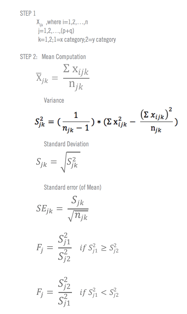
Related resources
Analysis & Reporting
Margin of error 11 min read
Data saturation in qualitative research 8 min read, thematic analysis 11 min read, behavioral analytics 12 min read, statistical significance calculator: tool & complete guide 18 min read, regression analysis 19 min read, data analysis 31 min read, request demo.
Ready to learn more about Qualtrics?
Microbe Notes
T-test: Definition, Formula, Types, Applications
The t-test is a test in statistics that is used for testing hypotheses regarding the mean of a small sample taken population when the standard deviation of the population is not known.
- The t-test is used to determine if there is a significant difference between the means of two groups.
- The t-test is used for hypothesis testing to determine whether a process has an effect on both samples or if the groups are different from each other.
- Basically, the t-test allows the comparison of the mean of two sets of data and the determination if the two sets are derived from the same population.
- After the null and alternative hypotheses are established, t-test formulas are used to calculate values that are then compared with standard values.
- Based on the comparison, the null hypothesis is either rejected or accepted.
- The T-test is similar to other tests like the z-test and f-test except that t-test is usually performed in cases where the sample size is small (n≤30).
Table of Contents
Interesting Science Videos
T-test Formula
T-tests can be performed manually using a formula or through some software.

One sample t-test (one-tailed t-test)
- One sample t-test is a statistical test where the critical area of a distribution is one-sided so that the alternative hypothesis is accepted if the population parameter is either greater than or less than a certain value, but not both.
- In the case where the t-score of the sample being tested falls into the critical area of a one-sided test, the alternative hypothesis is to be accepted instead of the null hypothesis.
- A one-tailed test is used to determine if the population is either lower than or higher than some hypothesized value.
- A one-tailed test is appropriate if the estimated value might depart from the sample value in either of the directions, left or right, but not both.

- For this test, the null hypothesis states that there is no difference between the true mean and the assumed value whereas the alternative hypothesis states that either the assumed value is greater than or less than the true mean but not both.
- For instance, if our H 0 : µ 0 = µ and H a : µ < µ 0 , such a test would be a one-sided test or more precisely, a left-tailed test.
- Under such conditions, there is one rejection area only on the left tail of the distribution.
- If we consider µ = 100 and if our sample mean deviates significantly from 100 towards the lower direction, H 0 or null hypothesis is rejected. Otherwise, H 0 is accepted at a given level of significance.
- Similarly, if in another case, H 0 : µ = µ 0 and H a : µ > µ 0 , this is also a one-tailed test (right tail) and the rejection region is present on the right tail of the curve.
- In this case, when µ = 100 and the sample mean deviates significantly from 100 in the upward direction, H 0 is rejected otherwise, it is to be accepted.
Two sample t-test (two-tailed t-test)
- Two sample t-test is a test a method in which the critical area of a distribution is two-sided and the test is performed to determine whether the population parameter of the sample is greater than or less than a specific range of values.
- A two-tailed test rejects the null hypothesis in cases where the sample mean is significantly higher or lower than the assumed value of the mean of the population.
- This type of test is appropriate when the null hypothesis is some assumed value, and the alternative hypothesis is set as the value not equal to the specified value of the null hypothesis.

- The two-tailed test is appropriate when we have H 0 : µ = µ 0 and H a : µ ≠ µ 0 which may mean µ > µ 0 or µ < µ 0 .
- Therefore, in a two-tailed test, there are two rejection regions, one in either direction, left and right, towards each tail of the curve.
- Suppose, we take µ = 100 and if our sample mean deviates significantly from 100 in either direction, the null hypothesis can be rejected. But if the sample mean does not deviate considerably from µ, the null hypothesis is accepted.
Independent t-test
- An Independent t-test is a test used for judging the means of two independent groups to determine the statistical evidence to prove that the population means are significantly different.
- Subjects in each sample are also assumed to come from different populations, that is, subjects in “Sample A” are assumed to come from “Population A” and subjects in “Sample B” are assumed to come from “Population B.”
- The populations are assumed to differ only in the level of the independent variable.
- Thus, any difference found between the sample means should also exist between population means, and any difference between the population means must be due to the difference in the levels of the independent variable.
- Based on this information, a curve can be plotted to determine the effect of an independent variable on the dependent variable and vice versa.
T-test Applications
- The T-test compares the mean of two samples, dependent or independent.
- It can also be used to determine if the sample mean is different from the assumed mean.
- T-test has an application in determining the confidence interval for a sample mean.
References and Sources
- R. Kothari (1990) Research Methodology. Vishwa Prakasan. India.
- 3% – https://www.investopedia.com/terms/o/one-tailed-test.asp
- 2% – https://towardsdatascience.com/hypothesis-testing-in-machine-learning-using-python-a0dc89e169ce
- 2% – https://en.wikipedia.org/wiki/Two-tailed_test
- 1% – https://www.scribbr.com/statistics/t-test/
- 1% – https://www.scalelive.com/null-hypothesis.html
- 1% – https://www.investopedia.com/terms/t/two-tailed-test.asp
- 1% – https://www.investopedia.com/ask/answers/073115/what-assumptions-are-made-when-conducting-ttest.asp
- 1% – https://www.chegg.com/homework-help/questions-and-answers/sample-100-steel-wires-average-breaking-strength-x-50-kn-standard-deviation-sigma-4-kn–fi-q20558661
- 1% – https://support.minitab.com/en-us/minitab/18/help-and-how-to/statistics/basic-statistics/supporting-topics/basics/null-and-alternative-hypotheses/
- 1% – https://libguides.library.kent.edu/SPSS/IndependentTTest
- 1% – https://keydifferences.com/difference-between-t-test-and-z-test.html
- 1% – https://keydifferences.com/difference-between-t-test-and-f-test.html
- 1% – http://www.sci.utah.edu/~arpaiva/classes/UT_ece3530/hypothesis_testing.pdf
- <1% – https://www.thoughtco.com/overview-of-the-demand-curve-1146962
- <1% – https://www.slideshare.net/aniket0013/formulating-hypotheses
- <1% – https://en.wikipedia.org/wiki/Null_hypothesis
About Author

Anupama Sapkota
2 thoughts on “T-test: Definition, Formula, Types, Applications”
Hi, on the very top, the one sample t-test formula in the picture is incorrect. It should be x-bar – u, not +
Thanks, it has been corrected 🙂
Leave a Comment Cancel reply
Save my name, email, and website in this browser for the next time I comment.
This site uses Akismet to reduce spam. Learn how your comment data is processed .

An official website of the United States government
The .gov means it’s official. Federal government websites often end in .gov or .mil. Before sharing sensitive information, make sure you’re on a federal government site.
The site is secure. The https:// ensures that you are connecting to the official website and that any information you provide is encrypted and transmitted securely.
- Publications
- Account settings
Preview improvements coming to the PMC website in October 2024. Learn More or Try it out now .
- Advanced Search
- Journal List
- Korean J Anesthesiol
- v.68(6); 2015 Dec
T test as a parametric statistic
Tae kyun kim.
Department of Anesthesia and Pain Medicine, Pusan National University School of Medicine, Busan, Korea.
In statistic tests, the probability distribution of the statistics is important. When samples are drawn from population N (µ, σ 2 ) with a sample size of n, the distribution of the sample mean X ̄ should be a normal distribution N (µ, σ 2 / n ). Under the null hypothesis µ = µ 0 , the distribution of statistics z = X ¯ - µ 0 σ / n should be standardized as a normal distribution. When the variance of the population is not known, replacement with the sample variance s 2 is possible. In this case, the statistics X ¯ - µ 0 s / n follows a t distribution ( n-1 degrees of freedom). An independent-group t test can be carried out for a comparison of means between two independent groups, with a paired t test for paired data. As the t test is a parametric test, samples should meet certain preconditions, such as normality, equal variances and independence.
Introduction
A t test is a type of statistical test that is used to compare the means of two groups. It is one of the most widely used statistical hypothesis tests in pain studies [ 1 ]. There are two types of statistical inference: parametric and nonparametric methods. Parametric methods refer to a statistical technique in which one defines the probability distribution of probability variables and makes inferences about the parameters of the distribution. In cases in which the probability distribution cannot be defined, nonparametric methods are employed. T tests are a type of parametric method; they can be used when the samples satisfy the conditions of normality, equal variance, and independence.
T tests can be divided into two types. There is the independent t test, which can be used when the two groups under comparison are independent of each other, and the paired t test, which can be used when the two groups under comparison are dependent on each other. T tests are usually used in cases where the experimental subjects are divided into two independent groups, with one group treated with A and the other group treated with B. Researchers can acquire two types of results for each group (i.e., prior to treatment and after the treatment): preA and postA, and preB and postB. An independent t test can be used for an intergroup comparison of postA and postB or for an intergroup comparison of changes in preA to postA (postA-preA) and changes in preB to postB (postB-preB) ( Table 1 ).
| Treatment A | Treatment B | |||||||
|---|---|---|---|---|---|---|---|---|
| ID | preA | postA | ΔA | ID | preB | postB | ΔB | |
| 1 | 63 | 77 | 14 | 11 | 81 | 101 | 20 | |
| 2 | 69 | 88 | 19 | 12 | 87 | 103 | 16 | |
| 3 | 76 | 90 | 14 | 13 | 77 | 107 | 30 | |
| 4 | 78 | 95 | 17 | 14 | 80 | 114 | 34 | |
| 5 | 80 | 96 | 16 | 15 | 76 | 116 | 40 | |
| 6 | 89 | 96 | 7 | 16 | 86 | 116 | 30 | |
| 7 | 90 | 102 | 12 | 17 | 98 | 116 | 18 | |
| 8 | 92 | 104 | 12 | 18 | 87 | 120 | 33 | |
| 9 | 103 | 110 | 7 | 19 | 105 | 120 | 15 | |
| 10 | 112 | 115 | 3 | 20 | 69 | 127 | 58 | |
ID: individual identification, preA, preB: before the treatment A or B, postA, postB: after the treatment A or B, ΔA, ΔB: difference between before and after the treatment A or B.
On the other hand, paired t tests are used in different experimental environments. For example, the experimental subjects are not divided into two groups, and all of them are treated initially with A. The amount of change (postA-preA) is then measured for all subjects. After all of the effects of A disappear, the subjects are treated with B, and the amount of change (postB-preB) is measured for all of the subjects. A paired t test is used in such crossover test designs to compare the amount of change of A to that of B for the same subjects ( Table 2 ).
| Treatment A | Treatment B | |||||||
|---|---|---|---|---|---|---|---|---|
| ID | preA | postA | ΔA | ID | preB | postB | ΔB | |
| 1 | 63 | 77 | 14 | 1 | 73 | 103 | 30 | |
| 2 | 69 | 88 | 19 | 2 | 74 | 104 | 30 | |
| 3 | 76 | 90 | 14 | 3 | 76 | 107 | 31 | |
| 4 | 78 | 95 | 17 | 4 | 84 | 108 | 24 | |
| 5 | 80 | 96 | 16 | wash out | 5 | 84 | 110 | 26 |
| 6 | 89 | 96 | 7 | 6 | 86 | 110 | 24 | |
| 7 | 90 | 102 | 12 | 7 | 92 | 113 | 21 | |
| 8 | 92 | 104 | 12 | 8 | 95 | 114 | 19 | |
| 9 | 103 | 110 | 7 | 9 | 103 | 118 | 15 | |
| 10 | 112 | 115 | 3 | 10 | 115 | 120 | 5 | |
Statistic and Probability
Statistics is basically about probabilities. A statistical conclusion of a large or small difference between two groups is not based on an absolute standard but is rather an evaluation of the probability of an event. For example, a clinical test is performed to determine whether or not a patient has a certain disease. If the test results are either higher or lower than the standard, clinicians will determine that the patient has the disease despite the fact that the patient may or may not actually have the disease. This conclusion is based on the statistical concept which holds that it is more statistically valid to conclude that the patient has the disease than to declare that the patient is a rare case among people without the disease because such test results are statistically rare in normal people.
The test results and the probability distribution of the results must be known in order for the results to be determined as statistically rare. The criteria for clinical indicators have been established based on data collected from an entire population or at least from a large number of people. Here, we examine a case in which a clinical indicator exhibits a normal distribution with a mean of µ and a variance of σ 2 . If a patient's test result is χ, is this statistically rare against the criteria (e.g., 5 or 1%)? Probability is represented as the surface area in a probability distribution, and the z score that represents either 5 or 1%, near the margins of the distribution, becomes the reference value. The test result χ can be determined to be statistically rare compared to the reference probability if it lies in a more marginal area than the z score, that is, if the value of χ is located in the marginal ends of the distribution ( Fig. 1 ).

This is done to compare one individual's clinical indicator value. This however raises the question of how we would compare the mean of a sample group (consisting of more than one individual) against the population mean. Again, it is meaningless to compare each individual separately; we must compare the means of the two groups. Thus, do we make a statistical inference using only the distribution of the clinical indicators of the entire population and the mean of the sample? No. In order to infer a statistical possibility, we must know the indicator of interest and its probability distribution. In other words, we must know the mean of the sample and the distribution of the mean. We can then determine how far the sample mean varies from the population mean by knowing the sampling distribution of the means.
Sampling Distribution (Sample Mean Distribution)
The sample mean we can get from a study is one of means of all possible samples which could be drawn from a population. This sample mean from a study was already acquired from a real experiment, however, how could we know the distribution of the means of all possible samples including studied sample? Do we need to experiment it over and over again? The simulation in which samples are drawn repeatedly from a population is shown in Fig. 2 . If samples are drawn with sample size n from population of normal distribution (µ, σ 2 ), the sampling distribution shows normal distribution with mean of µ and variance of σ 2 / n . The number of samples affects the shape of the sampling distribution. That is, the shape of the distribution curve becomes a narrower bell curve with a smaller variance as the number of samples increases, because the variance of sampling distribution is σ 2 / n . The formation of a sampling distribution is well explained in Lee et al. [ 2 ] in a form of a figure.

T Distribution
Now that the sampling distribution of the means is known, we can locate the position of the mean of a specific sample against the distribution data. However, one problem remains. As we noted earlier, the sampling distribution exhibits a normal distribution with a variance of σ 2 / n , but in reality we do not know σ 2 , the variance of the population. Therefore, we use the sample variance instead of the population variance to determine the sampling distribution of the mean. The sample variance is defined as follows:
In such cases in which the sample variance is used, the sampling distribution follows a t distribution that depends on the 0degree of freedom of each sample rather than a normal distribution ( Fig. 3 ).

Independent T test
A t test is also known as Student's t test. It is a statistical analysis technique that was developed by William Sealy Gosset in 1908 as a means to control the quality of dark beers. A t test used to test whether there is a difference between two independent sample means is not different from a t test used when there is only one sample (as mentioned earlier). However, if there is no difference in the two sample means, the difference will be close to zero. Therefore, in such cases, an additional statistical test should be performed to verify whether the difference could be said to be equal to zero.
Let's extract two independent samples from a population that displays a normal distribution and compute the difference between the means of the two samples. The difference between the sample means will not always be zero, even if the samples are extracted from the same population, because the sampling process is randomized, which results in a sample with a variety of combinations of subjects. We extracted two samples with a size of 6 from a population N (150, 5 2 ) and found the difference in the means. If this process is repeated 1,000 times, the sampling distribution exhibits the shape illustrated in Fig. 4 . When the distribution is displayed in terms of a histogram and a density line, it is almost identical to the theoretical sampling distribution: N(0, 2 × 5 2 /6) ( Fig. 4 ).

However, it is difficult to define the distribution of the difference in the two sample means because the variance of the population is unknown. If we use the variance of the sample instead, the distribution of the difference of the samples means would follow a t distribution. It should be noted, however, that the two samples display a normal distribution and have an equal variance because they were independently extracted from an identical population that has a normal distribution.
Under the assumption that the two samples display a normal distribution and have an equal variance, the t statistic is as follows:
population mean difference (µ 1 - µ 2 ) was assumed to be 0; thus:
The population variance was unknown and so a pooled variance of the two samples was used:
However, if the population variance is not equal, the t statistic of the t test would be
and the degree of freedom is calculated based on the Welch Satterthwaite equation.
It is apparent that if n 1 and n 2 are sufficiently large, the t statistic resembles a normal distribution ( Fig. 3 ).
A statistical test is performed to verify the position of the difference in the sample means in the sampling distribution of the mean ( Fig. 4 ). It is statistically very rare for the difference in two sample means to lie on the margins of the distribution. Therefore, if the difference does lie on the margins, it is statistically significant to conclude that the samples were extracted from two different populations, even if they were actually extracted from the same population.
Paired T test
Paired t tests are can be categorized as a type of t test for a single sample because they test the difference between two paired results. If there is no difference between the two treatments, the difference in the results would be close to zero; hence, the difference in the sample means used for a paired t test would be 0.
Let's go back to the sampling distribution that was used in the independent t test discussed earlier. The variance of the difference between two independent sample means was represented as the sum of each variance. If the samples were not independent, the variance of the difference of two variables A and B, Var (A-B), can be shown as follows,
where σ 1 2 is the variance of variable A, σ 2 2 is the variance of variable B, and ρ is the correlation coefficient for the two variables. In an independent t test, the correlation coefficient is 0 because the two groups are independent. Thus, it is logical to show the variance of the difference between the two variables simply as the sum of the two variances. However, for paired variables, the correlation coefficient may not equal 0. Thus, the t statistic for two dependent samples must be different, meaning the following t statistic,
must be changed. First, the number of samples are paired; thus, n 1 = n 2 = n , and their variance can be represented as s 1 2 + s 2 2 - 2ρ s 1 s 2 considering the correlation coefficient. Therefore, the t statistic for a paired t test is as follows:
In this equation, the t statistic is increased if the correlation coefficient is greater than 0 because the denominator becomes smaller, which increases the statistical power of the paired t test compared to that of an independent t test. On the other hand, if the correlation coefficient is less than 0, the statistical power is decreased and becomes lower than that of an independent t test. It is important to note that if one misunderstands this characteristic and uses an independent t test when the correlation coefficient is less than 0, the generated results would be incorrect, as the process ignores the paired experimental design.
Assumptions
As previously explained, if samples are extracted from a population that displays a normal distribution but the population variance is unknown, we can use the sample variance to examine the sampling distribution of the mean, which will resemble a t distribution. Therefore, in order to reach a statistical conclusion about a sample mean with a t distribution, certain conditions must be satisfied: the two samples for comparison must be independently sampled from the same population, satisfying the conditions of normality, equal variance, and independence.
Shapiro's test or the Kolmogorov-Smirnov test can be performed to verify the assumption of normality. If the condition of normality is not met, the Wilcoxon rank sum test (Mann-Whitney U test) is used for independent samples, and the Wilcoxon sign rank test is used for paired samples for an additional nonparametric test.
The condition of equal variance is verified using Levene's test or Bartlett's test. If the condition of equal variance is not met, nonparametric test can be performed or the following statistic which follows a t distribution can is used.
However, this statistics has different degree of freedom which was calculated by the Welch-Satterthwaite [ 3 , 4 ] equation.
Owing to user-friendly statistics software programs, the rich pool of statistics information on the Internet, and expert advice from statistics professionals at every hospital, using and processing statistics data is no longer an intractable task. However, it remains the researchers' responsibility to design experiments to fulfill all of the conditions of their statistic methods of choice and to ensure that their statistical assumptions are appropriate. In particular, parametric statistical methods confer reasonable statistical conclusions only when the statistical assumptions are fully met. Some researchers often regard these statistical assumptions inconvenient and neglect them. Even some statisticians argue on the basic assumptions, based on the central limit theory, that sampling distributions display a normal distribution regardless of the fact that the population distribution may or may not follow a normal distribution, and that t tests have sufficient statistical power even if they do not satisfy the condition of normality [ 5 ]. Moreover, they contend that the condition of equal variance is not so strict because even if there is a ninefold difference in the variance, the α level merely changes from 0.5 to 0.6 [ 6 ]. However, the arguments regarding the conditions of normality and the limit to which the condition of equal variance may be violated are still bones of contention. Therefore, researchers who unquestioningly accept these arguments and neglect the basic assumptions of a t test when submitting papers will face critical comments from editors. Moreover, it will be difficult to persuade the editors to neglect the basic assumptions regardless of how solid the evidence in the paper is. Hence, researchers should sufficiently test basic statistical assumptions and employ methods that are widely accepted so as to draw valid statistical conclusions.
The results of independent and paired t tests of the examples are illustrated in Tables 1 and 2. The tests were conducted using the SPSS Statistics Package (IBM® SPSS® Statistics 21, SPSS Inc., Chicago, IL, USA).
Independent T test (Table 1)

First, we need to examine the degree of normality by confirming the Kolmogorov-Smirnov or Shapiro-Wilk test in the second table. We can determine that the samples satisfy the condition of normality because the P value is greater than 0.05. Next, we check the results of Levene's test to examine the equality of variance. The P value is again greater than 0.05; hence, the condition of equal variance is also met. Finally, we read the significance probability for the "equal variance assumed" line. If the condition of equal variance is not met (i.e., if the P value is less than 0.05 for Levene's test), we reach a conclusion by referring to the significance probability for the "equal variance not assumed" line, or we perform a nonparametric test.
Paired T test (Table 2)

A paired t test is identical to a single-sample t test. Therefore, we test the normality of the difference in the amount of change for treatment A and treatment B (ΔA-ΔB). The normality is verified based on the results of Kolmogorov-Smirnov and Shapiro-Wilk tests, as shown in the second table. In conclusion, there is a significant difference between the two treatments (i.e., the P value is less than 0.001).

- Quality Improvement
- Talk To Minitab
What are T Values and P Values in Statistics?
Topics: Hypothesis Testing
If you’re not a statistician, looking through statistical output can sometimes make you feel a bit like Alice in Wonderland. Suddenly, you step into a fantastical world where strange and mysterious phantasms appear out of nowhere.
For example, consider the T and P in your t-test results.
“Curiouser and curiouser!” you might exclaim, like Alice, as you gaze at your output.

What are these values, really? Where do they come from? Even if you’ve used the p-value to interpret the statistical significance of your results umpteen times , its actual origin may remain murky to you.
T & P: The Tweedledee and Tweedledum of a T-test
T and P are inextricably linked. They go arm in arm, like Tweedledee and Tweedledum. Here's why.
When you perform a t-test, you're usually trying to find evidence of a significant difference between population means (2-sample t) or between the population mean and a hypothesized value (1-sample t). The t-value measures the size of the difference relative to the variation in your sample data . Put another way, T is simply the calculated difference represented in units of standard error. The greater the magnitude of T, the greater the evidence against the null hypothesis. This means there is greater evidence that there is a significant difference. The closer T is to 0, the more likely there isn't a significant difference.
Remember, the t-value in your output is calculated from only one sample from the entire population. It you took repeated random samples of data from the same population, you'd get slightly different t-values each time, due to random sampling error (which is really not a mistake of any kind–it's just the random variation expected in the data).
How different could you expect the t-values from many random samples from the same population to be? And how does the t-value from your sample data compare to those expected t-values?
You can use a t-distribution to find out.
Using a t-distribution to calculate probability
For the sake of illustration, assume that you're using a 1-sample t-test to determine whether the population mean is greater than a hypothesized value, such as 5, based on a sample of 20 observations, as shown in the above t-test output.
- In Minitab, choose Graph > Probability Distribution Plot .
- Select View Probability , then click OK .
- From Distribution , select t .
- In Degrees of freedom , enter 19 . (For a 1-sample t test, the degrees of freedom equals the sample size minus 1).
- Click Shaded Area . Select X Value . Select Right Tail .
- In X Value , enter 2.8 (the t-value), then click OK .
The highest part (peak) of the distribution curve shows you where you can expect most of the t-values to fall. Most of the time, you’d expect to get t-values close to 0. That makes sense, right? Because if you randomly select representative samples from a population, the mean of most of those random samples from the population should be close to the overall population mean, making their differences (and thus the calculated t-values) close to 0.
Ready for a demo of Minitab Statistical Software? Just ask!

T values, P values, and poker hands

In other words, the probability of obtaining a t-value of 2.8 or higher, when sampling from the same population (here, a population with a hypothesized mean of 5), is approximately 0.006.
How likely is that? Not very! For comparison, the probability of being dealt 3-of-a-kind in a 5-card poker hand is over three times as high (≈ 0.021).
Given that the probability of obtaining a t-value this high or higher when sampling from this population is so low, what’s more likely? It’s more likely this sample doesn’t come from this population (with the hypothesized mean of 5). It's much more likely that this sample comes from different population, one with a mean greater than 5.
To wit: Because the p-value is very low (< alpha level), you reject the null hypothesis and conclude that there's a statistically significant difference.
In this way, T and P are inextricably linked. Consider them simply different ways to quantify the "extremeness" of your results under the null hypothesis. You can’t change the value of one without changing the other.
The larger the absolute value of the t-value, the smaller the p-value, and the greater the evidence against the null hypothesis.(You can verify this by entering lower and higher t values for the t-distribution in step 6 above).
Try this two-tailed follow up...
The t-distribution example shown above is based on a one-tailed t-test to determine whether the mean of the population is greater than a hypothesized value. Therefore the t-distribution example shows the probability associated with the t-value of 2.8 only in one direction (the right tail of the distribution).
How would you use the t-distribution to find the p-value associated with a t-value of 2.8 for two-tailed t-test (in both directions)?
Hint: In Minitab, adjust the options in step 5 to find the probability for both tails. If you don't have a copy of Minitab, download a free 30-day trial version .

You Might Also Like
- Trust Center
© 2023 Minitab, LLC. All Rights Reserved.
- Terms of Use
- Privacy Policy
- Cookies Settings
- Skip to primary navigation
- Skip to main content
- Skip to primary sidebar
Institute for Digital Research and Education
What statistical analysis should I use? Statistical analyses using SPSS
Introduction.
This page shows how to perform a number of statistical tests using SPSS. Each section gives a brief description of the aim of the statistical test, when it is used, an example showing the SPSS commands and SPSS (often abbreviated) output with a brief interpretation of the output. You can see the page Choosing the Correct Statistical Test for a table that shows an overview of when each test is appropriate to use. In deciding which test is appropriate to use, it is important to consider the type of variables that you have (i.e., whether your variables are categorical, ordinal or interval and whether they are normally distributed), see What is the difference between categorical, ordinal and interval variables? for more information on this.
About the hsb data file
Most of the examples in this page will use a data file called hsb2, high school and beyond. This data file contains 200 observations from a sample of high school students with demographic information about the students, such as their gender ( female ), socio-economic status ( ses ) and ethnic background ( race ). It also contains a number of scores on standardized tests, including tests of reading ( read ), writing ( write ), mathematics ( math ) and social studies ( socst ). You can get the hsb data file by clicking on hsb2 .
One sample t-test
A one sample t-test allows us to test whether a sample mean (of a normally distributed interval variable) significantly differs from a hypothesized value. For example, using the hsb2 data file , say we wish to test whether the average writing score ( write ) differs significantly from 50. We can do this as shown below. t-test /testval = 50 /variable = write. The mean of the variable write for this particular sample of students is 52.775, which is statistically significantly different from the test value of 50. We would conclude that this group of students has a significantly higher mean on the writing test than 50.
One sample median test
A one sample median test allows us to test whether a sample median differs significantly from a hypothesized value. We will use the same variable, write , as we did in the one sample t-test example above, but we do not need to assume that it is interval and normally distributed (we only need to assume that write is an ordinal variable). nptests /onesample test (write) wilcoxon(testvalue = 50).

Binomial test
A one sample binomial test allows us to test whether the proportion of successes on a two-level categorical dependent variable significantly differs from a hypothesized value. For example, using the hsb2 data file , say we wish to test whether the proportion of females ( female ) differs significantly from 50%, i.e., from .5. We can do this as shown below. npar tests /binomial (.5) = female. The results indicate that there is no statistically significant difference (p = .229). In other words, the proportion of females in this sample does not significantly differ from the hypothesized value of 50%.
Chi-square goodness of fit
A chi-square goodness of fit test allows us to test whether the observed proportions for a categorical variable differ from hypothesized proportions. For example, let’s suppose that we believe that the general population consists of 10% Hispanic, 10% Asian, 10% African American and 70% White folks. We want to test whether the observed proportions from our sample differ significantly from these hypothesized proportions. npar test /chisquare = race /expected = 10 10 10 70. These results show that racial composition in our sample does not differ significantly from the hypothesized values that we supplied (chi-square with three degrees of freedom = 5.029, p = .170).
Two independent samples t-test
An independent samples t-test is used when you want to compare the means of a normally distributed interval dependent variable for two independent groups. For example, using the hsb2 data file , say we wish to test whether the mean for write is the same for males and females. t-test groups = female(0 1) /variables = write. Because the standard deviations for the two groups are similar (10.3 and 8.1), we will use the “equal variances assumed” test. The results indicate that there is a statistically significant difference between the mean writing score for males and females (t = -3.734, p = .000). In other words, females have a statistically significantly higher mean score on writing (54.99) than males (50.12). See also SPSS Learning Module: An overview of statistical tests in SPSS
Wilcoxon-Mann-Whitney test
The Wilcoxon-Mann-Whitney test is a non-parametric analog to the independent samples t-test and can be used when you do not assume that the dependent variable is a normally distributed interval variable (you only assume that the variable is at least ordinal). You will notice that the SPSS syntax for the Wilcoxon-Mann-Whitney test is almost identical to that of the independent samples t-test. We will use the same data file (the hsb2 data file ) and the same variables in this example as we did in the independent t-test example above and will not assume that write , our dependent variable, is normally distributed.
npar test /m-w = write by female(0 1). The results suggest that there is a statistically significant difference between the underlying distributions of the write scores of males and the write scores of females (z = -3.329, p = 0.001). See also FAQ: Why is the Mann-Whitney significant when the medians are equal?
Chi-square test
A chi-square test is used when you want to see if there is a relationship between two categorical variables. In SPSS, the chisq option is used on the statistics subcommand of the crosstabs command to obtain the test statistic and its associated p-value. Using the hsb2 data file , let’s see if there is a relationship between the type of school attended ( schtyp ) and students’ gender ( female ). Remember that the chi-square test assumes that the expected value for each cell is five or higher. This assumption is easily met in the examples below. However, if this assumption is not met in your data, please see the section on Fisher’s exact test below. crosstabs /tables = schtyp by female /statistic = chisq. These results indicate that there is no statistically significant relationship between the type of school attended and gender (chi-square with one degree of freedom = 0.047, p = 0.828). Let’s look at another example, this time looking at the linear relationship between gender ( female ) and socio-economic status ( ses ). The point of this example is that one (or both) variables may have more than two levels, and that the variables do not have to have the same number of levels. In this example, female has two levels (male and female) and ses has three levels (low, medium and high). crosstabs /tables = female by ses /statistic = chisq. Again we find that there is no statistically significant relationship between the variables (chi-square with two degrees of freedom = 4.577, p = 0.101). See also SPSS Learning Module: An Overview of Statistical Tests in SPSS
Fisher’s exact test
The Fisher’s exact test is used when you want to conduct a chi-square test but one or more of your cells has an expected frequency of five or less. Remember that the chi-square test assumes that each cell has an expected frequency of five or more, but the Fisher’s exact test has no such assumption and can be used regardless of how small the expected frequency is. In SPSS unless you have the SPSS Exact Test Module, you can only perform a Fisher’s exact test on a 2×2 table, and these results are presented by default. Please see the results from the chi squared example above.
One-way ANOVA
A one-way analysis of variance (ANOVA) is used when you have a categorical independent variable (with two or more categories) and a normally distributed interval dependent variable and you wish to test for differences in the means of the dependent variable broken down by the levels of the independent variable. For example, using the hsb2 data file , say we wish to test whether the mean of write differs between the three program types ( prog ). The command for this test would be: oneway write by prog. The mean of the dependent variable differs significantly among the levels of program type. However, we do not know if the difference is between only two of the levels or all three of the levels. (The F test for the Model is the same as the F test for prog because prog was the only variable entered into the model. If other variables had also been entered, the F test for the Model would have been different from prog .) To see the mean of write for each level of program type, means tables = write by prog. From this we can see that the students in the academic program have the highest mean writing score, while students in the vocational program have the lowest. See also SPSS Textbook Examples: Design and Analysis, Chapter 7 SPSS Textbook Examples: Applied Regression Analysis, Chapter 8 SPSS FAQ: How can I do ANOVA contrasts in SPSS? SPSS Library: Understanding and Interpreting Parameter Estimates in Regression and ANOVA
Kruskal Wallis test
The Kruskal Wallis test is used when you have one independent variable with two or more levels and an ordinal dependent variable. In other words, it is the non-parametric version of ANOVA and a generalized form of the Mann-Whitney test method since it permits two or more groups. We will use the same data file as the one way ANOVA example above (the hsb2 data file ) and the same variables as in the example above, but we will not assume that write is a normally distributed interval variable. npar tests /k-w = write by prog (1,3). If some of the scores receive tied ranks, then a correction factor is used, yielding a slightly different value of chi-squared. With or without ties, the results indicate that there is a statistically significant difference among the three type of programs.
Paired t-test
A paired (samples) t-test is used when you have two related observations (i.e., two observations per subject) and you want to see if the means on these two normally distributed interval variables differ from one another. For example, using the hsb2 data file we will test whether the mean of read is equal to the mean of write . t-test pairs = read with write (paired). These results indicate that the mean of read is not statistically significantly different from the mean of write (t = -0.867, p = 0.387).
Wilcoxon signed rank sum test
The Wilcoxon signed rank sum test is the non-parametric version of a paired samples t-test. You use the Wilcoxon signed rank sum test when you do not wish to assume that the difference between the two variables is interval and normally distributed (but you do assume the difference is ordinal). We will use the same example as above, but we will not assume that the difference between read and write is interval and normally distributed. npar test /wilcoxon = write with read (paired). The results suggest that there is not a statistically significant difference between read and write . If you believe the differences between read and write were not ordinal but could merely be classified as positive and negative, then you may want to consider a sign test in lieu of sign rank test. Again, we will use the same variables in this example and assume that this difference is not ordinal. npar test /sign = read with write (paired). We conclude that no statistically significant difference was found (p=.556).
McNemar test
You would perform McNemar’s test if you were interested in the marginal frequencies of two binary outcomes. These binary outcomes may be the same outcome variable on matched pairs (like a case-control study) or two outcome variables from a single group. Continuing with the hsb2 dataset used in several above examples, let us create two binary outcomes in our dataset: himath and hiread . These outcomes can be considered in a two-way contingency table. The null hypothesis is that the proportion of students in the himath group is the same as the proportion of students in hiread group (i.e., that the contingency table is symmetric). compute himath = (math>60). compute hiread = (read>60). execute. crosstabs /tables=himath BY hiread /statistic=mcnemar /cells=count. McNemar’s chi-square statistic suggests that there is not a statistically significant difference in the proportion of students in the himath group and the proportion of students in the hiread group.
One-way repeated measures ANOVA
You would perform a one-way repeated measures analysis of variance if you had one categorical independent variable and a normally distributed interval dependent variable that was repeated at least twice for each subject. This is the equivalent of the paired samples t-test, but allows for two or more levels of the categorical variable. This tests whether the mean of the dependent variable differs by the categorical variable. We have an example data set called rb4wide , which is used in Kirk’s book Experimental Design. In this data set, y is the dependent variable, a is the repeated measure and s is the variable that indicates the subject number. glm y1 y2 y3 y4 /wsfactor a(4). You will notice that this output gives four different p-values. The output labeled “sphericity assumed” is the p-value (0.000) that you would get if you assumed compound symmetry in the variance-covariance matrix. Because that assumption is often not valid, the three other p-values offer various corrections (the Huynh-Feldt, H-F, Greenhouse-Geisser, G-G and Lower-bound). No matter which p-value you use, our results indicate that we have a statistically significant effect of a at the .05 level. See also SPSS Textbook Examples from Design and Analysis: Chapter 16 SPSS Library: Advanced Issues in Using and Understanding SPSS MANOVA SPSS Code Fragment: Repeated Measures ANOVA
Repeated measures logistic regression
If you have a binary outcome measured repeatedly for each subject and you wish to run a logistic regression that accounts for the effect of multiple measures from single subjects, you can perform a repeated measures logistic regression. In SPSS, this can be done using the GENLIN command and indicating binomial as the probability distribution and logit as the link function to be used in the model. The exercise data file contains 3 pulse measurements from each of 30 people assigned to 2 different diet regiments and 3 different exercise regiments. If we define a “high” pulse as being over 100, we can then predict the probability of a high pulse using diet regiment. GET FILE='C:mydatahttps://stats.idre.ucla.edu/wp-content/uploads/2016/02/exercise.sav'. GENLIN highpulse (REFERENCE=LAST) BY diet (order = DESCENDING) /MODEL diet DISTRIBUTION=BINOMIAL LINK=LOGIT /REPEATED SUBJECT=id CORRTYPE = EXCHANGEABLE. These results indicate that diet is not statistically significant (Wald Chi-Square = 1.562, p = 0.211).
Factorial ANOVA
A factorial ANOVA has two or more categorical independent variables (either with or without the interactions) and a single normally distributed interval dependent variable. For example, using the hsb2 data file we will look at writing scores ( write ) as the dependent variable and gender ( female ) and socio-economic status ( ses ) as independent variables, and we will include an interaction of female by ses . Note that in SPSS, you do not need to have the interaction term(s) in your data set. Rather, you can have SPSS create it/them temporarily by placing an asterisk between the variables that will make up the interaction term(s). glm write by female ses. These results indicate that the overall model is statistically significant (F = 5.666, p = 0.00). The variables female and ses are also statistically significant (F = 16.595, p = 0.000 and F = 6.611, p = 0.002, respectively). However, that interaction between female and ses is not statistically significant (F = 0.133, p = 0.875). See also SPSS Textbook Examples from Design and Analysis: Chapter 10 SPSS FAQ: How can I do tests of simple main effects in SPSS? SPSS FAQ: How do I plot ANOVA cell means in SPSS? SPSS Library: An Overview of SPSS GLM
Friedman test
You perform a Friedman test when you have one within-subjects independent variable with two or more levels and a dependent variable that is not interval and normally distributed (but at least ordinal). We will use this test to determine if there is a difference in the reading, writing and math scores. The null hypothesis in this test is that the distribution of the ranks of each type of score (i.e., reading, writing and math) are the same. To conduct a Friedman test, the data need to be in a long format. SPSS handles this for you, but in other statistical packages you will have to reshape the data before you can conduct this test. npar tests /friedman = read write math. Friedman’s chi-square has a value of 0.645 and a p-value of 0.724 and is not statistically significant. Hence, there is no evidence that the distributions of the three types of scores are different.
Ordered logistic regression
Ordered logistic regression is used when the dependent variable is ordered, but not continuous. For example, using the hsb2 data file we will create an ordered variable called write3 . This variable will have the values 1, 2 and 3, indicating a low, medium or high writing score. We do not generally recommend categorizing a continuous variable in this way; we are simply creating a variable to use for this example. We will use gender ( female ), reading score ( read ) and social studies score ( socst ) as predictor variables in this model. We will use a logit link and on the print subcommand we have requested the parameter estimates, the (model) summary statistics and the test of the parallel lines assumption. if write ge 30 and write le 48 write3 = 1. if write ge 49 and write le 57 write3 = 2. if write ge 58 and write le 70 write3 = 3. execute. plum write3 with female read socst /link = logit /print = parameter summary tparallel. The results indicate that the overall model is statistically significant (p < .000), as are each of the predictor variables (p < .000). There are two thresholds for this model because there are three levels of the outcome variable. We also see that the test of the proportional odds assumption is non-significant (p = .563). One of the assumptions underlying ordinal logistic (and ordinal probit) regression is that the relationship between each pair of outcome groups is the same. In other words, ordinal logistic regression assumes that the coefficients that describe the relationship between, say, the lowest versus all higher categories of the response variable are the same as those that describe the relationship between the next lowest category and all higher categories, etc. This is called the proportional odds assumption or the parallel regression assumption. Because the relationship between all pairs of groups is the same, there is only one set of coefficients (only one model). If this was not the case, we would need different models (such as a generalized ordered logit model) to describe the relationship between each pair of outcome groups. See also SPSS Data Analysis Examples: Ordered logistic regression SPSS Annotated Output: Ordinal Logistic Regression
Factorial logistic regression
A factorial logistic regression is used when you have two or more categorical independent variables but a dichotomous dependent variable. For example, using the hsb2 data file we will use female as our dependent variable, because it is the only dichotomous variable in our data set; certainly not because it common practice to use gender as an outcome variable. We will use type of program ( prog ) and school type ( schtyp ) as our predictor variables. Because prog is a categorical variable (it has three levels), we need to create dummy codes for it. SPSS will do this for you by making dummy codes for all variables listed after the keyword with . SPSS will also create the interaction term; simply list the two variables that will make up the interaction separated by the keyword by . logistic regression female with prog schtyp prog by schtyp /contrast(prog) = indicator(1). The results indicate that the overall model is not statistically significant (LR chi2 = 3.147, p = 0.677). Furthermore, none of the coefficients are statistically significant either. This shows that the overall effect of prog is not significant. See also Annotated output for logistic regression
Correlation
A correlation is useful when you want to see the relationship between two (or more) normally distributed interval variables. For example, using the hsb2 data file we can run a correlation between two continuous variables, read and write . correlations /variables = read write. In the second example, we will run a correlation between a dichotomous variable, female , and a continuous variable, write . Although it is assumed that the variables are interval and normally distributed, we can include dummy variables when performing correlations. correlations /variables = female write. In the first example above, we see that the correlation between read and write is 0.597. By squaring the correlation and then multiplying by 100, you can determine what percentage of the variability is shared. Let’s round 0.597 to be 0.6, which when squared would be .36, multiplied by 100 would be 36%. Hence read shares about 36% of its variability with write . In the output for the second example, we can see the correlation between write and female is 0.256. Squaring this number yields .065536, meaning that female shares approximately 6.5% of its variability with write . See also Annotated output for correlation SPSS Learning Module: An Overview of Statistical Tests in SPSS SPSS FAQ: How can I analyze my data by categories? Missing Data in SPSS
Simple linear regression
Simple linear regression allows us to look at the linear relationship between one normally distributed interval predictor and one normally distributed interval outcome variable. For example, using the hsb2 data file , say we wish to look at the relationship between writing scores ( write ) and reading scores ( read ); in other words, predicting write from read . regression variables = write read /dependent = write /method = enter. We see that the relationship between write and read is positive (.552) and based on the t-value (10.47) and p-value (0.000), we would conclude this relationship is statistically significant. Hence, we would say there is a statistically significant positive linear relationship between reading and writing. See also Regression With SPSS: Chapter 1 – Simple and Multiple Regression Annotated output for regression SPSS Textbook Examples: Introduction to the Practice of Statistics, Chapter 10 SPSS Textbook Examples: Regression with Graphics, Chapter 2 SPSS Textbook Examples: Applied Regression Analysis, Chapter 5
Non-parametric correlation
A Spearman correlation is used when one or both of the variables are not assumed to be normally distributed and interval (but are assumed to be ordinal). The values of the variables are converted in ranks and then correlated. In our example, we will look for a relationship between read and write . We will not assume that both of these variables are normal and interval. nonpar corr /variables = read write /print = spearman. The results suggest that the relationship between read and write (rho = 0.617, p = 0.000) is statistically significant.
Simple logistic regression
Logistic regression assumes that the outcome variable is binary (i.e., coded as 0 and 1). We have only one variable in the hsb2 data file that is coded 0 and 1, and that is female . We understand that female is a silly outcome variable (it would make more sense to use it as a predictor variable), but we can use female as the outcome variable to illustrate how the code for this command is structured and how to interpret the output. The first variable listed after the logistic command is the outcome (or dependent) variable, and all of the rest of the variables are predictor (or independent) variables. In our example, female will be the outcome variable, and read will be the predictor variable. As with OLS regression, the predictor variables must be either dichotomous or continuous; they cannot be categorical. logistic regression female with read. The results indicate that reading score ( read ) is not a statistically significant predictor of gender (i.e., being female), Wald = .562, p = 0.453. Likewise, the test of the overall model is not statistically significant, LR chi-squared – 0.56, p = 0.453. See also Annotated output for logistic regression SPSS Library: What kind of contrasts are these?
Multiple regression
Multiple regression is very similar to simple regression, except that in multiple regression you have more than one predictor variable in the equation. For example, using the hsb2 data file we will predict writing score from gender ( female ), reading, math, science and social studies ( socst ) scores. regression variable = write female read math science socst /dependent = write /method = enter. The results indicate that the overall model is statistically significant (F = 58.60, p = 0.000). Furthermore, all of the predictor variables are statistically significant except for read . See also Regression with SPSS: Chapter 1 – Simple and Multiple Regression Annotated output for regression SPSS Frequently Asked Questions SPSS Textbook Examples: Regression with Graphics, Chapter 3 SPSS Textbook Examples: Applied Regression Analysis
Analysis of covariance
Analysis of covariance is like ANOVA, except in addition to the categorical predictors you also have continuous predictors as well. For example, the one way ANOVA example used write as the dependent variable and prog as the independent variable. Let’s add read as a continuous variable to this model, as shown below. glm write with read by prog. The results indicate that even after adjusting for reading score ( read ), writing scores still significantly differ by program type ( prog ), F = 5.867, p = 0.003. See also SPSS Textbook Examples from Design and Analysis: Chapter 14 SPSS Library: An Overview of SPSS GLM SPSS Library: How do I handle interactions of continuous and categorical variables?
Multiple logistic regression
Multiple logistic regression is like simple logistic regression, except that there are two or more predictors. The predictors can be interval variables or dummy variables, but cannot be categorical variables. If you have categorical predictors, they should be coded into one or more dummy variables. We have only one variable in our data set that is coded 0 and 1, and that is female . We understand that female is a silly outcome variable (it would make more sense to use it as a predictor variable), but we can use female as the outcome variable to illustrate how the code for this command is structured and how to interpret the output. The first variable listed after the logistic regression command is the outcome (or dependent) variable, and all of the rest of the variables are predictor (or independent) variables (listed after the keyword with ). In our example, female will be the outcome variable, and read and write will be the predictor variables. logistic regression female with read write. These results show that both read and write are significant predictors of female . See also Annotated output for logistic regression SPSS Textbook Examples: Applied Logistic Regression, Chapter 2 SPSS Code Fragments: Graphing Results in Logistic Regression
Discriminant analysis
Discriminant analysis is used when you have one or more normally distributed interval independent variables and a categorical dependent variable. It is a multivariate technique that considers the latent dimensions in the independent variables for predicting group membership in the categorical dependent variable. For example, using the hsb2 data file , say we wish to use read , write and math scores to predict the type of program a student belongs to ( prog ). discriminate groups = prog(1, 3) /variables = read write math. Clearly, the SPSS output for this procedure is quite lengthy, and it is beyond the scope of this page to explain all of it. However, the main point is that two canonical variables are identified by the analysis, the first of which seems to be more related to program type than the second. See also discriminant function analysis SPSS Library: A History of SPSS Statistical Features
One-way MANOVA
MANOVA (multivariate analysis of variance) is like ANOVA, except that there are two or more dependent variables. In a one-way MANOVA, there is one categorical independent variable and two or more dependent variables. For example, using the hsb2 data file , say we wish to examine the differences in read , write and math broken down by program type ( prog ). glm read write math by prog. The students in the different programs differ in their joint distribution of read , write and math . See also SPSS Library: Advanced Issues in Using and Understanding SPSS MANOVA GLM: MANOVA and MANCOVA SPSS Library: MANOVA and GLM
Multivariate multiple regression
Multivariate multiple regression is used when you have two or more dependent variables that are to be predicted from two or more independent variables. In our example using the hsb2 data file , we will predict write and read from female , math , science and social studies ( socst ) scores. glm write read with female math science socst. These results show that all of the variables in the model have a statistically significant relationship with the joint distribution of write and read .
Canonical correlation
Canonical correlation is a multivariate technique used to examine the relationship between two groups of variables. For each set of variables, it creates latent variables and looks at the relationships among the latent variables. It assumes that all variables in the model are interval and normally distributed. SPSS requires that each of the two groups of variables be separated by the keyword with . There need not be an equal number of variables in the two groups (before and after the with ). manova read write with math science /discrim. * * * * * * A n a l y s i s o f V a r i a n c e -- design 1 * * * * * * EFFECT .. WITHIN CELLS Regression Multivariate Tests of Significance (S = 2, M = -1/2, N = 97 ) Test Name Value Approx. F Hypoth. DF Error DF Sig. of F Pillais .59783 41.99694 4.00 394.00 .000 Hotellings 1.48369 72.32964 4.00 390.00 .000 Wilks .40249 56.47060 4.00 392.00 .000 Roys .59728 Note.. F statistic for WILKS' Lambda is exact. - - - - - - - - - - - - - - - - - - - - - - - - - - - - - - - - - - - - - EFFECT .. WITHIN CELLS Regression (Cont.) Univariate F-tests with (2,197) D. F. Variable Sq. Mul. R Adj. R-sq. Hypoth. MS Error MS F READ .51356 .50862 5371.66966 51.65523 103.99081 WRITE .43565 .42992 3894.42594 51.21839 76.03569 Variable Sig. of F READ .000 WRITE .000 - - - - - - - - - - - - - - - - - - - - - - - - - - - - - - - - - - - - - Raw canonical coefficients for DEPENDENT variables Function No. Variable 1 READ .063 WRITE .049 - - - - - - - - - - - - - - - - - - - - - - - - - - - - - - - - - - - - - Standardized canonical coefficients for DEPENDENT variables Function No. Variable 1 READ .649 WRITE .467 * * * * * * A n a l y s i s o f V a r i a n c e -- design 1 * * * * * * Correlations between DEPENDENT and canonical variables Function No. Variable 1 READ .927 WRITE .854 - - - - - - - - - - - - - - - - - - - - - - - - - - - - - - - - - - - - - Variance in dependent variables explained by canonical variables CAN. VAR. Pct Var DE Cum Pct DE Pct Var CO Cum Pct CO 1 79.441 79.441 47.449 47.449 - - - - - - - - - - - - - - - - - - - - - - - - - - - - - - - - - - - - - Raw canonical coefficients for COVARIATES Function No. COVARIATE 1 MATH .067 SCIENCE .048 - - - - - - - - - - - - - - - - - - - - - - - - - - - - - - - - - - - - - Standardized canonical coefficients for COVARIATES CAN. VAR. COVARIATE 1 MATH .628 SCIENCE .478 - - - - - - - - - - - - - - - - - - - - - - - - - - - - - - - - - - - - - Correlations between COVARIATES and canonical variables CAN. VAR. Covariate 1 MATH .929 SCIENCE .873 * * * * * * A n a l y s i s o f V a r i a n c e -- design 1 * * * * * * Variance in covariates explained by canonical variables CAN. VAR. Pct Var DE Cum Pct DE Pct Var CO Cum Pct CO 1 48.544 48.544 81.275 81.275 - - - - - - - - - - - - - - - - - - - - - - - - - - - - - - - - - - - - - Regression analysis for WITHIN CELLS error term --- Individual Univariate .9500 confidence intervals Dependent variable .. READ reading score COVARIATE B Beta Std. Err. t-Value Sig. of t MATH .48129 .43977 .070 6.868 .000 SCIENCE .36532 .35278 .066 5.509 .000 COVARIATE Lower -95% CL- Upper MATH .343 .619 SCIENCE .235 .496 Dependent variable .. WRITE writing score COVARIATE B Beta Std. Err. t-Value Sig. of t MATH .43290 .42787 .070 6.203 .000 SCIENCE .28775 .30057 .066 4.358 .000 COVARIATE Lower -95% CL- Upper MATH .295 .571 SCIENCE .158 .418 - - - - - - - - - - - - - - - - - - - - - - - - - - - - - - - - - - - - - * * * * * * A n a l y s i s o f V a r i a n c e -- design 1 * * * * * * EFFECT .. CONSTANT Multivariate Tests of Significance (S = 1, M = 0, N = 97 ) Test Name Value Exact F Hypoth. DF Error DF Sig. of F Pillais .11544 12.78959 2.00 196.00 .000 Hotellings .13051 12.78959 2.00 196.00 .000 Wilks .88456 12.78959 2.00 196.00 .000 Roys .11544 Note.. F statistics are exact. - - - - - - - - - - - - - - - - - - - - - - - - - - - - - - - - - - - - - EFFECT .. CONSTANT (Cont.) Univariate F-tests with (1,197) D. F. Variable Hypoth. SS Error SS Hypoth. MS Error MS F Sig. of F READ 336.96220 10176.0807 336.96220 51.65523 6.52329 .011 WRITE 1209.88188 10090.0231 1209.88188 51.21839 23.62202 .000 - - - - - - - - - - - - - - - - - - - - - - - - - - - - - - - - - - - - - EFFECT .. CONSTANT (Cont.) Raw discriminant function coefficients Function No. Variable 1 READ .041 WRITE .124 - - - - - - - - - - - - - - - - - - - - - - - - - - - - - - - - - - - - - Standardized discriminant function coefficients Function No. Variable 1 READ .293 WRITE .889 - - - - - - - - - - - - - - - - - - - - - - - - - - - - - - - - - - - - - Estimates of effects for canonical variables Canonical Variable Parameter 1 1 2.196 * * * * * * A n a l y s i s o f V a r i a n c e -- design 1 * * * * * * EFFECT .. CONSTANT (Cont.) Correlations between DEPENDENT and canonical variables Canonical Variable Variable 1 READ .504 WRITE .959 - - - - - - - - - - - - - - - - - - - - - - - - - - - - - - - - - - - - - The output above shows the linear combinations corresponding to the first canonical correlation. At the bottom of the output are the two canonical correlations. These results indicate that the first canonical correlation is .7728. The F-test in this output tests the hypothesis that the first canonical correlation is equal to zero. Clearly, F = 56.4706 is statistically significant. However, the second canonical correlation of .0235 is not statistically significantly different from zero (F = 0.1087, p = 0.7420).
Factor analysis
Factor analysis is a form of exploratory multivariate analysis that is used to either reduce the number of variables in a model or to detect relationships among variables. All variables involved in the factor analysis need to be interval and are assumed to be normally distributed. The goal of the analysis is to try to identify factors which underlie the variables. There may be fewer factors than variables, but there may not be more factors than variables. For our example using the hsb2 data file , let’s suppose that we think that there are some common factors underlying the various test scores. We will include subcommands for varimax rotation and a plot of the eigenvalues. We will use a principal components extraction and will retain two factors. (Using these options will make our results compatible with those from SAS and Stata and are not necessarily the options that you will want to use.) factor /variables read write math science socst /criteria factors(2) /extraction pc /rotation varimax /plot eigen. Communality (which is the opposite of uniqueness) is the proportion of variance of the variable (i.e., read ) that is accounted for by all of the factors taken together, and a very low communality can indicate that a variable may not belong with any of the factors. The scree plot may be useful in determining how many factors to retain. From the component matrix table, we can see that all five of the test scores load onto the first factor, while all five tend to load not so heavily on the second factor. The purpose of rotating the factors is to get the variables to load either very high or very low on each factor. In this example, because all of the variables loaded onto factor 1 and not on factor 2, the rotation did not aid in the interpretation. Instead, it made the results even more difficult to interpret. See also SPSS FAQ: What does Cronbach’s alpha mean?
Your Name (required)
Your Email (must be a valid email for us to receive the report!)
Comment/Error Report (required)
How to cite this page
- © 2021 UC REGENTS
- Download PDF
- CME & MOC
- Share X Facebook Email LinkedIn
- Permissions
Test-Negative Study Designs for Evaluating Vaccine Effectiveness
- 1 Department of Biostatistics and Bioinformatics, Rollins School of Public Health, Emory University, Atlanta, Georgia
- Original Investigation Association Between 3 Doses of mRNA COVID-19 Vaccine and Symptomatic Infection Caused by Omicron and Delta Variants Emma K. Accorsi, PhD; Amadea Britton, MD; Katherine E. Fleming-Dutra, MD; Zachary R. Smith, MA; Nong Shang, PhD; Gordana Derado, PhD; Joseph Miller, PhD; Stephanie J. Schrag, DPhil; Jennifer R. Verani, MD, MPH JAMA
The evaluation of vaccines continues long after initial regulatory approval. Postapproval observational studies are often used to investigate aspects of vaccine effectiveness (VE) that clinical trials cannot feasibly assess. These includes long-term effectiveness, effectiveness within subgroups, effectiveness against rare outcomes, and effectiveness as the circulating pathogen changes. 1 Policymakers rely on these data to guide vaccine recommendations or formulation updates. 2
Read More About
Dean N , Amin AB. Test-Negative Study Designs for Evaluating Vaccine Effectiveness. JAMA. Published online June 12, 2024. doi:10.1001/jama.2024.5633
Manage citations:
© 2024
Artificial Intelligence Resource Center
Cardiology in JAMA : Read the Latest
Browse and subscribe to JAMA Network podcasts!
Others Also Liked
Select your interests.
Customize your JAMA Network experience by selecting one or more topics from the list below.
- Academic Medicine
- Acid Base, Electrolytes, Fluids
- Allergy and Clinical Immunology
- American Indian or Alaska Natives
- Anesthesiology
- Anticoagulation
- Art and Images in Psychiatry
- Artificial Intelligence
- Assisted Reproduction
- Bleeding and Transfusion
- Caring for the Critically Ill Patient
- Challenges in Clinical Electrocardiography
- Climate and Health
- Climate Change
- Clinical Challenge
- Clinical Decision Support
- Clinical Implications of Basic Neuroscience
- Clinical Pharmacy and Pharmacology
- Complementary and Alternative Medicine
- Consensus Statements
- Coronavirus (COVID-19)
- Critical Care Medicine
- Cultural Competency
- Dental Medicine
- Dermatology
- Diabetes and Endocrinology
- Diagnostic Test Interpretation
- Drug Development
- Electronic Health Records
- Emergency Medicine
- End of Life, Hospice, Palliative Care
- Environmental Health
- Equity, Diversity, and Inclusion
- Facial Plastic Surgery
- Gastroenterology and Hepatology
- Genetics and Genomics
- Genomics and Precision Health
- Global Health
- Guide to Statistics and Methods
- Hair Disorders
- Health Care Delivery Models
- Health Care Economics, Insurance, Payment
- Health Care Quality
- Health Care Reform
- Health Care Safety
- Health Care Workforce
- Health Disparities
- Health Inequities
- Health Policy
- Health Systems Science
- History of Medicine
- Hypertension
- Images in Neurology
- Implementation Science
- Infectious Diseases
- Innovations in Health Care Delivery
- JAMA Infographic
- Law and Medicine
- Leading Change
- Less is More
- LGBTQIA Medicine
- Lifestyle Behaviors
- Medical Coding
- Medical Devices and Equipment
- Medical Education
- Medical Education and Training
- Medical Journals and Publishing
- Mobile Health and Telemedicine
- Narrative Medicine
- Neuroscience and Psychiatry
- Notable Notes
- Nutrition, Obesity, Exercise
- Obstetrics and Gynecology
- Occupational Health
- Ophthalmology
- Orthopedics
- Otolaryngology
- Pain Medicine
- Palliative Care
- Pathology and Laboratory Medicine
- Patient Care
- Patient Information
- Performance Improvement
- Performance Measures
- Perioperative Care and Consultation
- Pharmacoeconomics
- Pharmacoepidemiology
- Pharmacogenetics
- Pharmacy and Clinical Pharmacology
- Physical Medicine and Rehabilitation
- Physical Therapy
- Physician Leadership
- Population Health
- Primary Care
- Professional Well-being
- Professionalism
- Psychiatry and Behavioral Health
- Public Health
- Pulmonary Medicine
- Regulatory Agencies
- Reproductive Health
- Research, Methods, Statistics
- Resuscitation
- Rheumatology
- Risk Management
- Scientific Discovery and the Future of Medicine
- Shared Decision Making and Communication
- Sleep Medicine
- Sports Medicine
- Stem Cell Transplantation
- Substance Use and Addiction Medicine
- Surgical Innovation
- Surgical Pearls
- Teachable Moment
- Technology and Finance
- The Art of JAMA
- The Arts and Medicine
- The Rational Clinical Examination
- Tobacco and e-Cigarettes
- Translational Medicine
- Trauma and Injury
- Treatment Adherence
- Ultrasonography
- Users' Guide to the Medical Literature
- Vaccination
- Venous Thromboembolism
- Veterans Health
- Women's Health
- Workflow and Process
- Wound Care, Infection, Healing
- Register for email alerts with links to free full-text articles
- Access PDFs of free articles
- Manage your interests
- Save searches and receive search alerts
Learn / Guides / Usability testing guide
Back to guides
Usability testing: your 101 introduction
A multi-chapter look at website usability testing, its benefits and methods, and how to get started with it.
Last updated
Reading time, take your first usability testing step today.
Sign up for a free Hotjar account and make sure your site behaves as you intend it to.
Usability testing is all about getting real people to interact with a website, app, or other product you've built and observing their behavior and reactions to it. Whether you start small by watching session recordings or go all out and rent a lab with eye-tracking equipment, usability testing is a necessary step to make sure you build an effective, efficient, and enjoyable experience for your users.
We start this guide with an introduction to:
What is usability testing
Why usability testing matters
What are the benefits of usability testing
What is not usability testing
The following chapters cover different testing methods , the usability questions they can help you answer, how to run a usability testing session , how to analyze and evaluate your testing results. Finally, we wrap up with 12 checklists and templates to help you run efficient usability sessions, and the best usability testing tools .
What is usability testing?
Usability testing is a method of testing the functionality of a website, app, or other digital product by observing real users as they attempt to complete tasks on it . The users are usually observed by researchers working for a business during either an in-person or, more commonly, a remote usability testing session.
The goal of usability testing is to reveal areas of confusion and uncover pain points in the customer journey to highlight opportunities to improve the overall user experience. Usability evaluation seeks to gauge the practical functionality of the product, specifically how efficiently a user completes a pre-defined goal.
(Note: if all testing activities take place on a website, the terms 'usability testing' and ' website usability testing' can be used interchangeably—which is what we're going to do throughout the rest of this page.)
💡Did you know there are different types of usability tests ?
Moderated usability testing : a facilitator introduces the test to participants, answers their queries, and asks follow-up questions
Unmoderated usability testing : the participants conduct the test without direct supervision, usually with a script
Remote usability testing : the test participants (and the researcher, in the case of moderated usability testing) conduct the test online or, more rarely, over the phone
In-person usability testing : the test participants and the researcher(s) are in the same location
Hotjar Engage lets you conduct remote, moderated usability testing with your own users or testers from our pool of 175,000+ participants.

What is the difference between usability testing and user testing?
While the terms are often used interchangeably, usability testing and user testing differ in scope.
They are both, however, a part of UX testing—a more comprehensive approach aiming to analyze the user experience at every touchpoint, including users’ perception of a digital product or service’s performance, emotional response, perceived value, and satisfaction with UX design, as well as their overall impression of the company and brand.

User testing is a research method that uses real people to evaluate a product or service by observing their interactions and gathering feedback.
By comparison with usability testing, user testing insights reveal:
What users think about when using your product or service
How they perceive your product or service
What are their user needs
Usability testing, on the other hand, has a more focused approached, by seeking to answer questions like:
Are there bugs or other errors impacting user flow?
Can users complete their task efficiently?
Do they understand how to navigate the site?
Why is usability testing important?
Usability testing is done by real-life users who are likely to reveal issues that people familiar with a website can no longer identify—very often, in-depth knowledge makes it easy for designers, marketers, and product owners to miss a website's usability issues.
Bringing in new users to test your site and/or observing how real people are already using it are effective ways to determine whether your visitors:
Understand how your site works and don't get 'lost' or confused
Can complete the main actions they need to
Don't encounter usability issues or bugs
Have a functional and efficient experience
Notice any other usability problems
This type of user research is exceptionally important with new products or new design updates: without it, you may be stuck with a UX design process that your team members understand, but your target audience will not.
I employ usability testing when I’m looking to gut-check myself as a designer. Sometimes I run designs by my cross-functional squad or the design team and we all have conflicting feedback. The catch is, we’re not always our user so it’s hard to sift through and agree on the best way forward.
Usability testing cuts through the noise and reveals if the usability of a proposed design meets basic expectations. It’s a great way to quickly de-risk engineering investment.
I also like to iterate on designs as we receive more and more information, so usability testing is a great way to move fast and not break too many things in the process.
Top 8 benefits of website usability testing
Your website can benefit from usability testing no matter where it is in the development process, from prototyping all the way to the finished product. You can also continue to test the user experience as you iterate and improve your product over time.
Employing tests with real users helps you:
Validate your prototype . Bring in users in the early stages of the development process, and test whether they’re experiencing any issues before locking down a final product. Do they encounter any bugs ? Does your site or product behave as expected when users interact with it? Testing on a prototype first can validate your concept and help you make plans for future functionality before you spend a lot of money to build out a complete website.
Confirm your product meets expectations. Once your product is completed, test usability again to make sure everything works the way it was intended. How's the ease of use? Is something still missing in the interface?
Identify issues with complex flows . If there are functions on your site that need users to follow multiple steps (for example an ecommerce checkout process ), run usability testing to make sure these processes are as straightforward and intuitive as possible.
Complement and illuminate other data points . Usability testing can often provide the why behind data points accumulated from other methods: your funnel analysis might show you that visitors drop off your site , and conducting usability testing can highlight underlying issues with pages with high churn rate.
Catch minor errors . In addition to large-scale usability issues, usability testing can help identify smaller errors. A new set of eyes is more likely to pick up on broken links, site errors, and grammatical issues that have been inadvertently glossed over. Usability testing can also validate fixes made after identifying those errors.
💡Pro tip: enable console tracking in Hotjar and filter session recordings by ‘Error’ to watch sessions of users who ran into a JavaScript error.
Open the console from the recording player to understand where the issue comes from, fix the issue, and run a usability test to validate the fix.
Develop empathy. It's not unusual for the people working on a project to develop tunnel vision around their product and forget they have access to knowledge that their typical website visitor may not have. Usability testing is a good way to develop some empathy for the real people who are using and will be using your site, and look at things from their perspective.
Get buy-in for change. It's one thing to know about a website issue; it's another to see users actually struggle with it. When it's evident that something is being misunderstood by users, it's natural to want to make it right. Watching short clips of key usability testing findings can be a very persuasive way to lobby for change within your organization.
Ultimately provide a better user experience. Great customer experience is essential for a successful product. Usability testing can help you identify issues that wouldn't be uncovered otherwise and create the most user-friendly product possible.
What usability testing is not
There are several UX tools and user testing tools that help improve the customer experience , but don't really qualify as 'usability testing tools' because they don't explicitly evaluate the functionality of a product:
A/B testing : A/B testing is a way to experiment with multiple versions of a web page to see which is most effective. While it can be used to test changes based on user testing, it is not a usability testing tool.
Focus groups : focus groups are a type of user testing , for which researchers gather a group of people together to discuss a specific topic. Usually, the goal is to learn people's opinions about a product or service, not to test how they use it.
Surveys : use surveys to gauge user experience. Because they do not allow you to actually observe visitors on the site in action, surveys are not considered usability testing—though they may be used in conjunction with it via a website usability survey .
Heatmaps : heatmaps offer a visual representation of how users interact with the page by showing the hottest (most engaged with) and coolest (least engaged with) parts of it. The click , scroll , and move maps allow you to see how users in aggregate engage with a website, but they are still technically not usability testing.
User acceptance testing : this is often the last phase of the software-testing process, where testers go through a calibrated set of steps to ensure the software works correctly. This is a technical test of QA (quality assurance), not a way to evaluate if the product is user-friendly and efficient.
In-house proper use testing : people in your company probably test software all the time, but this is not usability testing. Employees are inherently biased, making them unable to give the kind of honest results that real users can.
How to get started
Your website's user interface should be straightforward and easy to use, and usability testing is an essential step in getting there. But to get the most actionable results, testing must be done correctly—you will need to reproduce normal-use conditions exactly.
One of the easiest ways to get started with usability testing is through session recordings . Observing how visitors navigate your website can help you create the best user experience possible.
Frequently asked questions about usability testing
What is website usability testing.
Website usability testing is the practice of evaluating the functionality of your website by observing visitors’ actions and behavior as they complete specific tasks. Website usability testing lets you experience your site from the visitors’ perspective so you can identify opportunities to improve the user experience.
What is the purpose of usability testing?
Your in-depth knowledge of, and familiarity with, your website might prevent you from seeing its design or usability issues. When you run a website usability test, users can identify issues with your site that you may have otherwise missed. For example website bugs , missing or broken elements, or an ineffective call to action (CTA) .
What are some types of website usability tests?
The type of website usability test you need will be based on your available resources, target audience, and goals. The main types of usability tests are:
Remote or in-person
Moderated or unmoderated
Scripted or unscripted
For more detailed information about the types of usability tests and to determine which one you should try on your site, visit the usability testing methods chapter of this guide.
How do you run a usability test on a website?
Your goals and objectives will determine both the steps you’ll need to take to run a test on your website and the usability testing questions you’ll ask.
Having a plan before you start will help you organize the data and results you collect in an understandable way so you can improve the user experience. These 12 usability testing checklists and templates are a good place to start.
A 5-step process for moderated usability testing could be:
Plan the session : nature of the study and logistical details like number of participants and moderators, as well as recording setup
Recruit participants : from your user base or via a tester recruitment tool
Design the task
Run the session : don’t forget to record it and take notes
Analyze the insights
Tip: if you want to get started with website usability testing right now, with minimal set-up, we recommend giving Hotjar Engage a try:
Bring your own users into the platform or recruit from our pool of 175,000+ participants
Involve more stakeholders by adding up to 4 moderators and 10 spectators from your team during the session
Focus on gathering insights from user feedback while the platform automatically records and transcripts the session
An official website of the United States government
Here’s how you know
Official websites use .gov A .gov website belongs to an official government organization in the United States.
Secure .gov websites use HTTPS A lock ( Lock Locked padlock icon ) or https:// means you’ve safely connected to the .gov website. Share sensitive information only on official, secure websites.
- Entire Site
- Research & Funding
- Health Information
- About NIDDK
- Diagnostic Tests
Thyroid Tests
- Español
Health care professionals use thyroid tests to check how well your thyroid is working and to find the cause of problems such as hyperthyroidism or hypothyroidism. The thyroid is a small, butterfly-shaped gland in the front of your neck that makes two thyroid hormones : thyroxine (T 4 ) and triiodothyronine (T 3 ). Thyroid hormones control how the body uses energy, so they affect nearly every organ in your body, even your heart.

Thyroid tests help health care professionals diagnose thyroid diseases such as
- hyperthyroidism —when thyroid hormone levels are too high
- Graves’ disease , the most common cause of hyperthyroidism
- hypothyroidism —when thyroid hormones levels are too low
- Hashimoto’s disease , of the most common cause of hypothyroidism
- thyroid nodules and thyroid cancer
Your doctor will start with blood tests and may also order imaging tests.
What blood tests do doctors use to check thyroid function?
Doctors may order one or more blood tests to check your thyroid function. Tests may include thyroid stimulating hormone (TSH), T 4 , T 3 , and thyroid antibody tests.

For these tests, a health care professional will draw blood from your arm and send it to a lab for testing. Your doctor will talk to you about your test results.
Health care professionals usually check the amount of TSH in your blood first. TSH is a hormone made in the pituitary gland that tells the thyroid how much T 4 and T 3 to make.
A high TSH level most often means you have hypothyroidism, or an underactive thyroid. This means that your thyroid isn’t making enough hormone. As a result, the pituitary keeps making and releasing TSH into your blood.
A low TSH level usually means you have hyperthyroidism, or an overactive thyroid. This means that your thyroid is making too much hormone, so the pituitary stops making and releasing TSH into your blood.
If the TSH test results are not normal, you will need at least one other test to help find the cause of the problem.
A high blood level of T 4 may mean you have hyperthyroidism. A low level of T 4 may mean you have hypothyroidism.
In some cases, high or low T 4 levels may not mean you have thyroid problems. If you are pregnant or are taking oral contraceptives , your thyroid hormone levels will be higher. Severe illness or using corticosteroids —medicines to treat asthma, arthritis, skin conditions, and other health problems—can lower T 4 levels. These conditions and medicines change the amount of proteins in your blood that “bind,” or attach, to T 4 . Bound T 4 is kept in reserve in the blood until it’s needed. “Free” T 4 is not bound to these proteins and is available to enter body tissues. Because changes in binding protein levels don’t affect free T 4 levels, many healthcare professionals prefer to measure free T 4 .
If your health care professional thinks you may have hyperthyroidism even though your T 4 level is normal, you may have a T 3 test to confirm the diagnosis. Sometimes T 4 is normal yet T 3 is high, so measuring both T 4 and T 3 levels can be useful in diagnosing hyperthyroidism.
Thyroid antibody tests
Measuring levels of thyroid antibodies may help diagnose an autoimmune thyroid disorder such as Graves’ disease —the most common cause of hyperthyroidism—and Hashimoto’s disease —the most common cause of hypothyroidism. Thyroid antibodies are made when your immune system attacks the thyroid gland by mistake. Your health care professional may order thyroid antibody tests if the results of other blood tests suggest thyroid disease.
What imaging tests do doctors use to diagnose and find the cause of thyroid disease?
Your health care professional may order one or more imaging tests to diagnose and find the cause of thyroid disease. A trained technician usually does these tests in your doctor’s office, outpatient center, or hospital. A radiologist, a doctor who specializes in medical imaging, reviews the images and sends a report for your health care professional to discuss with you.
Ultrasound of the thyroid is most often used to look for, or more closely at, thyroid nodules. Thyroid nodules are lumps in your neck. Ultrasound can help your doctor tell if the nodules are more likely to be cancerous.
For an ultrasound, you will lie on an exam table and a technician will run a device called a transducer over your neck. The transducer bounces safe, painless sound waves off your neck to make pictures of your thyroid. The ultrasound usually takes around 30 minutes.

Thyroid scan
Health care professionals use a thyroid scan to look at the size, shape, and position of the thyroid gland. This test uses a small amount of radioactive iodine to help find the cause of hyperthyroidism and check for thyroid nodules. Your health care professional may ask you to avoid foods high in iodine, such as kelp, or medicines containing iodine for a week before the test.
For the scan, a technician injects a small amount of radioactive iodine or a similar substance into your vein. You also may swallow the substance in liquid or capsule form. The scan takes place 30 minutes after an injection, or up to 24 hours after you swallow the substance, so your thyroid has enough time to absorb it.
During the scan, you will lie on an exam table while a special camera takes pictures of your thyroid. The scan usually takes 30 minutes or less.
Thyroid nodules that make too much thyroid hormone show up clearly in the pictures. Radioactive iodine that shows up over the whole thyroid could mean you have Graves’ disease.
Even though only a small amount of radiation is needed for a thyroid scan and it is thought to be safe, you should not have this test if you are pregnant or breastfeeding.
Radioactive iodine uptake test
A radioactive iodine uptake test, also called a thyroid uptake test, can help check thyroid function and find the cause of hyperthyroidism. The thyroid “takes up” iodine from the blood to make thyroid hormones, which is why this is called an uptake test. Your health care professional may ask you to avoid foods high in iodine, such as kelp, or medicines containing iodine for a week before the test.
For this test, you will swallow a small amount of radioactive iodine in liquid or capsule form. During the test, you will sit in a chair while a technician places a device called a gamma probe in front of your neck, near your thyroid gland. The probe measures how much radioactive iodine your thyroid takes up from your blood. Measurements are often taken 4 to 6 hours after you swallow the radioactive iodine and again at 24 hours. The test takes only a few minutes.
If your thyroid collects a large amount of radioactive iodine, you may have Graves’ disease, or one or more nodules that make too much thyroid hormone. You may have this test at the same time as a thyroid scan.
Even though the test uses a small amount of radiation and is thought to be safe, you should not have this test if you are pregnant or breastfeeding.
What tests do doctors use if I have a thyroid nodule?
If your health care professional finds a nodule or lump in your neck during a physical exam or on thyroid imaging tests, you may have a fine needle aspiration biopsy to see if the lump is cancerous or noncancerous.
For this test, you will lie on an exam table and slightly bend your neck backward. A technician will clean your neck with an antiseptic and may use medicine to numb the area. An endocrinologist who treats people with endocrine gland problems like thyroid disease, or a specially trained radiologist, will place a needle through the skin and use ultrasound to guide the needle to the nodule. Small samples of tissue from the nodule will be sent to a lab for testing. This procedure usually takes less than 30 minutes. Your health care professional will talk with you about the test result when it is available.
This content is provided as a service of the National Institute of Diabetes and Digestive and Kidney Diseases (NIDDK), part of the National Institutes of Health. NIDDK translates and disseminates research findings to increase knowledge and understanding about health and disease among patients, health professionals, and the public. Content produced by NIDDK is carefully reviewed by NIDDK scientists and other experts.
The NIDDK would like to thank: COL Henry B. Burch, MD, Chair, Endocrinology Division and Professor of Medicine, Uniformed Services University of the Health Sciences
- Skip to secondary menu
- Skip to main content
- Skip to primary sidebar
Statistics By Jim
Making statistics intuitive
How t-Tests Work: 1-sample, 2-sample, and Paired t-Tests
By Jim Frost 15 Comments
T-tests are statistical hypothesis tests that analyze one or two sample means. When you analyze your data with any t-test, the procedure reduces your entire sample to a single value, the t-value. In this post, I describe how each type of t-test calculates the t-value. I don’t explain this just so you can understand the calculation, but I describe it in a way that really helps you grasp how t-tests work.

How 1-Sample t-Tests Calculate t-Values
The equation for how the 1-sample t-test produces a t-value based on your sample is below:

This equation is a ratio, and a common analogy is the signal-to-noise ratio. The numerator is the signal in your sample data, and the denominator is the noise. Let’s see how t-tests work by comparing the signal to the noise!
The Signal – The Size of the Sample Effect
In the signal-to-noise analogy, the numerator of the ratio is the signal. The effect that is present in the sample is the signal. It’s a simple calculation. In a 1-sample t-test, the sample effect is the sample mean minus the value of the null hypothesis. That’s the top part of the equation.
For example, if the sample mean is 20 and the null value is 5, the sample effect size is 15. We’re calling this the signal because this sample estimate is our best estimate of the population effect.
The calculation for the signal portion of t-values is such that when the sample effect equals zero, the numerator equals zero, which in turn means the t-value itself equals zero. The estimated sample effect (signal) equals zero when there is no difference between the sample mean and the null hypothesis value. For example, if the sample mean is 5 and the null value is 5, the signal equals zero (5 – 5 = 0).
The size of the signal increases when the difference between the sample mean and null value increases. The difference can be either negative or positive, depending on whether the sample mean is greater than or less than the value associated with the null hypothesis.
A relatively large signal in the numerator produces t-values that are further away from zero.

The Noise – The Variability or Random Error in the Sample
The denominator of the ratio is the standard error of the mean, which measures the sample variation. The standard error of the mean represents how much random error is in the sample and how well the sample estimates the population mean.
As the value of this statistic increases, the sample mean provides a less precise estimate of the population mean. In other words, high levels of random error increase the probability that your sample mean is further away from the population mean.
In our analogy, random error represents noise. Why? When there is more random error, you are more likely to see considerable differences between the sample mean and the null hypothesis value in cases where the null is true . Noise appears in the denominator to provide a benchmark for how large the signal must be to distinguish from the noise.
Signal-to-Noise ratio
Our signal-to-noise ratio analogy equates to:

Both of these statistics are in the same units as your data. Let’s calculate a couple of t-values to see how to interpret them.
- If the signal is 10 and the noise is 2, your t-value is 5. The signal is 5 times the noise.
- If the signal is 10 and the noise is 5, your t-value is 2. The signal is 2 times the noise.
The signal is the same in both examples, but it is easier to distinguish from the lower amount of noise in the first example. In this manner, t-values indicate how clear the signal is from the noise. If the signal is of the same general magnitude as the noise, it’s probable that random error causes the difference between the sample mean and null value rather than an actual population effect.
Paired t-Tests Are Really 1-Sample t-Tests
Paired t-tests require dependent samples. I’ve seen a lot of confusion over how a paired t-test works and when you should use it. Pssst! Here’s a secret! Paired t-tests and 1-sample t-tests are the same hypothesis test incognito!
You use a 1-sample t-test to assess the difference between a sample mean and the value of the null hypothesis.
A paired t-test takes paired observations (like before and after), subtracts one from the other, and conducts a 1-sample t-test on the differences. Typically, a paired t-test determines whether the paired differences are significantly different from zero.
Download the CSV data file to check this yourself: T-testData . All of the statistical results are the same when you perform a paired t-test using the Before and After columns versus performing a 1-sample t-test on the Differences column.

Once you realize that paired t-tests are the same as 1-sample t-tests on paired differences, you can focus on the deciding characteristic —does it make sense to analyze the differences between two columns?
Suppose the Before and After columns contain test scores and there was an intervention in between. If each row in the data contains the same subject in the Before and After column, it makes sense to find the difference between the columns because it represents how much each subject changed after the intervention. The paired t-test is a good choice.
On the other hand, if a row has different subjects in the Before and After columns, it doesn’t make sense to subtract the columns. You should use the 2-sample t-test described below.
The paired t-test is a convenience for you. It eliminates the need for you to calculate the difference between two columns yourself. Remember, double-check that this difference is meaningful! If using a paired t-test is valid, you should use it because it provides more statistical power than the 2-sample t-test, which I discuss in my post about independent and dependent samples .
How Two-Sample T-tests Calculate T-Values
Use the 2-sample t-test when you want to analyze the difference between the means of two independent samples. This test is also known as the independent samples t-test . Click the link to learn more about its hypotheses, assumptions, and interpretations.
Like the other t-tests, this procedure reduces all of your data to a single t-value in a process similar to the 1-sample t-test. The signal-to-noise analogy still applies.
Here’s the equation for the t-value in a 2-sample t-test.

The equation is still a ratio, and the numerator still represents the signal. For a 2-sample t-test, the signal, or effect, is the difference between the two sample means. This calculation is straightforward. If the first sample mean is 20 and the second mean is 15, the effect is 5.
Typically, the null hypothesis states that there is no difference between the two samples. In the equation, if both groups have the same mean, the numerator, and the ratio as a whole, equals zero. Larger differences between the sample means produce stronger signals.
The denominator again represents the noise for a 2-sample t-test. However, you can use two different values depending on whether you assume that the variation in the two groups is equal or not. Most statistical software let you choose which value to use.
Regardless of the denominator value you use, the 2-sample t-test works by determining how distinguishable the signal is from the noise. To ascertain that the difference between means is statistically significant, you need a high positive or negative t-value.
How Do T-tests Use T-values to Determine Statistical Significance?
Here’s what we’ve learned about the t-values for the 1-sample t-test, paired t-test, and 2-sample t-test:
- Each test reduces your sample data down to a single t-value based on the ratio of the effect size to the variability in your sample.
- A t-value of zero indicates that your sample results match the null hypothesis precisely.
- Larger absolute t-values represent stronger signals, or effects, that stand out more from the noise.
For example, a t-value of 2 indicates that the signal is twice the magnitude of the noise.
Great … but how do you get from that to determining whether the effect size is statistically significant? After all, the purpose of t-tests is to assess hypotheses. To find out, read the companion post to this one: How t-Tests Work: t-Values, t-Distributions and Probabilities . Click here for step-by-step instructions on how to do t-tests in Excel !
If you’d like to learn about other hypothesis tests using the same general approach, read my posts about:
- How F-tests Work in ANOVA
- How Chi-Squared Tests of Independence Work
Share this:

Reader Interactions

January 9, 2023 at 11:11 am
Hi Jim, thank you for explaining this I will revert to this during my 8 weeks in class everyday to make sure I understand what I’m doing . May I ask more questions in the future.

November 27, 2021 at 1:37 pm
This was an awesome piece, very educative and easy to understand

June 19, 2021 at 1:53 pm
Hi Jim, I found your posts very helpful. Could you plz explain how to do T test for a panel data?

June 19, 2021 at 3:40 pm
You’re limited by what you can do with t-tests. For panel data and t-tests, you can compare the same subjects at two points in time using a paired t-test. For more complex arrangements, you can use repeated measures ANOVA or specify a regression model to meet your needs.

February 11, 2020 at 10:34 pm
Hi Jim: I was reviewing this post in preparation for an analysis I plan to do, and I’d like to ask your advice. Each year, staff complete an all-employee survey, and results are reported at workgroup level of analysis. I would like to compare mean scores of several workgroups from one year to the next (in this case, 2018 and 2019 scores). For example, I would compare workgroup mean scores on psychological safety between 2018 and 2019. I am leaning toward a paired t test. However, my one concern is that….even though I am comparing workgroup to workgroup from one year to the next….it is certainly possible that there may be some different employees in a given workgroup from one year to the next (turnover, transition, etc.)….Assuming that is the case with at least some of the workgroups, does that make a paired t test less meanginful? Would I still use a paired t test or would another type t test be more appropriate? I’m thinking because we are dealing with workgroup mean scores (and not individual scores), then it may still be okay to compare meaningfully (avoiding an ecological fallacy). Thoughts?
Many thanks for these great posts. I enjoy reading them…!

April 8, 2019 at 11:22 pm
Hi jim. First of all, I really appreciate your posts!
When I use t-test via R or scikit learn, there is an option for homogeneity of variance. I think that option only applied to two sample t-test, but what should I do for that option?
Should I always perform f-test for check the homogeneity of variance? or Which one is a more strict assumption?

November 9, 2018 at 12:03 am
This blog is great. I’m at Stanford and can say this is a great supplement to class lectures. I love the fact that there aren’t formulas so as to get an intuitive feel. Thank you so much!
November 9, 2018 at 9:12 am
Thanks Mel! I’m glad it has been helpful! Your kind words mean a lot to me because I really strive to make these topics as easy to understand as possible!

December 29, 2017 at 4:14 pm
Thank you so much Jim! I have such a hard time understanding statistics without people like you who explain it using words to help me conceptualize rather than utilizing symbols only!
December 29, 2017 at 4:56 pm
Thank you, Jessica! Your kind words made my day. That’s what I want my blog to be all about. Providing simple but 100% accurate explanations for statistical concepts!
Happy New Year!

October 22, 2017 at 2:38 pm
Hi Jim, sure, I’ll go through it…Thank you..!
October 22, 2017 at 4:50 am
In summary, the t test tells, how the sample mean is different from null hypothesis, i.e. how the sample mean is different from null, but how does it comment about the significance? Is it like “more far from null is the more significant”? If it is so, could you give some more explanation about it?
October 22, 2017 at 2:30 pm
Hi Omkar, you’re in luck, I’ve written an entire blog post that talks about how t-tests actually use the t-values to determine statistical significance. In general, the further away from zero, the more significant it is. For all the information, read this post: How t-Tests Work: t-Values, t-Distributions, and Probabilities . I think this post will answer your questions.

September 12, 2017 at 2:46 am
Excellent explanation, appreciate you..!!
September 12, 2017 at 8:48 am
Thank you, Santhosh! I’m glad you found it helpful!
Comments and Questions Cancel reply
- The Student Experience
- Financial Aid
- Degree Finder
- Undergraduate Arts & Sciences
- Departments and Programs
- Research, Scholarship & Creativity
- Centers & Institutes
- Geisel School of Medicine
- Guarini School of Graduate & Advanced Studies
- Thayer School of Engineering
- Tuck School of Business
Campus Life
- Diversity & Inclusion
- Athletics & Recreation
- Student Groups & Activities
- Residential Life
Testing Policy
February 5, 2024
Update On Dartmouth's Standardized Testing Policy
Informed by new research, dartmouth will reactivate the standardized testing requirement for undergraduate admission beginning with applicants to the class of 2029.
When Dartmouth suspended its standardized testing requirement for undergraduate applicants in June 2020, it was a pragmatic pause taken by most colleges and universities in response to an unprecedented global pandemic. At the time, we imagined the resulting "test-optional" policy as a short-term practice rather than an informed commentary on the role of testing in our holistic evaluation process. Nearly four years later, having studied the role of testing in our admissions process as well as its value as a predictor of student success at Dartmouth, we are removing the extended pause and reactivating the standardized testing requirement for undergraduate admission, effective with the Class of 2029. For Dartmouth, the evidence supporting our reactivation of a required testing policy is clear. Our bottom line is simple: we believe a standardized testing requirement will improve—not detract from—our ability to bring the most promising and diverse students to our campus.
An Evidence-based Policy Reactivation Informed by New Research and Fresh Data
A new research study commissioned by Dartmouth President Sian Beilock and conducted by Dartmouth economists Elizabeth Cascio, Bruce Sacerdote and Doug Staiger and educational sociologist Michele Tine confirms that standardized testing— when assessed using the local norms at a student's high school —is a valuable element of Dartmouth's undergraduate application. Their illuminating study found that high school grades paired with standardized testing are the most reliable indicators for success in Dartmouth's course of study. They also found that test scores represent an especially valuable tool to identify high-achieving applicants from low and middle-income backgrounds; who are first-generation college-bound; as well as students from urban and rural backgrounds. It is also an important tool as we meet applicants from under-resourced or less familiar high schools across the increasingly wide geography of our applicant pool. That is, contrary to what some have perceived, standardized testing allows us to admit a broader and more diverse range of students.
The finding that standardized testing can be an effective tool to expand access and identify talent was unexpected, thought-provoking, and encouraging. Indeed, their study challenges the longstanding critique that standardized testing inhibits rather than broadens college access; they note that contextually strong testing clearly enhances the admission chances of high-achieving applicants from less-resourced backgrounds when such scores are disclosed. Indeed, their finding reinforces the value of Dartmouth's longstanding practice of considering testing within our broader understanding of the candidate as a whole person. Especially during the pandemic's test-optional period, my colleagues and I sharpened our awareness of local norms and environmental factors, as well as the degree of opportunity available at a student's high school and in their community. Those environmental elements of discovery and assessment were one of the fortuitous by-products of the extended pandemic moment during which we reimagined traditional guidelines and practices. Knowing what we now know, it is an approach we will preserve as we move forward. Contextualized testing is an essential element of our individualized, holistic review. Of course, Dartmouth will never reduce any student to their test scores. It is simply one data point among many, but a helpful one when it is present.
The faculty researchers write: "Our overall conclusion is that SAT and ACT scores are a key method by which Dartmouth can identify students who will succeed at Dartmouth , including high performing students…who may attend a high school for which Dartmouth has less information to (fully) judge the transcript." Simply said, it is another opportunity to identify students who are the top performers in their environments, wherever they might be.
Indeed, as Dartmouth experienced our first admissions round with a "testing recommended" advisory this past fall, we set new institutional records for access even as 75 percent of those early acceptances included testing as an element of the application. We celebrated two early milestones: 22 percent are first-generation college bound and 21 percent qualified for a zero-parent contribution with family incomes and assets at or below $65,000 USD. These outcomes encourage and excite us, and we view contextualized testing as another opportunity to amplify our objective to admit and enroll a broadly heterogenous undergraduate class that is well-prepared to succeed in the curriculum we offer.
Lessons Learned from Test-Optional Practices
Our experience with optional testing has been enlightening. As with the other optional elements of the Dartmouth application—an alumni interview, a peer recommendation—the decision to share testing was individualized. But as the faculty study notes, "Some low-income students appear to withhold test scores even in cases where providing the test score would be a significant positive signal to admissions." Dartmouth admission officers also observed this pattern: Our post-admission research showed students with strong scores in their local framework often opted for a test-optional approach when their scores fell below our typical mean or mid-50% range. Often, those scores would have been additive, positive elements of the candidacy had they been shared. The absence of such scores underscores longstanding misperceptions about what represents a "high" or a "low" score; those definitions are not binary. A score that falls below our class mean but several hundred points above the mean at the student's school is "high" and, as such, it has value as one factor among many in our holistic assessment. That is how we consider testing at Dartmouth, and the opportunity to imagine better ways to inform students about their "score strength" will be a priority for us.
Moreover, the Dartmouth faculty study found testing "allows Dartmouth admission officers to more precisely identify students who will thrive academically." In our high-volume, globally heterogeneous applicant pool in which most candidates are "high achievers," environmental and historical data, high school performance, and testing—when taken together—offer the most robust framework for predicting success at Dartmouth. That finding was especially true for applicants from under-resourced high schools, noting that students with standardized test scores at or above the 75th percentile of test-takers from their respective high schools are well prepared to succeed in our fast-paced, rigorous course of study. All scores are assessed through that local framing as we seek excellence from new geographies.
Reactivating and Reimagining Our Testing Requirement
Beginning with the Class of 2029, Dartmouth will once again require applicants from high schools within the United States to submit results of either the SAT or ACT, with no Dartmouth preference for either test. As always, the results of multiple administrations will be super-scored, which means we will consider the highest result on individual sections of either exam regardless of the test date or testing format. For applicants from schools outside the U.S. , results of either the SAT, ACT or three Advanced Placement (AP) examinations OR predicted or final exam results from the International Baccalaureate (IB), British A-Levels, or an equivalent standardized national exam are required. This distinction between students attending a school in the U.S. or outside the U.S. acknowledges the disparate access to American standardized testing—as well as the lack of familiarity with such testing—in different parts of the world. Dartmouth's English language proficiency policy remains unchanged: For students for whom English is not the first language or if English is not the primary language of instruction for at least two years, students are required to submit an English proficiency score from TOEFL, IELTS, Duolingo or the Cambridge English Exam.
Dartmouth will pair the restoration of required testing with a reimagined way of reporting testing outcomes, ideally in ways that are more understandable for students, families, and college counselors. For example, when testing was submitted as part of our Early Decision round for the Class of 2028, 94 percent of the accepted students who shared testing scored at or above the 75th percentile of test-takers at their respective high school. More significantly, this figure was a full 100 percent for the 79 students who attend a high school that matriculates 50 percent or fewer of its graduates to a four-year college. Accordingly, we will develop a new testing profile that seeks, in part, to disrupt the long-standing focus on the class mean and mid-50 percent range, with hopes of empowering students to understand how a localized score aligns with the admissions parameters at Dartmouth.
An Enduring Commitment to Holistic Admissions
Dartmouth has practiced holistic admissions since 1921, and that century-long consideration of the whole person is unquestionably as relevant as ever. As we reactivate our required testing policy, contextualized testing will be one factor—but never the primary factor—among the many quantitative and qualitative elements of our application. As always, the whole person counts, as do the environmental factors each person navigates. And, as always, we will evaluate and reframe Dartmouth's undergraduate admission requirements as the data and the evidence informs us.
- Open access
- Published: 10 June 2024
Pre-treatment peripheral blood immunophenotyping and response to neoadjuvant chemotherapy in operable breast cancer
- Roberto A. Leon-Ferre 1 ,
- Kaitlyn R. Whitaker 2 ,
- Vera J. Suman 3 ,
- Tanya Hoskin 3 ,
- Karthik V. Giridhar 1 ,
- Raymond M. Moore 3 ,
- Ahmad Al-Jarrad 2 ,
- Sarah A. McLaughlin 4 ,
- Donald W. Northfelt 5 ,
- Katie N. Hunt 6 ,
- Amy Lynn Conners 6 ,
- Ann Moyer 7 ,
- Jodi M. Carter 8 ,
- Krishna Kalari 3 ,
- Richard Weinshilboum 9 ,
- Liewei Wang 3 ,
- James N. Ingle 1 ,
- Keith L. Knutson 10 ,
- Stephen M. Ansell 2 ,
- Judy C. Boughey 11 ,
- Matthew P. Goetz 1 na1 &
- Jose C. Villasboas 2 na1
Breast Cancer Research volume 26 , Article number: 97 ( 2024 ) Cite this article
320 Accesses
1 Altmetric
Metrics details
Tumor immune infiltration and peripheral blood immune signatures have prognostic and predictive value in breast cancer. Whether distinct peripheral blood immune phenotypes are associated with response to neoadjuvant chemotherapy (NAC) remains understudied.
Peripheral blood mononuclear cells from 126 breast cancer patients enrolled in a prospective clinical trial (NCT02022202) were analyzed using Cytometry by time-of-flight with a panel of 29 immune cell surface protein markers. Kruskal–Wallis tests or Wilcoxon rank-sum tests were used to evaluate differences in immune cell subpopulations according to breast cancer subtype and response to NAC.
There were 122 evaluable samples: 47 (38.5%) from patients with hormone receptor-positive, 39 (32%) triple-negative (TNBC), and 36 (29.5%) HER2-positive breast cancer. The relative abundances of pre-treatment peripheral blood T, B, myeloid, NK, and unclassified cells did not differ according to breast cancer subtype. In TNBC, higher pre-treatment myeloid cells were associated with lower pathologic complete response (pCR) rates. In hormone receptor-positive breast cancer, lower pre-treatment CD8 + naïve and CD4 + effector memory cells re-expressing CD45RA (T EMRA ) T cells were associated with more extensive residual disease after NAC. In HER2 + breast cancer, the peripheral blood immune phenotype did not differ according to NAC response.
Conclusions
Pre-treatment peripheral blood immune cell populations (myeloid in TNBC; CD8 + naïve T cells and CD4 + T EMRA cells in luminal breast cancer) were associated with response to NAC in early-stage TNBC and hormone receptor-positive breast cancers, but not in HER2 + breast cancer.
Trial registration
NCT02022202 . Registered 20 December 2013.
Introduction
The successful implementation of immunotherapy in multiple cancers has led to an increased appreciation of the relevance of antitumor immune responses in clinical outcomes. In patients with breast cancer, the generation of anticancer adaptive immunity appears more robust in the triple-negative (TNBC) and the human epidermal growth factor receptor 2 (HER2)-positive subtypes, while estrogen receptor (ER)-positive/HER2-negative breast cancers (herein referred to as luminal subtype) are generally regarded as less immunogenic [ 1 , 2 ]. The robustness of immune cell infiltration within the tumor stroma is both prognostic and predictive of response to chemotherapy and immunotherapy in all breast cancer subtypes [ 3 , 4 , 5 ]. Furthermore, robust tumor immune cell infiltration is highly associated with favorable prognosis in patients with early-stage TNBC, even without systemic therapy administration [ 6 , 7 ].
Most of our understanding of the interactions between breast cancer tumor cells and immune cells comes from “tumor-centric” research evaluating immune cells infiltrating the tumor microenvironment. However, immune cells infiltrating tumors must first be recruited from the peripheral blood systemic pool. Akin to the use of “liquid biopsies” to detect circulating tumor DNA, studies in other malignancies [ 8 , 9 ] and in breast cancer [ 10 , 11 ] have demonstrated that distinct peripheral blood immune signatures at the time of diagnosis (before any treatment) and changes in those signatures induced by treatment have the potential to predict treatment outcome.
Comprehensive simultaneous enumeration of distinct peripheral blood immune cell subpopulations has been historically limited by the low-plex capabilities of technologies such as standard flow cytometry. However, the advent of highly multiplexed proteomic platforms, such as mass cytometry (also known as Cytometry by Time-Of-Flight [CyTOF]), has enabled the simultaneous investigation of large numbers of cell markers at single-cell resolution. By replacing fluorophores with non-organic elements, mass cytometry offers an extensive spectrum with minimal spillover between channels and virtually no biological signal background [ 12 ], positioning CyTOF as an ideal technology to characterize the systemic immunological landscape of patients with cancer [ 12 ]. In this study, we aimed to evaluate the relative abundance of the major peripheral blood immune cell lineages (i.e., B, T, NK, and myeloid cells)—and their diverse subsets—in patients with operable breast cancer treated with neoadjuvant chemotherapy (NAC) within the context of a prospective clinical trial [ 13 ]. To accomplish this, we used a CyTOF panel including 29 surface protein markers (Fig. 1 ) to interrogate the profile of peripheral blood mononuclear cell (PBMC) samples obtained before initiation of neoadjuvant chemotherapy (NAC) and evaluate the differential abundance of immune cell subsets according to breast cancer subtype and pathologic response.

( A ) Peripheral blood mononuclear cell immune phenotyping workflow, ( B ) Labeling strategy
Materials and methods
Patient population.
PBMC samples were prospectively collected from 126 of 132 eligible patients enrolled in the Breast Cancer Genome-Guided Therapy study at Mayo Clinic (NCT02022202) between March 5, 2012, and May 1, 2014. Patients with a new diagnosis of operable invasive breast cancer of any subtype were eligible if the primary tumor measured ≥ 1.5 cm, and they were recommended to receive NAC by their treating oncologist. The primary results of the study, including patient characteristics and genomic profiling data, have been published previously [ 13 ]. Clinical approximated breast cancer subtypes were defined using the St. Gallen Criteria [ 14 ]: luminal A (ER > 10% + grade 1 or ER > 10% + grade 2 + Ki-67 < 15%); luminal B (ER > 10% + grade 2 + Ki67 ≥ 15% or ER > 10% + grade 3); HER2 + (defined as 3 + by immunohistochemistry [IHC] or amplified by fluorescence in situ hybridization [FISH]); and TNBC (ER ≤ 10%, progesterone receptor ≤ 10%, and HER2-).
Participants in this study were recommended to receive twelve doses of weekly paclitaxel (with trastuzumab for HER2 + breast cancer), followed by four cycles of an anthracycline-based regimen. Pertuzumab was allowed along with trastuzumab for HER2 + breast cancer after September 2012. Carboplatin was allowed for TNBC after June 2013. None of the patients enrolled in this study received immunotherapy. Following completion of NAC, patients underwent surgery, and resected tissue was evaluated for pathologic response. Pathologic complete response (pCR) was defined as the absence of invasive tumor in the breast and axillary lymph nodes (ypT0/Tis, ypN0). The amount of residual disease after NAC was evaluated using the Residual Cancer Burden (RCB) index, with RCB-0 representing pCR, and RCB-1, RCB-2, and RCB-3 representing increasing amounts of residual disease [ 15 , 16 ]. Endocrine therapy was to be administered postoperatively for patients with ER + breast cancer. The Mayo Clinic Institutional Review Board and appropriate committees approved this study. All patients provided written informed consent.
PBMC collection and storage
PBMC suspensions were prospectively created from peripheral blood collected using heparin tubes (Becton Dickinson Vacutainer® SKU: 367874) before NAC initiation by the Mayo Clinic Biospecimens Accessioning and Processing laboratory. Mononuclear cells were isolated using a density gradient isolation technique. Following isolation, the sample was viably cryopreserved in a mixture of cell culture medium, fetal bovine serum (FBS), and dimethyl sulfoxide (DMSO). Cells were subsequently slow frozen to maintain cell integrity and stored in liquid nitrogen.
Mass cytometry staining
We divided the study population into three cohorts according to breast cancer subtype: TNBC, HER2-positive, and luminal. For each cohort, samples were thawed and processed in batches of 6–7 individual patient samples, along with a longitudinal reference sample, using the workflow depicted in Fig. 1 A. The longitudinal reference samples were technical replicates created from a single PMBC pool composed of four healthy donors. These reference samples were used for panel titration and served as a longitudinal reference to identify issues with antibody staining quality and batch effects [ 17 , 18 ]. The order in which each patient sample was processed within each cohort was determined by randomization, stratified by pCR status.
After thawing, samples were stained with a panel of 29 commercially available, metal-tagged antibodies (Fluidigm, CA) optimized to identify major human immune cell subsets (Fig. 1 B). Final antibody concentrations were selected based on signal-to-noise ratio and their ability to differentiate negative, dim, and bright populations. Samples were stained individually using standard manufacturer protocol (Fluidigm, CA), barcoded overnight with a unique palladium barcode during DNA intercalation, and pooled for acquisition in the mass cytometer.
Identification of individual immune cell populations
After acquisition in the mass cytometer, output data was de-barcoded and normalized on a per-batch basis to the median intensity of Eqbeads [ 19 ]. Gaussian discrimination parameters were used for data cleanup [ 20 ]. Flow Cytometry Standard (FCS) files were uploaded to an automated platform for unbiased processing (Astrolabe Diagnostics, Arlington, VA, USA), which uses the flow self-organization map (FlowSOM) algorithm [ 21 ] followed by a labeling step to automatically assign cells to pre-selected and biologically known immune cell lineages. Patient-level metadata was added to the experimental matrix, and immune cell subsets were clustered and annotated to determine the differential abundance of immune cell subpopulations across clinical and pathological groups of interest.
First, we identified and calculated the frequencies of major immune cell populations (i.e., B, T, NK, and myeloid cells) according to lineage-defining cell surface proteins (Fig. 1 B). Within these major immune cell compartments, we evaluated the individual cell maturation and antigen-experienced states of T and B cells and distinct NK cell subsets according to the labeling strategy shown in Fig. 1 B. Of note, CD11c was used to define the myeloid lineage in these experiments, due to suboptimal performance of CD14 and CD16 (which were thus excluded from the labeling hierarchy). Due to this, no additional phenotyping of this compartment was carried out. Percent of immune cell subsets is presented here as a percent of all PBMCs.
Data visualization and statistical analyses
For an initial exploration of the high-dimensional data generated in this study, we utilized the Uniform Manifold Approximation and Projection (UMAP) technique for dimensionality-reduction algorithm [ 22 ]. We projected PBMC data from all patients, according to each breast cancer subtype, and according to responses to systemic therapy into UMAP plots generated using OMIQ (Dotmatics, Boston, MA). Kruskal–Wallis tests or Wilcoxon rank-sum tests were used to assess whether an immune cell type (expressed as a percent of the total immune cells) differed with respect to breast cancer subtype. Wilcoxon rank-sum tests were used to compare patients with and without pCR in the HER2 + and TNBC subtypes. Given the expected low rates of pCR after NAC in the luminal breast cancer subtype, we grouped patients with pCR and minimal residual disease after NAC (RCB index class 0/1) versus those with moderate-to-extensive residual disease (RCB class 2/3). p values < 0.05 were considered statistically significant. Since the analysis was exploratory, no correction for multiple comparisons was performed. Analysis was performed using SAS (Version 9.4, SAS Institute, Inc. Cary, NC).
Experimental efficiency and PBMC phenotyping
Viably cryopreserved PBMC samples from 126 patients obtained before the initiation of NAC were available. After thawing the cryopreserved samples, the average cell count was 3.94 × 10 6 (SD 1.94 × 10 6 ), with mean post-thaw cell viability of 81% (SD 15%). After acquisition on the mass cytometer, the mean yield per sample was 506,099 single-cell events (range: 48,725–1,130,427). Four samples (3 from patients with luminal breast cancer and one from TNBC) were excluded from subsequent analyses due to a low number of single-cell events, leaving 122 evaluable samples. In these, we analyzed a total of 61,744,075 single-cell events (luminal: 28,465,649; TNBC: 13,906,902; and HER2-positive: 19,371,524). The average yield (SD) per sample by breast cancer subtype was luminal: 605,652 (217,935); TNBC: 356,587 (239,863); and HER2-positive: 538,098 (284,120).
Patient and tumor characteristics
Of the 122 evaluable samples, 47 (38.5%) were from patients with luminal breast cancer (11 luminal A, 36 luminal B, 2 luminal subtype unknown), 39 (32%) from patients with TNBC, and 36 (29.5%) from patients with HER2 + breast cancer (16 ER + /HER2 + and 20 ER-/HER2 +). Baseline patient characteristics from each cohort and their best response to NAC are detailed in Table 1 . Patients with TNBC included in this study were more frequently clinically node-negative (cN0) at presentation compared to patients with other breast cancer subtypes (64% cN0 in TNBC compared to 34% and 22% for luminal and HER2 +, respectively). Stromal TILs were available in 24 (62%) of patients with TNBC. The median TIL level was 20% (range 1–80%, IQR 10–40%). TIL levels were not obtained for the luminal or HER2 + breast cancer cohorts (Table 1 ).
Pre-treatment peripheral blood immune phenotype according to breast cancer subtype
For visualization purposes, we projected all CD45 + viable single-cell events into a UMAP and identified major immune cell islands according to the expression of lineage-defining markers (Fig. 2 A, B). We calculated the total frequencies of the major immune cell subtypes across the three breast cancer subtypes (Fig. 2 C). Across breast cancer subtypes, the largest peripheral blood immune cell compartment was the T cell compartment (CD45 + CD3 + CD20-CD11c-CD56-), followed by overall similar frequencies of B cells (CD45 + CD3-CD20 + CD11c-CD56-), myeloid cells (CD45 + CD3-CD20-CD11c + CD56-), and NK cells (CD45 + CD3-CD20-CD11c-CD56 +). The relative abundances of pre-treatment peripheral blood T cells, B cells, myeloid cells, NK cells, and unclassified cells did not significantly differ according to breast cancer subtype. Additionally, we did not identify significant differences in the phenotypic composition of each of the individual compartments of T cells, myeloid cells, B cells, and NK cells (Supplement Figs. S1 – S4 show the distribution of B and T cell subsets according to breast cancer subtype). Within unclassified cells, canonical marker negative (CD3-CD11c-CD20-CD56-CD123-) HLADR + cells were highest in TNBC (TNBC: 0.39%, HER2 + BC 0.28%, and luminal: 0.17%, p = 0.0228).

Major immune cell compartments in the overall study population. ( A ) UMAP projection of major PBMC immune cell compartments, ( B ) Canonical marker expression of in each island corresponding to panel ( A ), ( C ) Relative pre-treatment abundance of major immune cell populations according to breast cancer subtype
We observed a moderate negative correlation between age and the levels of peripheral blood CD8 + naïve T cells across breast cancer subtypes, with the strongest correlation seen in patients with luminal breast cancers (Spearman rank correlation rho − 0.57 in luminal, − 0.51 in HER2 + and − 0.40 in TNBC). Correlations of other immune cells with age are shown in Fig. S8 and Supplementary Table 1 .
Pre-treatment peripheral blood immune phenotype according to response to NAC within each breast cancer subtype
Among 39 patients with TNBC, 21 (54%) achieved pCR (Table 1 ). The distribution of RCB was RCB 0/1: 27 (69%), RCB 2/3: 10 (26%), and not available in 2 (5%). The proportion of pre-NAC myeloid cells (CD3-CD20-CD56-CD11c +) was significantly lower among the patients who achieved a pCR compared to those with residual disease (median 13.1% vs. 15.4%, p = 0.0217), Fig. 3 A, B. No significant differences in B, T, or NK cells were seen according to response to NAC (Fig. S5 ). Among the 24 patients with stromal TIL data, TIL levels were not found to differ significantly between patients who achieved pCR (n = 14, median TILs 20%, IQR 10–40%) and those who did not (n = 10, median TILs 25%, IQR 5–30%, p = 0.68, Fig. S9 ). Weak to moderate correlations were observed between stromal TIL levels and specific peripheral blood immune cell populations (Supplementary Table 2 and Figs. S10 – S12 ).

PMBC immunophenotypic differences were observed according to response to neoadjuvant chemotherapy (NAC) in TNBC and luminal breast cancers. ( A ) Density plots showing lower density of myeloid cells (dashed line in patients with TNBC who achieved pCR (left) compared to those who did not (right), ( B ) Relative pre-treatment abundance of major immune cell populations in TNBC according to response to NAC, ( C ) Density plots showing higher density of CD8 + naïve T (dashed outline in top island) and CD4 + TEMRA cells (dashed outline in bottom island) in patients with luminal BC with minimal or no residual disease (RCB 0-I) versus moderate to extensive residual disease (RCB II-III) after NAC, ( D ) Relative pre-treatment abundance of CD4 + T cell subsets in luminal breast cancer according to response to NAC, ( E ) Relative pre-treatment abundance of CD8 + T cell subsets in luminal breast cancer according to response to NAC, ( F ) Density plots showing a trend towards higher density of B cells in patients with HER2 + who achieved pCR (left) compared to those who did not (right), ( G ) Relative pre-treatment abundance of major immune cell populations in HER2 + breast cancer according to response to NAC
Among 47 patients with luminal breast cancer (11 luminal A, 36 luminal B), 4 (9%) achieved pCR (Table 1 ). The distribution of RCB was RCB 0/1: 7 (15%), RCB 2/3: 38 (81%), and not available in 2 (4%) patients (Table 1 ). All 7 patients who achieved RCB 0/1 had tumors consistent with a luminal B-like phenotype (ER > 10% + grade 3 [2 pts] or ER > 10% + grade 2 + Ki-67 ≥ 15% [5 pts]). No statistically significant differences in the proportion of total myeloid, B, T, or NK cells were detected between patients who achieved pCR versus not, or according to RCB (data not shown). However, within the T cell compartment, CD8 + naïve (CD3 + CD8 + CD45RA + CD197 +) and CD4 + effector memory cells re-expressing CD45RA T cells (T EMRA , CD3 + CD4 + CD45RA + CD197-) were significantly higher in patients with better response to NAC (RCB 0/1) compared to those with more extensive residual disease (RCB 2/3, CD8 + naïve median 8.5% vs 3.9%, p = 0.0273; CD4 + T EMRA median 7.1% vs 2.4%, p = 0.0467, Figs. 3 C–E and S6 ).
HER2-positive
Among 36 patients with HER2 + breast cancer, 16 (44%) achieved pCR (Table 1 ). The distribution of RCB was RCB 0/1: 21 (58%) and RCB 2/3: 15 (42%) (Table 1 ). Pre-NAC total B cells trended higher among patients who achieved a pCR compared to those with residual disease (median 11.5% vs. 9.3%, p = 0.0827), Fig. 3 F–G. Within the B cell compartment, transitional B cells were numerically higher among patients who achieved pCR versus not (median 0.89% vs. 0.62%, p = 0.0915) (Fig. S7 ).
It is now well established that antitumor immunity plays a key role in the treatment response and prognosis of patients with breast cancer. The presence of high levels of TILs and of tumor-derived immune-related gene expression are associated with improved prognosis and therapeutic response, particularly in triple-negative and HER2 + breast cancer [ 1 , 2 , 3 , 4 , 5 , 6 , 23 ]. In addition, morphological immune features identified in regional lymph nodes are also prognostic in TNBC [ 24 , 25 ]. Based on the hypothesis that tumor-triggered immune responses can be detected not only in the tumor microenvironment and lymph nodes but also in the peripheral blood, this study utilized CyTOF to evaluate the circulating immune cell repertoire of patients with operable breast cancer before initiation of NAC and potential associations with response to NAC. We identified significant differences in the peripheral blood immune phenotype according to treatment response in patients with TNBC and luminal breast cancer (in the myeloid and T cell compartments, respectively). However, among patients with HER2 + breast cancer, pre-NAC B cells only trended higher in patients achieving pCR compared to those with residual disease.
Our findings in the TNBC cohort suggest that higher pre-treatment circulating myeloid cells may be associated with NAC resistance. Myeloid cells, including monocytes, granulocytes, and myeloid-derived suppressor cells (MDSCs) have potent immunosuppressive effects that counteract the endogenous antitumor immune response [ 26 ]. Tumor-derived inflammatory signals may promote the expansion of myeloid cells [ 27 ], which can, in turn, promote tumor progression by infiltrating tumors or homing to distant organs and establishing pre-metastatic niches that “prime” tissues for the engraftment of disseminating tumor cells [ 28 , 29 , 30 ]. It has been shown that myeloid cells are enriched in the tumor microenvironment of chemoimmunotherapy-resistant breast cancer tumors [ 31 , 32 ]. Additionally, peripheral blood MDSCs are significantly elevated in patients with various cancers compared to unaffected individuals [ 33 ], and higher expression of peripheral blood macrophage-related chemokines (e.g. CCL3) have been associated with lower pCR rates in the context of neoadjuvant chemoimmunotherapy [ 11 ]. While we were unable to further characterize the myeloid compartment in our study, our data supports further evaluation of circulating myeloid cells throughout NAC in TNBC, particularly considering that tumor-associated myeloid cells exist in a diverse phenotype continuum [ 34 , 35 ] that may also be reflected in the peripheral blood. Notably, while it has been reported that higher T cell levels within TNBC tumors are associated with pCR after NAC [ 36 ], we did not observe statistically significant differences in baseline peripheral blood T cell subsets according to subsequent NAC response. This lack of association may be due to the relatively small TNBC sample size in our study, or due to tumor immune phenotype differences (and their association with treatment response) not being fully recapitulated in the peripheral blood. Additionally, it is possible that peripheral blood T cell dynamics during chemotherapy + / − immunotherapy may be more informative than isolated baseline values (the only available in our study). Indeed, it has been suggested that peripheral blood cytotoxic T cell signatures at the end of NAC may be associated with long-term outcomes among patients with chemotherapy resistant tumors [ 10 ].
Patients with luminal breast cancer who achieved a more robust response to NAC exhibited higher levels of pre-NAC naïve CD8 + T cells and of CD4 + T EMRA cells compared to those with more extensive residual disease. These findings are in alignment with previous studies in lung and head and neck cancer, which have demonstrated a positive correlation between higher levels of peripheral blood naïve CD8 + T cells and survival [ 37 , 38 ]. In young women with luminal breast cancers, higher intratumoral CD8 + T cells correlate with improved survival [ 39 ]. Naïve T cells—immune cells that have not yet encountered antigen—can differentiate into several types of effector T cells with the capacity to subsequently destroy cancer cells. Effector CD8 + T cells derived from naïve subsets may be better able to maintain their replicative potential and resist exhaustion compared to CD8 + T cells derived from memory subsets [ 40 ]. With regards to CD4 + T EMRA cells, these have been found to be more abundant in the peripheral blood of breast cancer survivors compared to healthy volunteers [ 41 ], but associations with response to chemotherapy are less well understood. Further studies confirming these observations in additional cohorts and exploring underlying mechanisms by which these cells contribute to the anti-tumor immune response in luminal breast cancers are needed.
We observed a moderate negative correlation (rho = − 0.57) between age and pre-NAC levels of peripheral blood naïve CD8 + T cells in patients with luminal breast cancer, raising questions on age as a potential confounder in the association of these cells with treatment response. In this cohort, we found that age did not differ significantly between patients achieving RCB 0/1 and those achieving RCB 2/3. However, a larger dataset would be needed to examine the association of age and baseline peripheral blood naïve CD8 + T cells with chemoresistance in patients with luminal breast cancer.
A growing body of literature suggests that B cell immunity is highly relevant in breast cancer, particularly in the HER2 + subtype and in the context of treatment with trastuzumab [ 42 , 43 , 44 ]. Higher tumor-infiltrating B cells correlate with improved prognosis in various solid tumors, including melanoma, gastrointestinal tumors, non-small cell lung cancer, and ovarian cancer [ 45 , 46 , 47 , 48 , 49 , 50 ]. When compared to healthy controls, patients with breast cancer have higher total peripheral blood B cells, particularly memory B cells [ 51 ]. While we did not observe statistically significant differences in total peripheral blood B cells across breast cancer subtypes, pre-NAC B cells trended higher in patients with HER2 + achieving pCR compared to those with residual disease. This observation is in alignment with studies showing that tumor-derived B cell signatures predict response to NAC in HER2 + breast cancer [ 42 ], and that enrichment of tumor-infiltrating B cells correlates with improved survival in TNBC [ 50 , 52 ].
Our study has several strengths, including (1) the use of peripheral blood samples from a prospective clinical trial, with treatment response information, (2) homogeneous treatment that was guideline-concordant at the time of the study, (3) inclusion of all breast cancer subtypes, and (4) the use of a robust CyTOF panel for single-cell immune phenotyping. Limitations include (1) lack of healthy controls, (2) single PBMC timepoint for evaluation, precluding immune phenotype monitoring throughout NAC, (3) inability to further phenotype the myeloid compartment, (4) the use of cryopreserved samples, which may lead to non-proportional loss of cell types more susceptible to the freeze/thaw process, (5) evaluation limited to association of immune phenotype with NAC response (without evaluation of long-term outcomes), and (6) limited sample size impacting the ability to examine separately luminal A from luminal B or ER + HER2 + from ER-HER2 + breast cancer, or to carry out multivariate analyses. Additionally, patients with TNBC in this study were treated prior to the introduction of neoadjuvant immunotherapy, which has since become standard [ 53 ]. Further studies longitudinally examining the peripheral blood immune phenotype and the functional state of immune cell populations at various time points throughout NAC and potential associations with long-term clinical outcomes may provide further insights into their potential as a minimally invasive biomarker. A prospective evaluation using freshly stained PBMC samples from patients undergoing modern NAC regimens for breast cancer, and including healthy controls is ongoing in our center (NCT04897009).
Availability of data and materials
Data are available upon reasonable request to the corresponding author.
Loi S, Michiels S, Salgado R, et al. Tumor infiltrating lymphocytes are prognostic in triple negative breast cancer and predictive for trastuzumab benefit in early breast cancer: results from the FinHER trial. Ann Oncol. 2014;25(8):1544–50. https://doi.org/10.1093/annonc/mdu112[publishedOnlineFirst:20140307] .
Article CAS PubMed Google Scholar
Loi S, Sirtaine N, Piette F, et al. Prognostic and predictive value of tumor-infiltrating lymphocytes in a phase III randomized adjuvant breast cancer trial in node-positive breast cancer comparing the addition of docetaxel to doxorubicin with doxorubicin-based chemotherapy: BIG 02-98. J Clin Oncol. 2013;31(7):860–7. https://doi.org/10.1200/JCO.2011.41.0902[publishedOnlineFirst:20130122] .
Denkert C, von Minckwitz G, Darb-Esfahani S, et al. Tumour-infiltrating lymphocytes and prognosis in different subtypes of breast cancer: a pooled analysis of 3771 patients treated with neoadjuvant therapy. Lancet Oncol. 2018;19(1):40–50. https://doi.org/10.1016/s1470-2045(17)30904-x[publishedOnlineFirst:2017/12/14] .
Article PubMed Google Scholar
Adams S, Gray RJ, Demaria S, et al. Prognostic value of tumor-infiltrating lymphocytes in triple-negative breast cancers from two phase III randomized adjuvant breast cancer trials: ECOG 2197 and ECOG 1199. J Clin Oncol. 2014;32(27):2959.
Article PubMed PubMed Central Google Scholar
Loi S, Drubay D, Adams S, et al. Tumor-infiltrating lymphocytes and prognosis: a pooled individual patient analysis of early-stage triple-negative breast cancers. J Clin Oncol. 2019;37(7):559–69. https://doi.org/10.1200/jco.18.01010[publishedOnlineFirst:2019/01/17] .
Leon-Ferre RA, Polley M-Y, Liu H, et al. Impact of histopathology, tumor-infiltrating lymphocytes, and adjuvant chemotherapy on prognosis of triple-negative breast cancer. Breast Cancer Res Treat. 2018;167(1):89–99.
Leon-Ferre RA, Jonas SF, Salgado R, et al. Tumor-infiltrating lymphocytes in triple-negative breast cancer. JAMA. 2024;331(13):1135–44.
Krieg C, Nowicka M, Guglietta S, et al. High-dimensional single-cell analysis predicts response to anti-PD-1 immunotherapy. Nat Med. 2018;24(2):144–53.
Wistuba-Hamprecht K, Martens A, Weide B, et al. Establishing high dimensional immune signatures from peripheral blood via mass cytometry in a discovery cohort of stage IV melanoma patients. J Immunol. 2017;198(2):927–36.
Axelrod ML, Nixon MJ, Gonzalez-Ericsson PI, et al. Changes in peripheral and local tumor immunity after neoadjuvant chemotherapy reshape clinical outcomes in patients with breast cancerimmunologic changes with chemotherapy in TNBC. Clin Cancer Res. 2020;26(21):5668–81.
Article CAS PubMed PubMed Central Google Scholar
Huebner H, Rübner M, Schneeweiss A, et al. RNA expression levels from peripheral immune cells, a minimally invasive liquid biopsy source to predict response to therapy, survival and immune-related adverse events in patients with triple negative breast cancer enrolled in the GeparNuevo trial. American Society of Clinical Oncology; 2023.
Book Google Scholar
Spitzer MH, Nolan GP. Mass cytometry: single cells, many features. Cell. 2016;165(4):780–91.
Goetz MP, Kalari KR, Suman VJ, et al. Tumor sequencing and patient-derived xenografts in the neoadjuvant treatment of breast cancer. JNCI J Natl Cancer Inst. 2017;109(7):djw306.
Goldhirsch A, Wood WC, Coates AS, et al. Strategies for subtypes—dealing with the diversity of breast cancer: highlights of the St Gallen International Expert Consensus on the Primary Therapy of Early Breast Cancer 2011. Ann Oncol. 2011;22(8):1736–47.
Symmans WF, Wei C, Gould R, et al. Long-term prognostic risk after neoadjuvant chemotherapy associated with residual cancer burden and breast cancer subtype. J Clin Oncol. 2017;35(10):1049.
Yau C, Osdoit M, van der Noordaa M, et al. Residual cancer burden after neoadjuvant chemotherapy and long-term survival outcomes in breast cancer: a multicentre pooled analysis of 5161 patients. Lancet Oncol. 2022;23(1):149–60.
Rybakowska P, Van Gassen S, Quintelier K, et al. Data processing workflow for large-scale immune monitoring studies by mass cytometry. Comput Struct Biotechnol J. 2021;19:3160–75.
Sahaf B, Pichavant M, Lee BH, et al. Immune profiling mass cytometry assay harmonization: multicenter experience from CIMAC-CIDC. Clin Cancer Res. 2021;27(18):5062–71.
Finck R, Simonds EF, Jager A, et al. Normalization of mass cytometry data with bead standards. Cytometry A. 2013;83(5):483–94. https://doi.org/10.1002/cyto.a.22271[publishedOnlineFirst:20130319] .
Bagwell CB, Inokuma M, Hunsberger B, et al. Automated data cleanup for mass cytometry. Cytometry A. 2020;97(2):184–98.
Van Gassen S, Callebaut B, Van Helden MJ, et al. FlowSOM: using self-organizing maps for visualization and interpretation of cytometry data. Cytometry A. 2015;87(7):636–45.
McInnes L, Healy J, Melville J. Umap: uniform manifold approximation and projection for dimension reduction. arXiv preprint https://arxiv.org/abs/1802.03426 (2018).
Leon-Ferre RA, Jonas SF, Salgado R, et al. Abstract PD9-05: stromal tumor-infiltrating lymphocytes identify early-stage triple-negative breast cancer patients with favorable outcomes at 10-year follow-up in the absence of systemic therapy: a pooled analysis of 1835 patients. Cancer Res. 2023;83(5):PD9-05.
Article Google Scholar
Verghese G, Li M, Liu F, et al. Multiscale deep learning framework captures systemic immune features in lymph nodes predictive of triple negative breast cancer outcome in large-scale studies. J Pathol. 2023;260(4):376–89.
Liu F, Hardiman T, Wu K, et al. Systemic immune reaction in axillary lymph nodes adds to tumor-infiltrating lymphocytes in triple-negative breast cancer prognostication. NPJ Breast Cancer. 2021;7(1):86.
Engblom C, Pfirschke C, Pittet MJ. The role of myeloid cells in cancer therapies. Nat Rev Cancer. 2016;16(7):447–62.
Condamine T, Mastio J, Gabrilovich DI. Transcriptional regulation of myeloid-derived suppressor cells. J Leucoc Biol. 2015;98(6):913–22.
Article CAS Google Scholar
Gubin MM, Esaulova E, Ward JP, et al. High-dimensional analysis delineates myeloid and lymphoid compartment remodeling during successful immune-checkpoint cancer therapy. Cell. 2018;175(4):1014–30.
Zhu Y, Herndon JM, Sojka DK, et al. Tissue-resident macrophages in pancreatic ductal adenocarcinoma originate from embryonic hematopoiesis and promote tumor progression. Immunity. 2017;47(2):323–38.
Gabrilovich DI, Nagaraj S. Myeloid-derived suppressor cells as regulators of the immune system. Nat Rev Immunol. 2009;9(3):162–74.
Zhang Y, Chen H, Mo H, et al. Single-cell analyses reveal key immune cell subsets associated with response to PD-L1 blockade in triple-negative breast cancer. Cancer Cell. 2021;39(12):1578–93.
Ye J-h, Wang X-h, Shi J-j, et al. Tumor-associated macrophages are associated with response to neoadjuvant chemotherapy and poor outcomes in patients with triple-negative breast cancer. J Cancer. 2021;12(10):2886.
Almand B, Clark JI, Nikitina E, et al. Increased production of immature myeloid cells in cancer patients: a mechanism of immunosuppression in cancer. J Immunol. 2001;166(1):678–89.
Azizi E, Carr AJ, Plitas G, et al. Single-cell map of diverse immune phenotypes in the breast tumor microenvironment. Cell. 2018;174(5):1293–308.
Lambrechts D, Wauters E, Boeckx B, et al. Phenotype molding of stromal cells in the lung tumor microenvironment. Nat Med. 2018;24(8):1277–89.
Yam C, Yen E-Y, Chang JT, et al. Immune phenotype and response to neoadjuvant therapy in triple-negative breast cancer. Clin Cancer Res. 2021;27(19):5365–75.
Takahashi H, Sakakura K, Ida S, et al. Circulating naïve and effector memory T cells correlate with prognosis in head and neck squamous cell carcinoma. Cancer Sci. 2022;113(1):53.
Zhao X, Zhang Y, Gao Z, et al. Prognostic value of peripheral naive CD8+ T cells in oligometastatic non-small-cell lung cancer. Future Oncol. 2021;18(1):55–65.
Tesch ME, Guzman Arocho YD, Collins LC, et al. Association of tumor-infiltrating lymphocytes (TILs) with clinicopathologic characteristics and prognosis in young women with HR+/HER2-breast cancer (BC). American Society of Clinical Oncology; 2023.
Hinrichs CS, Borman ZA, Gattinoni L, et al. Human effector CD8+ T cells derived from naive rather than memory subsets possess superior traits for adoptive immunotherapy. Blood J Am Soc Hematol. 2011;117(3):808–14.
CAS Google Scholar
Arana Echarri A, Struszczak L, Beresford M, et al. Immune cell status, cardiorespiratory fitness and body composition among breast cancer survivors and healthy women: a cross sectional study. Front Physiol. 2023;14:879.
Fernandez-Martinez A, Pascual T, Singh B, et al. Prognostic and predictive value of immune-related gene expression signatures vs tumor-infiltrating lymphocytes in early-stage ERBB2/HER2-positive breast cancer: a correlative analysis of the CALGB 40601 and PAMELA trials. JAMA Oncol. 2023;9(4):490–9.
Taylor C, Hershman D, Shah N, et al. Augmented HER-2–specific immunity during treatment with trastuzumab and chemotherapy. Clin Cancer Res. 2007;13(17):5133–43.
Knutson KL, Clynes R, Shreeder B, et al. Improved survival of HER2+ breast cancer patients treated with trastuzumab and chemotherapy is associated with host antibody immunity against the HER2 intracellular domain. Can Res. 2016;76(13):3702–10.
Fristedt R, Borg D, Hedner C, et al. Prognostic impact of tumour-associated B cells and plasma cells in oesophageal and gastric adenocarcinoma. J Gastrointest Oncol. 2016;7(6):848.
Hennequin A, Derangere V, Boidot R, et al. Tumor infiltration by Tbet+ effector T cells and CD20+ B cells is associated with survival in gastric cancer patients. Oncoimmunology. 2016;5(2):e1054598.
Berntsson J, Nodin B, Eberhard J, et al. Prognostic impact of tumour-infiltrating B cells and plasma cells in colorectal cancer. Int J Cancer. 2016;139(5):1129–39.
Bosisio FM, Wilmott JS, Volders N, et al. Plasma cells in primary melanoma. Prognostic significance and possible role of IgA. Mod Pathol. 2016;29(4):347–58.
Milne K, Köbel M, Kalloger SE, et al. Systematic analysis of immune infiltrates in high-grade serous ovarian cancer reveals CD20, FoxP3 and TIA-1 as positive prognostic factors. PLoS ONE. 2009;4(7):e6412.
Lohr M, Edlund K, Botling J, et al. The prognostic relevance of tumour-infiltrating plasma cells and immunoglobulin kappa C indicates an important role of the humoral immune response in non-small cell lung cancer. Cancer Lett. 2013;333(2):222–8.
Tsuda B, Miyamoto A, Yokoyama K, et al. B-cell populations are expanded in breast cancer patients compared with healthy controls. Breast Cancer. 2018;25(3):284–91.
Kuroda H, Jamiyan T, Yamaguchi R, et al. Prognostic value of tumor-infiltrating B lymphocytes and plasma cells in triple-negative breast cancer. Breast Cancer. 2021;28:904–14.
Schmid P, Cortes J, Pusztai L, et al. Pembrolizumab for early triple-negative breast cancer. N Engl J Med. 2020;382(9):810–21.
Download references
Acknowledgements
The authors would like to express their gratitude to all the patients and families for their participation in the BEAUTY trial and in this study. We would like to extend our appreciation to the Mayo Clinic Immune Monitoring Core for their assistance with the CyTOF data acquisition and for facilitating the analyses, to the Mayo Clinic Biospecimen Accessioning and Processing Core for their assistance with central biobanking of all biological samples, and to the BEAUTY study team for their support of this study.
This work was supported by CTSA Grant Number KL2 TR002379 from the National Center for Advancing Translational Science (NCATS) to RL-F, the Mayo Clinic Breast Cancer Specialized Program of Research Excellence Grant (P50CA 116201) to RL-F, VJS, JMC, KK, LW, KLK and MPG, a generous gift from the Wohlers Family Foundation to SMA and JC, the Mayo Clinic Cancer Center Support Grant (P30 CA15083-40A2), the Mayo Clinic Center for Individualized Medicine, Nadia’s Gift Foundation, John P. Guider, The Eveleigh Family, the Prospect Creek Foundation, the George M. Eisenberg Foundation for Charities, the Pharmacogenomics Research Network (U19 GM61388, to MPG, LW, RW, KRK, and JNI), NIH R01 CA196648 to LW, the Regis Foundation, and generous support from Afaf Al-Bahar. JCB is the W.H. Odell Professor of Individualized Medicine. RW is the Mary Lou and John H. Dasburg Professor of Cancer Genomics Research. MPG is the Erivan K. Haub Family Professor of Cancer Research Honoring Richard F. Emslander, M.D. The contents of this publication are solely the responsibility of the authors and do not necessarily represent the official views of the NIH.
Author information
Matthew P. Goetz and Jose C. Villasboas are co-senior authors.
Authors and Affiliations
Department of Oncology, Mayo Clinic, Rochester, MN, USA
Roberto A. Leon-Ferre, Karthik V. Giridhar, James N. Ingle & Matthew P. Goetz
Division of Hematology, Mayo Clinic, Rochester, MN, USA
Kaitlyn R. Whitaker, Ahmad Al-Jarrad, Stephen M. Ansell & Jose C. Villasboas
Department of Quantitative Health Sciences, Mayo Clinic, Rochester, MN, USA
Vera J. Suman, Tanya Hoskin, Raymond M. Moore, Krishna Kalari & Liewei Wang
Department of Surgery, Mayo Clinic, Jacksonville, FL, USA
Sarah A. McLaughlin
Division of Hematology and Oncology, Mayo Clinic, Scottsdale, AZ, USA
Donald W. Northfelt
Department of Radiology, Mayo Clinic, Rochester, MN, USA
Katie N. Hunt & Amy Lynn Conners
Department of Laboratory Medicine and Pathology, Mayo Clinic, Rochester, MN, USA
Department of Laboratory Medicine and Pathology, University of Alberta, Edmonton, Alberta, Canada
Jodi M. Carter
Schulze Center for Novel Therapeutics, Mayo Clinic, Rochester, MN, USA
Richard Weinshilboum
Department of Immunology, Mayo Clinic, Jacksonville, FL, USA
Keith L. Knutson
Department of Surgery, Mayo Clinic, Rochester, MN, USA
Judy C. Boughey
You can also search for this author in PubMed Google Scholar
Contributions
JCV, SMA, RLF, MPG, and JCB conceived and designed the study. KRW performed the CyTOF staining and acquired the immune phenotype data. MPG, JCB, VJS, SAM, DWN, KNH, ALC, AM, JMC, KK, RW, LW and JNI contributed to the design, analyses, and patient sample procurement from the clinical trial leveraged for this study. VJS and TH conducted the statistical analyses. RMM provided bioinformatics support. RLF, JCV, MPG, VJS, TH and KLK analyzed and interpreted the data. RLF and JCV drafted the manuscript. KVG, JNI, AAJ, KLK, VJS, TH, JCB and MPG critically revised the manuscript for important intellectual content. All authors read and approved the final manuscript.
Corresponding author
Correspondence to Roberto A. Leon-Ferre .
Ethics declarations
Ethics approval and consent to participate.
The Mayo Clinic Institutional Review Board and appropriate committees approved this study. All patients provided written informed consent.
Consent for publication
Before enrollment in the clinical trial, all patients consented for the treatment of their coded data for the publication of the study results. This publication does not contain identifiable patient data or images.
Competing interests
RL-F: Dr. Leon-Ferre reports consulting fees paid to Mayo Clinic from Gilead Sciences, Lyell Immunopharma and AstraZeneca, outside of the scope of this work, and personal fees for CME activities from MJH Life Sciences. MPG: Dr. Goetz reports personal fees for CME activities from Research to Practice, Clinical Education Alliance, Medscape, and MJH Life Sciences; personal fees serving as a panelist for a panel discussion from Total Health Conferencing and personal fees for serving as a moderator for Curio Science; consulting fees to Mayo Clinic from ARC Therapeutics, AstraZeneca, Biotheranostics, Blueprint Medicines, Lilly, Novartis, Rna Diagnostics, Sanofi Genzyme, Seattle Genetics, Sermonix, Engage Health Media, Laekna and TerSera Therapeutics/Ampity Health; grant funding to Mayo Clinic from Lilly, Pfizer, Sermonix, Loxo, AstraZeneca and ATOSSA Therapeutics; and travel support from Lilly. JCB: Dr. Boughey reports research support paid to Mayo Clinic from Eli Lilly and SymBioSis, outside of the scope of this work, participation on a DSMB for CairnsSurgical, and personal fees for speaking for PER, PeerView, EndoMag and contributing a chapter to UpToDate. KRW, VJS, TH, KVG, RM, AA-J, JMC, KK, RW, LW, JNI, KLK, SMA, and JCV report no conflicts of interest within the scope of this work.
Additional information
Publisher's note.
Springer Nature remains neutral with regard to jurisdictional claims in published maps and institutional affiliations.
Prior presentations: 2019 San Antonio Breast Cancer Symposium, 2020 American Society of Clinical Oncology Annual Meeting, and 2022 Association for Clinical and Translational Science Annual Meeting.
Supplementary Information
Additional file 1., rights and permissions.
Open Access This article is licensed under a Creative Commons Attribution 4.0 International License, which permits use, sharing, adaptation, distribution and reproduction in any medium or format, as long as you give appropriate credit to the original author(s) and the source, provide a link to the Creative Commons licence, and indicate if changes were made. The images or other third party material in this article are included in the article's Creative Commons licence, unless indicated otherwise in a credit line to the material. If material is not included in the article's Creative Commons licence and your intended use is not permitted by statutory regulation or exceeds the permitted use, you will need to obtain permission directly from the copyright holder. To view a copy of this licence, visit http://creativecommons.org/licenses/by/4.0/ . The Creative Commons Public Domain Dedication waiver ( http://creativecommons.org/publicdomain/zero/1.0/ ) applies to the data made available in this article, unless otherwise stated in a credit line to the data.
Reprints and permissions
About this article
Cite this article.
Leon-Ferre, R.A., Whitaker, K.R., Suman, V.J. et al. Pre-treatment peripheral blood immunophenotyping and response to neoadjuvant chemotherapy in operable breast cancer. Breast Cancer Res 26 , 97 (2024). https://doi.org/10.1186/s13058-024-01848-z
Download citation
Received : 22 February 2024
Accepted : 22 May 2024
Published : 10 June 2024
DOI : https://doi.org/10.1186/s13058-024-01848-z
Share this article
Anyone you share the following link with will be able to read this content:
Sorry, a shareable link is not currently available for this article.
Provided by the Springer Nature SharedIt content-sharing initiative
- Breast cancer
- Chemotherapy
- Translational research
- Single cell technologies
Breast Cancer Research
ISSN: 1465-542X
- Submission enquiries: [email protected]
- SUGGESTED TOPICS
- The Magazine
- Newsletters
- Managing Yourself
- Managing Teams
- Work-life Balance
- The Big Idea
- Data & Visuals
- Reading Lists
- Case Selections
- HBR Learning
- Topic Feeds
- Account Settings
- Email Preferences
Research: The Most Common DEI Practices Actually Undermine Diversity
- Traci Sitzmann,
- Shoshana Schwartz,
- Mary Lee Stansifer

Organizations over-rely on approaches that consistently fail to diversify management ranks — and overlook those that have proven effective.
While companies say they champion diversity, there are glaring disparities in diverse representation within managerial ranks. The authors examine the impact of various management practices on diverse representation in managerial roles and how often each management practice is utilized in organizations, shedding light on why organizations are not making greater progress toward diverse representation. Despite not working well for attaining diverse representation, diversity training is widely used in organizations. In contrast, formal mentoring programs and targeted recruitment are effective for increasing diverse representation but are underused. Indeed, the relationship between how often management practices are implemented in organizations and their effectiveness in attaining diverse representation is negative and strong. This article breaks down the practices organizations should utilize to achieve diverse representation, underscoring the need to shift toward practices that increase diverse representation in management.
Despite the U.S. population’s growing diversity , managerial roles are still predominantly held by white men. While the largest firms have been pledging to recruit and train Black workers for over 40 years, there has been little increase in Black representation in managerial roles during this timeframe. In a 2021 analysis , Black employees held only 7% of managerial roles despite comprising 14% of all employees. Women have difficulty attaining leadership roles despite evidence that “women are more likely than men to lead in a style that is effective.”
- TS Traci Sitzmann is a Professor of Management and Workforce Development Scholar at the University of Colorado Denver.
- SS Shoshana Schwartz is an Assistant Professor of Management at Christopher Newport University’s Luter School of Business.
- MS Mary Lee Stansifer is an Assistant Teaching Professor at the University of Colorado Denver.
Partner Center
IMAGES
VIDEO
COMMENTS
Revised on June 22, 2023. A t test is a statistical test that is used to compare the means of two groups. It is often used in hypothesis testing to determine whether a process or treatment actually has an effect on the population of interest, or whether two groups are different from one another. t test example.
We'll use a two-sample t test to evaluate if the difference between the two group means is statistically significant. The t test output is below. In the output, you can see that the treatment group (Sample 1) has a mean of 109 while the control group's (Sample 2) average is 100. The p-value for the difference between the groups is 0.112.
A paired two-sample t-test can be used to capture the dependence of measurements between the two groups. These variations of the student's t-test use observed or collected data to calculate a test statistic, which can then be used to calculate a p-value. Often misinterpreted, the p-value is equal to the probability of collecting data that is at ...
T-Test: A t-test is an analysis of two populations means through the use of statistical examination; a t-test with two samples is commonly used with small sample sizes, testing the difference ...
A t test is a statistical technique used to quantify the difference between the mean (average value) of a variable from up to two samples (datasets). The variable must be numeric. Some examples are height, gross income, and amount of weight lost on a particular diet. A t test tells you if the difference you observe is "surprising" based on ...
The t test tells you how significant the differences between group means are. It lets you know if those differences in means could have happened by chance. The t test is usually used when data sets follow a normal distribution but you don't know the population variance.. For example, you might flip a coin 1,000 times and find the number of heads follows a normal distribution for all trials.
Hypothesis tests work by taking the observed test statistic from a sample and using the sampling distribution to calculate the probability of obtaining that test statistic if the null hypothesis is correct. In the context of how t-tests work, you assess the likelihood of a t-value using the t-distribution.
Typically, you perform this test to determine whether two population means are different. This procedure is an inferential statistical hypothesis test, meaning it uses samples to draw conclusions about populations. The independent samples t test is also known as the two sample t test. This test assesses two groups.
What is a t-test and when is it used? What types of t-tests are there? What are hypotheses and prerequisites in a t-test? How is a t-test calculated and how ...
The t test is one type of inferential statistics. It is used to determine whether there is a significant difference between the means of two groups. With all inferential statistics, we assume the dependent variable fits a normal distribution. When we assume a normal distribution exists, we can identify the probability of a particular outcome.
Two- and one-tailed tests. The one-tailed test is appropriate when there is a difference between groups in a specific direction [].It is less common than the two-tailed test, so the rest of the article focuses on this one.. 3. Types of t-test. Depending on the assumptions of your distributions, there are different types of statistical tests.
A t -test (also known as Student's t -test) is a tool for evaluating the means of one or two populations using hypothesis testing. A t-test may be used to evaluate whether a single group differs from a known value (a one-sample t-test), whether two groups differ from each other (an independent two-sample t-test), or whether there is a ...
The T-Test. The t-test assesses whether the means of two groups are statistically different from each other. This analysis is appropriate whenever you want to compare the means of two groups, and especially appropriate as the analysis for the posttest-only two-group randomized experimental design. Figure 1.
In medical research, various t -tests and Chi-square tests are the two types of statistical tests most commonly used. In any statistical hypothesis testing situation, if the test statistic follows a Student's t -test distribution under null hypothesis, it is a t -test. Most frequently used t -tests are: For comparison of mean in single sample ...
T-tests give you an answer to that question. They tell you what the probability is that the differences you found were down to chance. If that probability is very small, then you can be confident that the difference is meaningful (or statistically significant). In a t-test, you start with a null hypothesis - an assumption that the two ...
T-tests are handy hypothesis tests in statistics when you want to compare means. You can compare a sample mean to a hypothesized or target value using a one-sample t-test. You can compare the means of two groups with a two-sample t-test. If you have two groups with paired observations (e.g., before and after measurements), use the paired t-test.
The t-test is frequently used in comparing 2 group means.The compared groups may be independent to each other such as men and women. Otherwise, compared data are correlated in a case such as comparison of blood pressure levels from the same person before and after medication (Figure 1).In this section we will focus on independent t-test only.There are 2 kinds of independent t-test depending on ...
The t-test is a test in statistics that is used for testing hypotheses regarding the mean of a small sample taken population when the standard deviation of the population is not known. The t-test is used to determine if there is a significant difference between the means of two groups. The t-test is used for hypothesis testing to determine ...
A t test is also known as Student's t test. It is a statistical analysis technique that was developed by William Sealy Gosset in 1908 as a means to control the quality of dark beers. A t test used to test whether there is a difference between two independent sample means is not different from a t test used when there is only one sample (as ...
Key takeaways: A t-test is a statistical calculation that measures the difference in means between two sample groups. T-tests can help you measure the validity of results in fields like marketing, sales and accounting. Conducting a t-test involves inputting the mean and standard deviation values into a defined formula.
T and P are inextricably linked. They go arm in arm, like Tweedledee and Tweedledum. Here's why. When you perform a t-test, you're usually trying to find evidence of a significant difference between population means (2-sample t) or between the population mean and a hypothesized value (1-sample t). The t-value measures the size of the difference ...
Example 1: Fuel Treatment. Researchers want to know if a new fuel treatment leads to a change in the mean miles per gallon of a certain car. To test this, they conduct an experiment in which they measure the mpg of 11 cars with and without the fuel treatment. Since each car is used in each sample, the researchers can use a paired samples t-test ...
A one sample t-test allows us to test whether a sample mean (of a normally distributed interval variable) significantly differs from a hypothesized value. For example, using the hsb2 data file, say we wish to test whether the average writing score (write) differs significantly from 50. We can do this as shown below. t-test /testval = 50 ...
This JAMA Guide to Statistics and Methods article explains the test-negative study design, an observational study design routinely used to estimate vaccine effectiveness, and examines its use in a study that estimated the performance of messenger RNA boosters against the Omicron variant.
This type of user research is exceptionally important with new products or new design updates: without it, ... While it can be used to test changes based on user testing, it is not a usability testing tool. Focus groups: focus groups are a type of user testing, for which researchers gather a group of people together to discuss a specific topic ...
If the TSH test results are not normal, you will need at least one other test to help find the cause of the problem. T 4 tests. A high blood level of T 4 may mean you have hyperthyroidism. A low level of T 4 may mean you have hypothyroidism. In some cases, high or low T 4 levels may not mean you have thyroid
A paired t-test takes paired observations (like before and after), subtracts one from the other, and conducts a 1-sample t-test on the differences. Typically, a paired t-test determines whether the paired differences are significantly different from zero. Download the CSV data file to check this yourself: T-testData.
Informed by new research, Dartmouth will reactivate the standardized testing requirement for undergraduate admission beginning with applicants to the Class of 2029 ... At the time, we imagined the resulting "test-optional" policy as a short-term practice rather than an informed commentary on the role of testing in our holistic evaluation ...
Pre-treatment peripheral blood immune phenotype according to breast cancer subtype. For visualization purposes, we projected all CD45 + viable single-cell events into a UMAP and identified major immune cell islands according to the expression of lineage-defining markers (Fig. 2A, B). We calculated the total frequencies of the major immune cell subtypes across the three breast cancer subtypes ...
Summary. While companies say they champion diversity, there are glaring disparities in diverse representation within managerial ranks. The authors examine the impact of various management ...