University Library, University of Illinois at Urbana-Champaign


SPSS Tutorial: General Statistics and Hypothesis Testing
- About This Tutorial
- SPSS Components
- Importing Data
- General Statistics and Hypothesis Testing
- Further Resources
Merging Files based on a shared variable.
This section and the "Graphics" section provide a quick tutorial for a few common functions in SPSS, primarily to provide the reader with a feel for the SPSS user interface. This is not a comprehensive tutorial, but SPSS itself provides comprehensive tutorials and case studies through it's help menu. SPSS's help menu is more than a quick reference. It provides detailed information on how and when to use SPSS's various menu options. See the "Further Resources" section for more information.
To perform a one sample t-test click "Analyze"→"Compare Means"→"One Sample T-Test" and the following dialog box will appear:

The dialogue allows selection of any scale variable from the box at the left and a test value that represents a hypothetical mean. Select the test variable and set the test value, then press "Ok." Three tables will appear in the Output Viewer:

The first table gives descriptive statistics about the variable. The second shows the results of the t_test, including the "t" statistic, the degrees of freedom ("df") the p-value ("Sig."), the difference of the test value from the variable mean, and the upper and lower bounds for a ninety-five percent confidence interval. The final table shows one-sample effect sizes.
One-Way ANOVA
In the Data Editor, select "Analyze"→"Compare Means"→"One-Way ANOVA..." to open the dialog box shown below.

To generate the ANOVA statistic the variables chosen cannot have a "Nominal" level of measurement; they must be "ordinal."
Once the nominal variables have been changed to ordinal, select "the dependent variable and the factor, then click "OK." The following output will appear in the Output Viewer:

Linear Regression
To obtain a linear regression select "Analyze"->"Regression"->"Linear" from the menu, calling up the dialog box shown below:

The output of this most basic case produces a summary chart showing R, R-square, and the Standard error of the prediction; an ANOVA chart; and a chart providing statistics on model coefficients:

For Multiple regression, simply add more independent variables in the "Linear Regression" dialogue box. To plot a regression line see the "Legacy Dialogues" section of the "Graphics" tab.
Scholarly Commons

- << Previous: Importing Data
- Next: Graphics >>
- Last Updated: Mar 1, 2024 4:56 PM
- URL: https://guides.library.illinois.edu/spss
Statitstical Inference
4.8 specifying null hypotheses in spss.

Figure 4.9: Flow chart for selecting a test in SPSS.
Statistics such as means, proportions, variances, and correlations are calculated on variables. For translating a research hypothesis into a statistical hypothesis, the researcher has to recognize the dependent and independent variables addressed by the research hypothesis and their variable types. The main distinction is between dichotomies (two groups), (other) categorical variables (three or more groups), and numerical variables. Once you have identified the variables, the flow chart in Figure 4.9 helps you to identify the right statistical test.
If possible, SPSS uses a theoretical probability distribution to approximate the sampling distribution. It will select the appropriate sampling distribution. In some cases, such as a test on a contingency table with two rows and two columns, SPSS automatically includes an exact test because the theoretical approximation cannot be relied on.
SPSS does not allow the user to specify the null hypothesis of a test if the test involves two or more variables. If you cannot specify the null hypothesis, SPSS uses the nil hypothesis that the population value of interest is zero. For example, SPSS tests the null hypothesis that males and females have the same average willingness to donate to a charity, that is, the mean difference is zero, if we apply an independent samples t test.
Imagine that we know from previous research that females tend to score one point higher on the willingness scale than males. It would not be very interesting to reject the nil hypothesis. Instead, we would like to test the null hypothesis that the average difference between females and males is 1.00. We cannot change the null hypothesis of a t test in SPSS, but we can use the confidence interval to test this null hypothesis as explained in Section 4.6.1 .
In SPSS, the analyst has to specify the null hypothesis in tests on one variable, namely tests on one proportion, one mean, or one categorical variable. The following instructions explain how to do this.
4.8.1 Specify null for binomial test
A proportion is the statistic best suited to test research hypotheses addressing the share of a category in the population. The hypothesis that a television station reaches half of all households in a country provides an example. All households in the country constitute the population. The share of the television station is the proportion or percentage of all households watching this television station.
If we have a data set for a sample of households containing a variable indicating whether or not a household watches the television station, we can test the research hypothesis with a binomial test. The statistical null hypothesis is that the proportion of households watching the television station is 0.5 in the population.
Figure 4.10: A binomial test on a single proportion in SPSS.
We can also be interested in more than one category, for instance, in which regions are the households located: in the north, east, south, and west of the country? This translates into a statistical hypothesis containing two or more proportions in the population. If 30% of households in the population are situated in the west, 25 % in the south and east, and 20% in the north, we would expect these proportions in the sample if all regions are equally well-represented. Our statistical hypothesis is actually a relative frequency distribution, such as, for instance, in Table 4.1 .
| Region | Hypothesized Proportion |
|---|---|
| North | 0.20 |
| East | 0.25 |
| South | 0.25 |
| West | 0.30 |
A test for this type of statistical hypothesis is called a one-sample chi-squared test. It is up to the researcher to specify the hypothesized proportions for all categories. This is not a simple task: What reasons do we have to expect particular values, say a region’s share of thirty per cent of all households instead of twenty-five per cent?
The test is mainly used if researchers know the true proportions of the categories in the population from which they aimed to draw their sample. If we try to draw a sample from all citizens of a country, we usually know the frequency distribution of sex, age, educational level, and so on for all citizens from the national bureau of statistics. With the bureau’s information, we can test if the respondents in our sample have the same distribution with respect to sex, age, or educational level as the population from which we tried to draw the sample; just use the official population proportions in the null hypothesis.
If the proportions in the sample do not differ more from the known proportions in the population than we expect based on chance, the sample is representative of the population in the statistical sense (see Section 1.2.6 ). As always, we use the p value of the test as the probability of obtaining our sample or a sample that is even more different from the null hypothesis, if the null hypothesis is true. Note that the null hypothesis now represents the (distribution in) the population from which we tried to draw our sample. We conclude that the sample is representative of this population in the statistical sense if we can not reject the null hypothesis, that is, if the p value is larger than .05. Not rejecting the null hypothesis means that we have sufficient probability that our sample was drawn from the population that we wanted to investigate. We can now be more confident that our sample results generalize to the population that we meant to investigate.
Figure 4.11: A chi-squared test on a frequency distribution in SPSS.
Finally, we have the significance test on one mean, which we have used in the example of average media literacy throughout this chapter. For a numeric (interval or ratio measurement level) variable such as the 10-point scale in this example, the mean is a good measure of the distribution’s center. Our statistical hypothesis would be that average media literacy score of all children in the population is (below) 5.5.
Figure 4.12: A one-sample t test in SPSS.
Hypothesis Testing: SPSS (2.1)

Introduction: Hypothesis Testing: SPSS (2.1)

Recommendations

Text Contest

Farm to Table Contest

Puzzles and Games Contest

9.1 Null and Alternative Hypotheses
The actual test begins by considering two hypotheses . They are called the null hypothesis and the alternative hypothesis . These hypotheses contain opposing viewpoints.
H 0 , the — null hypothesis: a statement of no difference between sample means or proportions or no difference between a sample mean or proportion and a population mean or proportion. In other words, the difference equals 0.
H a —, the alternative hypothesis: a claim about the population that is contradictory to H 0 and what we conclude when we reject H 0 .
Since the null and alternative hypotheses are contradictory, you must examine evidence to decide if you have enough evidence to reject the null hypothesis or not. The evidence is in the form of sample data.
After you have determined which hypothesis the sample supports, you make a decision. There are two options for a decision. They are reject H 0 if the sample information favors the alternative hypothesis or do not reject H 0 or decline to reject H 0 if the sample information is insufficient to reject the null hypothesis.
Mathematical Symbols Used in H 0 and H a :
| equal (=) | not equal (≠) greater than (>) less than (<) |
| greater than or equal to (≥) | less than (<) |
| less than or equal to (≤) | more than (>) |
H 0 always has a symbol with an equal in it. H a never has a symbol with an equal in it. The choice of symbol depends on the wording of the hypothesis test. However, be aware that many researchers use = in the null hypothesis, even with > or < as the symbol in the alternative hypothesis. This practice is acceptable because we only make the decision to reject or not reject the null hypothesis.
Example 9.1
H 0 : No more than 30 percent of the registered voters in Santa Clara County voted in the primary election. p ≤ 30 H a : More than 30 percent of the registered voters in Santa Clara County voted in the primary election. p > 30
A medical trial is conducted to test whether or not a new medicine reduces cholesterol by 25 percent. State the null and alternative hypotheses.
Example 9.2
We want to test whether the mean GPA of students in American colleges is different from 2.0 (out of 4.0). The null and alternative hypotheses are the following: H 0 : μ = 2.0 H a : μ ≠ 2.0
We want to test whether the mean height of eighth graders is 66 inches. State the null and alternative hypotheses. Fill in the correct symbol (=, ≠, ≥, <, ≤, >) for the null and alternative hypotheses.
- H 0 : μ __ 66
- H a : μ __ 66
Example 9.3
We want to test if college students take fewer than five years to graduate from college, on the average. The null and alternative hypotheses are the following: H 0 : μ ≥ 5 H a : μ < 5
We want to test if it takes fewer than 45 minutes to teach a lesson plan. State the null and alternative hypotheses. Fill in the correct symbol ( =, ≠, ≥, <, ≤, >) for the null and alternative hypotheses.
- H 0 : μ __ 45
- H a : μ __ 45
Example 9.4
An article on school standards stated that about half of all students in France, Germany, and Israel take advanced placement exams and a third of the students pass. The same article stated that 6.6 percent of U.S. students take advanced placement exams and 4.4 percent pass. Test if the percentage of U.S. students who take advanced placement exams is more than 6.6 percent. State the null and alternative hypotheses. H 0 : p ≤ 0.066 H a : p > 0.066
On a state driver’s test, about 40 percent pass the test on the first try. We want to test if more than 40 percent pass on the first try. Fill in the correct symbol (=, ≠, ≥, <, ≤, >) for the null and alternative hypotheses.
- H 0 : p __ 0.40
- H a : p __ 0.40
Collaborative Exercise
Bring to class a newspaper, some news magazines, and some internet articles. In groups, find articles from which your group can write null and alternative hypotheses. Discuss your hypotheses with the rest of the class.
As an Amazon Associate we earn from qualifying purchases.
This book may not be used in the training of large language models or otherwise be ingested into large language models or generative AI offerings without OpenStax's permission.
Want to cite, share, or modify this book? This book uses the Creative Commons Attribution License and you must attribute Texas Education Agency (TEA). The original material is available at: https://www.texasgateway.org/book/tea-statistics . Changes were made to the original material, including updates to art, structure, and other content updates.
Access for free at https://openstax.org/books/statistics/pages/1-introduction
- Authors: Barbara Illowsky, Susan Dean
- Publisher/website: OpenStax
- Book title: Statistics
- Publication date: Mar 27, 2020
- Location: Houston, Texas
- Book URL: https://openstax.org/books/statistics/pages/1-introduction
- Section URL: https://openstax.org/books/statistics/pages/9-1-null-and-alternative-hypotheses
© Jan 23, 2024 Texas Education Agency (TEA). The OpenStax name, OpenStax logo, OpenStax book covers, OpenStax CNX name, and OpenStax CNX logo are not subject to the Creative Commons license and may not be reproduced without the prior and express written consent of Rice University.
Have a language expert improve your writing
Run a free plagiarism check in 10 minutes, generate accurate citations for free.
- Knowledge Base
- Null and Alternative Hypotheses | Definitions & Examples
Null & Alternative Hypotheses | Definitions, Templates & Examples
Published on May 6, 2022 by Shaun Turney . Revised on June 22, 2023.
The null and alternative hypotheses are two competing claims that researchers weigh evidence for and against using a statistical test :
- Null hypothesis ( H 0 ): There’s no effect in the population .
- Alternative hypothesis ( H a or H 1 ) : There’s an effect in the population.
Table of contents
Answering your research question with hypotheses, what is a null hypothesis, what is an alternative hypothesis, similarities and differences between null and alternative hypotheses, how to write null and alternative hypotheses, other interesting articles, frequently asked questions.
The null and alternative hypotheses offer competing answers to your research question . When the research question asks “Does the independent variable affect the dependent variable?”:
- The null hypothesis ( H 0 ) answers “No, there’s no effect in the population.”
- The alternative hypothesis ( H a ) answers “Yes, there is an effect in the population.”
The null and alternative are always claims about the population. That’s because the goal of hypothesis testing is to make inferences about a population based on a sample . Often, we infer whether there’s an effect in the population by looking at differences between groups or relationships between variables in the sample. It’s critical for your research to write strong hypotheses .
You can use a statistical test to decide whether the evidence favors the null or alternative hypothesis. Each type of statistical test comes with a specific way of phrasing the null and alternative hypothesis. However, the hypotheses can also be phrased in a general way that applies to any test.
Here's why students love Scribbr's proofreading services
Discover proofreading & editing
The null hypothesis is the claim that there’s no effect in the population.
If the sample provides enough evidence against the claim that there’s no effect in the population ( p ≤ α), then we can reject the null hypothesis . Otherwise, we fail to reject the null hypothesis.
Although “fail to reject” may sound awkward, it’s the only wording that statisticians accept . Be careful not to say you “prove” or “accept” the null hypothesis.
Null hypotheses often include phrases such as “no effect,” “no difference,” or “no relationship.” When written in mathematical terms, they always include an equality (usually =, but sometimes ≥ or ≤).
You can never know with complete certainty whether there is an effect in the population. Some percentage of the time, your inference about the population will be incorrect. When you incorrectly reject the null hypothesis, it’s called a type I error . When you incorrectly fail to reject it, it’s a type II error.
Examples of null hypotheses
The table below gives examples of research questions and null hypotheses. There’s always more than one way to answer a research question, but these null hypotheses can help you get started.
| ( ) | ||
| Does tooth flossing affect the number of cavities? | Tooth flossing has on the number of cavities. | test: The mean number of cavities per person does not differ between the flossing group (µ ) and the non-flossing group (µ ) in the population; µ = µ . |
| Does the amount of text highlighted in the textbook affect exam scores? | The amount of text highlighted in the textbook has on exam scores. | : There is no relationship between the amount of text highlighted and exam scores in the population; β = 0. |
| Does daily meditation decrease the incidence of depression? | Daily meditation the incidence of depression.* | test: The proportion of people with depression in the daily-meditation group ( ) is greater than or equal to the no-meditation group ( ) in the population; ≥ . |
*Note that some researchers prefer to always write the null hypothesis in terms of “no effect” and “=”. It would be fine to say that daily meditation has no effect on the incidence of depression and p 1 = p 2 .
The alternative hypothesis ( H a ) is the other answer to your research question . It claims that there’s an effect in the population.
Often, your alternative hypothesis is the same as your research hypothesis. In other words, it’s the claim that you expect or hope will be true.
The alternative hypothesis is the complement to the null hypothesis. Null and alternative hypotheses are exhaustive, meaning that together they cover every possible outcome. They are also mutually exclusive, meaning that only one can be true at a time.
Alternative hypotheses often include phrases such as “an effect,” “a difference,” or “a relationship.” When alternative hypotheses are written in mathematical terms, they always include an inequality (usually ≠, but sometimes < or >). As with null hypotheses, there are many acceptable ways to phrase an alternative hypothesis.
Examples of alternative hypotheses
The table below gives examples of research questions and alternative hypotheses to help you get started with formulating your own.
| Does tooth flossing affect the number of cavities? | Tooth flossing has an on the number of cavities. | test: The mean number of cavities per person differs between the flossing group (µ ) and the non-flossing group (µ ) in the population; µ ≠ µ . |
| Does the amount of text highlighted in a textbook affect exam scores? | The amount of text highlighted in the textbook has an on exam scores. | : There is a relationship between the amount of text highlighted and exam scores in the population; β ≠ 0. |
| Does daily meditation decrease the incidence of depression? | Daily meditation the incidence of depression. | test: The proportion of people with depression in the daily-meditation group ( ) is less than the no-meditation group ( ) in the population; < . |
Null and alternative hypotheses are similar in some ways:
- They’re both answers to the research question.
- They both make claims about the population.
- They’re both evaluated by statistical tests.
However, there are important differences between the two types of hypotheses, summarized in the following table.
| A claim that there is in the population. | A claim that there is in the population. | |
|
| ||
| Equality symbol (=, ≥, or ≤) | Inequality symbol (≠, <, or >) | |
| Rejected | Supported | |
| Failed to reject | Not supported |
To help you write your hypotheses, you can use the template sentences below. If you know which statistical test you’re going to use, you can use the test-specific template sentences. Otherwise, you can use the general template sentences.
General template sentences
The only thing you need to know to use these general template sentences are your dependent and independent variables. To write your research question, null hypothesis, and alternative hypothesis, fill in the following sentences with your variables:
Does independent variable affect dependent variable ?
- Null hypothesis ( H 0 ): Independent variable does not affect dependent variable.
- Alternative hypothesis ( H a ): Independent variable affects dependent variable.
Test-specific template sentences
Once you know the statistical test you’ll be using, you can write your hypotheses in a more precise and mathematical way specific to the test you chose. The table below provides template sentences for common statistical tests.
| ( ) | ||
| test
with two groups | The mean dependent variable does not differ between group 1 (µ ) and group 2 (µ ) in the population; µ = µ . | The mean dependent variable differs between group 1 (µ ) and group 2 (µ ) in the population; µ ≠ µ . |
| with three groups | The mean dependent variable does not differ between group 1 (µ ), group 2 (µ ), and group 3 (µ ) in the population; µ = µ = µ . | The mean dependent variable of group 1 (µ ), group 2 (µ ), and group 3 (µ ) are not all equal in the population. |
| There is no correlation between independent variable and dependent variable in the population; ρ = 0. | There is a correlation between independent variable and dependent variable in the population; ρ ≠ 0. | |
| There is no relationship between independent variable and dependent variable in the population; β = 0. | There is a relationship between independent variable and dependent variable in the population; β ≠ 0. | |
| Two-proportions test | The dependent variable expressed as a proportion does not differ between group 1 ( ) and group 2 ( ) in the population; = . | The dependent variable expressed as a proportion differs between group 1 ( ) and group 2 ( ) in the population; ≠ . |
Note: The template sentences above assume that you’re performing one-tailed tests . One-tailed tests are appropriate for most studies.
If you want to know more about statistics , methodology , or research bias , make sure to check out some of our other articles with explanations and examples.
- Normal distribution
- Descriptive statistics
- Measures of central tendency
- Correlation coefficient
Methodology
- Cluster sampling
- Stratified sampling
- Types of interviews
- Cohort study
- Thematic analysis
Research bias
- Implicit bias
- Cognitive bias
- Survivorship bias
- Availability heuristic
- Nonresponse bias
- Regression to the mean
Hypothesis testing is a formal procedure for investigating our ideas about the world using statistics. It is used by scientists to test specific predictions, called hypotheses , by calculating how likely it is that a pattern or relationship between variables could have arisen by chance.
Null and alternative hypotheses are used in statistical hypothesis testing . The null hypothesis of a test always predicts no effect or no relationship between variables, while the alternative hypothesis states your research prediction of an effect or relationship.
The null hypothesis is often abbreviated as H 0 . When the null hypothesis is written using mathematical symbols, it always includes an equality symbol (usually =, but sometimes ≥ or ≤).
The alternative hypothesis is often abbreviated as H a or H 1 . When the alternative hypothesis is written using mathematical symbols, it always includes an inequality symbol (usually ≠, but sometimes < or >).
A research hypothesis is your proposed answer to your research question. The research hypothesis usually includes an explanation (“ x affects y because …”).
A statistical hypothesis, on the other hand, is a mathematical statement about a population parameter. Statistical hypotheses always come in pairs: the null and alternative hypotheses . In a well-designed study , the statistical hypotheses correspond logically to the research hypothesis.
Cite this Scribbr article
If you want to cite this source, you can copy and paste the citation or click the “Cite this Scribbr article” button to automatically add the citation to our free Citation Generator.
Turney, S. (2023, June 22). Null & Alternative Hypotheses | Definitions, Templates & Examples. Scribbr. Retrieved June 24, 2024, from https://www.scribbr.com/statistics/null-and-alternative-hypotheses/
Is this article helpful?

Shaun Turney
Other students also liked, inferential statistics | an easy introduction & examples, hypothesis testing | a step-by-step guide with easy examples, type i & type ii errors | differences, examples, visualizations, what is your plagiarism score.
What Does “Statistical Significance” Mean?
Statistical significance is the probability of finding a given deviation from the null hypothesis -or a more extreme one- in a sample. Statistical significance is often referred to as the p-value (short for “probability value”) or simply p in research papers. A small p-value basically means that your data are unlikely under some null hypothesis. A somewhat arbitrary convention is to reject the null hypothesis if p < 0.05 .

Example 1 - 10 Coin Flips
I've a coin and my null hypothesis is that it's balanced - which means it has a 0.5 chance of landing heads up. I flip my coin 10 times, which may result in 0 through 10 heads landing up. The probabilities for these outcomes -assuming my coin is really balanced- are shown below. Technically, this is a binomial distribution . The formula for computing these probabilities is based on mathematics and the (very general) assumption of independent and identically distributed variables . Keep in mind that probabilities are relative frequencies. So the 0.24 probability of finding 5 heads means that if I'd draw a 1,000 samples of 10 coin flips, some 24% of those samples should result in 5 heads up.

Now, 9 of my 10 coin flips actually land heads up. The previous figure says that the probability of finding 9 or more heads in a sample of 10 coin flips, p = 0.01 . If my coin is really balanced, the probability is only 1 in 100 of finding what I just found. So, based on my sample of N = 10 coin flips, I reject the null hypothesis : I no longer believe that my coin was balanced after all. Now don't overlook the basic reasoning here: what I want to know is the chance of my coin landing heads up. This parameter is a single numberI estimate this chance by computing the proportion This chance a property of my coin: a fixed number that doesn't fluctuate in any way. What does flucI can estimate this chance by I estimated this chance This is a parameter -a single number that says something about my population of coin flips. I assumed that I drew a sample of 10 coin flips --> Statistical significance reall -->
Example 2 - T-Test
A sample of 360 people took a grammar test. We'd like to know if male respondents score differently than female respondents. Our null hypothesis is that on average, male respondents score the same number of points as female respondents. The table below summarizes the means and standard deviations for this sample.

Note that females scored 3.5 points higher than males in this sample. However, samples typically differ somewhat from populations. The question is: if the mean scores for all males and all females are equal, then what's the probability of finding this mean difference or a more extreme one in a sample of N = 360? This question is answered by running an independent samples t-test .
Test Statistic - T
So what sample mean differences can we reasonably expect ? Well, this depends on
- the standard deviations and
- the sample sizes we have.
We therefore standardize our mean difference of 3.5 points, resulting in t = -2.2 So this t-value -our test statistic- is simply the sample mean difference corrected for sample sizes and standard deviations. Interestingly, we know the sampling distribution -and hence the probability- for t.
1-Tailed Statistical Significance

1-tailed statistical significance is the probability of finding a given deviation from the null hypothesis -or a larger one- in a sample. In our example, p (1-tailed) ≈ 0.014 . The probability of finding t ≤ -2.2 -corresponding to our mean difference of 3.5 points- is 1.4%. If the population means are really equal and we'd draw 1,000 samples, we'd expect only 14 samples to come up with a mean difference of 3.5 points or larger. In short, this sample outcome is very unlikely if the population mean difference is zero. We therefore reject the null hypothesis. Conclusion: men and women probably don't score equally on our test. Some scientists will report precisely these results. However, a flaw here is that our reasoning suggests that we'd retain our null hypothesis if t is large rather than small. A large t-value ends up in the right tail of our distribution . However, our p-value only takes into account the left tail in which our (small) t-value of -2.2 ended up. If we take into account both possibilities, we should report p = 0.028, the 2-tailed significance.
2-Tailed Statistical Significance

2-tailed statistical significance is the probability of finding a given absolute deviation from the null hypothesis -or a larger one- in a sample. For a t test, very small as well as very large t-values are unlikely under H 0 . Therefore, we shouldn't ignore the right tail of the distribution like we do when reporting a 1-tailed p-value. It suggests that we wouldn't reject the null hypothesis if t had been 2.2 instead of -2.2. However, both t-values are equally unlikely under H 0 . A convention is to compute p for t = -2.2 and the opposite effect : t = 2.2. Adding them results in our 2-tailed p-value: p (2-tailed) = 0.028 in our example. Because the distribution is symmetrical around 0, these 2 p-values are equal. So we may just as well double our 1-tailed p-value.
1-Tailed or 2-Tailed Significance?
So should you report the 1-tailed or 2-tailed significance? First off, many statistical tests -such as ANOVA and chi-square tests - only result in a 1-tailed p-value so that's what you'll report. However, the question does apply to t-tests , z-tests and some others. There's no full consensus among data analysts which approach is better. I personally always report 2-tailed p-values whenever available. A major reason is that when some test only yields a 1-tailed p-value, this often includes effects in different directions. “What on earth is he tryi...?” That needs some explanation, right?
T-Test or ANOVA?
We compared young to middle aged people on a grammar test using a t-test . Let's say young people did better. This resulted in a 1-tailed significance of 0.096. This p-value does not include the opposite effect of the same magnitude: middle aged people doing better by the same number of points. The figure below illustrates these scenarios.

We then compared young, middle aged and old people using ANOVA . Young people performed best, old people performed worst and middle aged people are exactly in between. This resulted in a 1-tailed significance of 0.035. Now this p-value does include the opposite effect of the same magnitude.

Now, if p for ANOVA always includes effects in different directions, then why would you not include these when reporting a t-test? In fact, the independent samples t-test is technically a special case of ANOVA: if you run ANOVA on 2 groups, the resulting p-value will be identical to the 2-tailed significance from a t-test on the same data. The same principle applies to the z-test versus the chi-square test.
The “Alternative Hypothesis”
Reporting 1-tailed significance is sometimes defended by claiming that the researcher is expecting an effect in a given direction. However, I cannot verify that. Perhaps such “alternative hypotheses” were only made up in order to render results more statistically significant. Second, expectations don't rule out possibilities . If somebody is absolutely sure that some effect will have some direction, then why use a statistical test in the first place?
Statistical Versus Practical Significance
So what does “statistical significance” really tell us? Well, it basically says that some effect is very probably not zero in some population. So is that what we really want to know? That a mean difference, correlation or other effect is “not zero”? No. Of course not. We really want to know how large some mean difference, correlation or other effect is. However, that's not what statistical significance tells us. For example, a correlation of 0.1 in a sample of N = 1,000 has p ≈ 0.0015. This is highly statistically significant : the population correlation is very probably not 0.000... However, a 0.1 correlation is not distinguishable from 0 in a scatterplot . So it's probably not practically significant . Reversely, a 0.5 correlation with N = 10 has p ≈ 0.14 and hence is not statistically significant. Nevertheless, a scatterplot shows a strong relation between our variables. However, since our sample size is very small, this strong relation may very well be limited to our small sample: it has a 14% chance of occurring if our population correlation is really zero.

The basic problem here is that any effect is statistically significant if the sample size is large enough. And therefore, results must have both statistical and practical significance in order to carry any importance. effect size . --> Confidence intervals nicely combine these two pieces of information and can thus be argued to be more useful than just statistical significance.
Thanks for reading!
The basic problem here is that any effect is statistically significant if the sample size is large enough. And therefore, we should take into account both statistical and practical significance when evaluating results. We should therefore only
Tell us what you think!
This tutorial has 14 comments:.

By KEFALE on May 26th, 2021
God may bless you

By John Xie on January 12th, 2022
A p-value, or a confidence interval maybe referred to for claiming the so-called "statistical significance". However, both are continuous variables. Any attempt to dichotomize or categorize a continuous variable will be logically not defensible. Therefore, forget about "Statistically significance" entirely!

By John Ametefe on October 15th, 2022

By Lazarus Nweke on April 25th, 2023
It is very obvious that Test of significance is a bedrock of research works.
Privacy Overview
| Cookie | Duration | Description |
|---|---|---|
| cookielawinfo-checkbox-analytics | 11 months | This cookie is set by GDPR Cookie Consent plugin. The cookie is used to store the user consent for the cookies in the category "Analytics". |
| cookielawinfo-checkbox-functional | 11 months | The cookie is set by GDPR cookie consent to record the user consent for the cookies in the category "Functional". |
| cookielawinfo-checkbox-necessary | 11 months | This cookie is set by GDPR Cookie Consent plugin. The cookies is used to store the user consent for the cookies in the category "Necessary". |
| cookielawinfo-checkbox-others | 11 months | This cookie is set by GDPR Cookie Consent plugin. The cookie is used to store the user consent for the cookies in the category "Other. |
| cookielawinfo-checkbox-performance | 11 months | This cookie is set by GDPR Cookie Consent plugin. The cookie is used to store the user consent for the cookies in the category "Performance". |
| viewed_cookie_policy | 11 months | The cookie is set by the GDPR Cookie Consent plugin and is used to store whether or not user has consented to the use of cookies. It does not store any personal data. |

Hypothesis test in SPSS
April 16, 2019
For the purpose of this tutorial, I’m gonna be using the sample data set demo.sav , available under installdir/IBM/SPSS/Statistics/[version]/Samples/[lang] , in my case, on Windows that would be C:\Program Files\IBM\SPSS\Statistics\25\Samples\English .
- If you haven’t already make sure to open the sample data set demo.sav (this data set is incidentally available in many different formats, such as txt and xlsx ).
- Click on Analyze>>Nonparametric Tests>>One Sample…
- In the resulting window, choose Automatically compare observed data to hypothesized .
- Click on the tab Fields .
- Depending on the version of SPSS, either all variables or just the categorical ones are available in the right column, Test Fields . However, for the purpose of this tutorial we’ll perform a one-sample binomial test so keep Gender which is a nominal variable and remove the rest (if the column Test Fields isn’t populated just add Gender and you’re good to go). The following hypothesis test will consequently answer the question What proportion of this sample is male or female?
- Under the next tab, Settings , there is the possibility to customize Significance level and Confidence interval. However the defaults are already at 0.05 and 95% respectively which will do just fine.
- Click Run .
- The result is a single nonparametric test. In the resulting table the null hypothesis is stated as The categories defined by Gender = Female and Male occur with probabilities 0.5 and 0.5 . The significance for this test SPSS calculated as 0.608 which is quite high and consequently the recommendation is to retain the null hypothesis (as the significance level is 0.05), which in this case means that the proportions male and female are about equal.

Hypothesis Testing (cont...)
Hypothesis testing, the null and alternative hypothesis.
In order to undertake hypothesis testing you need to express your research hypothesis as a null and alternative hypothesis. The null hypothesis and alternative hypothesis are statements regarding the differences or effects that occur in the population. You will use your sample to test which statement (i.e., the null hypothesis or alternative hypothesis) is most likely (although technically, you test the evidence against the null hypothesis). So, with respect to our teaching example, the null and alternative hypothesis will reflect statements about all statistics students on graduate management courses.
The null hypothesis is essentially the "devil's advocate" position. That is, it assumes that whatever you are trying to prove did not happen ( hint: it usually states that something equals zero). For example, the two different teaching methods did not result in different exam performances (i.e., zero difference). Another example might be that there is no relationship between anxiety and athletic performance (i.e., the slope is zero). The alternative hypothesis states the opposite and is usually the hypothesis you are trying to prove (e.g., the two different teaching methods did result in different exam performances). Initially, you can state these hypotheses in more general terms (e.g., using terms like "effect", "relationship", etc.), as shown below for the teaching methods example:
| Null Hypotheses (H ): | Undertaking seminar classes has no effect on students' performance. |
| Alternative Hypothesis (H ): | Undertaking seminar class has a positive effect on students' performance. |
Depending on how you want to "summarize" the exam performances will determine how you might want to write a more specific null and alternative hypothesis. For example, you could compare the mean exam performance of each group (i.e., the "seminar" group and the "lectures-only" group). This is what we will demonstrate here, but other options include comparing the distributions , medians , amongst other things. As such, we can state:
| Null Hypotheses (H ): | The mean exam mark for the "seminar" and "lecture-only" teaching methods is the same in the population. |
| Alternative Hypothesis (H ): | The mean exam mark for the "seminar" and "lecture-only" teaching methods is not the same in the population. |
Now that you have identified the null and alternative hypotheses, you need to find evidence and develop a strategy for declaring your "support" for either the null or alternative hypothesis. We can do this using some statistical theory and some arbitrary cut-off points. Both these issues are dealt with next.
Significance levels
The level of statistical significance is often expressed as the so-called p -value . Depending on the statistical test you have chosen, you will calculate a probability (i.e., the p -value) of observing your sample results (or more extreme) given that the null hypothesis is true . Another way of phrasing this is to consider the probability that a difference in a mean score (or other statistic) could have arisen based on the assumption that there really is no difference. Let us consider this statement with respect to our example where we are interested in the difference in mean exam performance between two different teaching methods. If there really is no difference between the two teaching methods in the population (i.e., given that the null hypothesis is true), how likely would it be to see a difference in the mean exam performance between the two teaching methods as large as (or larger than) that which has been observed in your sample?
So, you might get a p -value such as 0.03 (i.e., p = .03). This means that there is a 3% chance of finding a difference as large as (or larger than) the one in your study given that the null hypothesis is true. However, you want to know whether this is "statistically significant". Typically, if there was a 5% or less chance (5 times in 100 or less) that the difference in the mean exam performance between the two teaching methods (or whatever statistic you are using) is as different as observed given the null hypothesis is true, you would reject the null hypothesis and accept the alternative hypothesis. Alternately, if the chance was greater than 5% (5 times in 100 or more), you would fail to reject the null hypothesis and would not accept the alternative hypothesis. As such, in this example where p = .03, we would reject the null hypothesis and accept the alternative hypothesis. We reject it because at a significance level of 0.03 (i.e., less than a 5% chance), the result we obtained could happen too frequently for us to be confident that it was the two teaching methods that had an effect on exam performance.
Whilst there is relatively little justification why a significance level of 0.05 is used rather than 0.01 or 0.10, for example, it is widely used in academic research. However, if you want to be particularly confident in your results, you can set a more stringent level of 0.01 (a 1% chance or less; 1 in 100 chance or less).

One- and two-tailed predictions
When considering whether we reject the null hypothesis and accept the alternative hypothesis, we need to consider the direction of the alternative hypothesis statement. For example, the alternative hypothesis that was stated earlier is:
| Alternative Hypothesis (H ): | Undertaking seminar classes has a positive effect on students' performance. |
The alternative hypothesis tells us two things. First, what predictions did we make about the effect of the independent variable(s) on the dependent variable(s)? Second, what was the predicted direction of this effect? Let's use our example to highlight these two points.
Sarah predicted that her teaching method (independent variable: teaching method), whereby she not only required her students to attend lectures, but also seminars, would have a positive effect (that is, increased) students' performance (dependent variable: exam marks). If an alternative hypothesis has a direction (and this is how you want to test it), the hypothesis is one-tailed. That is, it predicts direction of the effect. If the alternative hypothesis has stated that the effect was expected to be negative, this is also a one-tailed hypothesis.
Alternatively, a two-tailed prediction means that we do not make a choice over the direction that the effect of the experiment takes. Rather, it simply implies that the effect could be negative or positive. If Sarah had made a two-tailed prediction, the alternative hypothesis might have been:
| Alternative Hypothesis (H ): | Undertaking seminar classes has an effect on students' performance. |
In other words, we simply take out the word "positive", which implies the direction of our effect. In our example, making a two-tailed prediction may seem strange. After all, it would be logical to expect that "extra" tuition (going to seminar classes as well as lectures) would either have a positive effect on students' performance or no effect at all, but certainly not a negative effect. However, this is just our opinion (and hope) and certainly does not mean that we will get the effect we expect. Generally speaking, making a one-tail prediction (i.e., and testing for it this way) is frowned upon as it usually reflects the hope of a researcher rather than any certainty that it will happen. Notable exceptions to this rule are when there is only one possible way in which a change could occur. This can happen, for example, when biological activity/presence in measured. That is, a protein might be "dormant" and the stimulus you are using can only possibly "wake it up" (i.e., it cannot possibly reduce the activity of a "dormant" protein). In addition, for some statistical tests, one-tailed tests are not possible.
Rejecting or failing to reject the null hypothesis
Let's return finally to the question of whether we reject or fail to reject the null hypothesis.
If our statistical analysis shows that the significance level is below the cut-off value we have set (e.g., either 0.05 or 0.01), we reject the null hypothesis and accept the alternative hypothesis. Alternatively, if the significance level is above the cut-off value, we fail to reject the null hypothesis and cannot accept the alternative hypothesis. You should note that you cannot accept the null hypothesis, but only find evidence against it.
- Flashes Safe Seven
- FlashLine Login
- Faculty & Staff Phone Directory
- Emeriti or Retiree
- All Departments
- Maps & Directions

- Building Guide
- Departments
- Directions & Parking
- Faculty & Staff
- Give to University Libraries
- Library Instructional Spaces
- Mission & Vision
- Newsletters
- Circulation
- Course Reserves / Core Textbooks
- Equipment for Checkout
- Interlibrary Loan
- Library Instruction
- Library Tutorials
- My Library Account
- Open Access Kent State
- Research Support Services
- Statistical Consulting
- Student Multimedia Studio
- Citation Tools
- Databases A-to-Z
- Databases By Subject
- Digital Collections
- Discovery@Kent State
- Government Information
- Journal Finder
- Library Guides
- Connect from Off-Campus
- Library Workshops
- Subject Librarians Directory
- Suggestions/Feedback
- Writing Commons
- Academic Integrity
- Jobs for Students
- International Students
- Meet with a Librarian
- Study Spaces
- University Libraries Student Scholarship
- Affordable Course Materials
- Copyright Services
- Selection Manager
- Suggest a Purchase
Library Locations at the Kent Campus
- Architecture Library
- Fashion Library
- Map Library
- Performing Arts Library
- Special Collections and Archives
Regional Campus Libraries
- East Liverpool
- College of Podiatric Medicine
- Kent State University
- SPSS Tutorials
Independent Samples t Test
Spss tutorials: independent samples t test.
- The SPSS Environment
- The Data View Window
- Using SPSS Syntax
- Data Creation in SPSS
- Importing Data into SPSS
- Variable Types
- Date-Time Variables in SPSS
- Defining Variables
- Creating a Codebook
- Computing Variables
- Computing Variables: Mean Centering
- Computing Variables: Recoding Categorical Variables
- Computing Variables: Recoding String Variables into Coded Categories (Automatic Recode)
- rank transform converts a set of data values by ordering them from smallest to largest, and then assigning a rank to each value. In SPSS, the Rank Cases procedure can be used to compute the rank transform of a variable." href="https://libguides.library.kent.edu/SPSS/RankCases" style="" >Computing Variables: Rank Transforms (Rank Cases)
- Weighting Cases
- Sorting Data
- Grouping Data
- Descriptive Stats for One Numeric Variable (Explore)
- Descriptive Stats for One Numeric Variable (Frequencies)
- Descriptive Stats for Many Numeric Variables (Descriptives)
- Descriptive Stats by Group (Compare Means)
- Frequency Tables
- Working with "Check All That Apply" Survey Data (Multiple Response Sets)
- Chi-Square Test of Independence
- Pearson Correlation
- One Sample t Test
- Paired Samples t Test
- One-Way ANOVA
- How to Cite the Tutorials
Sample Data Files
Our tutorials reference a dataset called "sample" in many examples. If you'd like to download the sample dataset to work through the examples, choose one of the files below:
- Data definitions (*.pdf)
- Data - Comma delimited (*.csv)
- Data - Tab delimited (*.txt)
- Data - Excel format (*.xlsx)
- Data - SAS format (*.sas7bdat)
- Data - SPSS format (*.sav)
- SPSS Syntax (*.sps) Syntax to add variable labels, value labels, set variable types, and compute several recoded variables used in later tutorials.
- SAS Syntax (*.sas) Syntax to read the CSV-format sample data and set variable labels and formats/value labels.
The Independent Samples t Test compares the means of two independent groups in order to determine whether there is statistical evidence that the associated population means are significantly different. The Independent Samples t Test is a parametric test.
This test is also known as:
- Independent t Test
- Independent Measures t Test
- Independent Two-sample t Test
- Student t Test
- Two-Sample t Test
- Uncorrelated Scores t Test
- Unpaired t Test
- Unrelated t Test
The variables used in this test are known as:
- Dependent variable, or test variable
- Independent variable, or grouping variable
Common Uses
The Independent Samples t Test is commonly used to test the following:
- Statistical differences between the means of two groups
- Statistical differences between the means of two interventions
- Statistical differences between the means of two change scores
Note: The Independent Samples t Test can only compare the means for two (and only two) groups. It cannot make comparisons among more than two groups. If you wish to compare the means across more than two groups, you will likely want to run an ANOVA.
Data Requirements
Your data must meet the following requirements:
- Dependent variable that is continuous (i.e., interval or ratio level)
- Independent variable that is categorical and has exactly two categories
- Cases that have values on both the dependent and independent variables
- Subjects in the first group cannot also be in the second group
- No subject in either group can influence subjects in the other group
- No group can influence the other group
- Violation of this assumption will yield an inaccurate p value
- Random sample of data from the population
- Non-normal population distributions, especially those that are thick-tailed or heavily skewed, considerably reduce the power of the test
- Among moderate or large samples, a violation of normality may still yield accurate p values
- When this assumption is violated and the sample sizes for each group differ, the p value is not trustworthy. However, the Independent Samples t Test output also includes an approximate t statistic that is not based on assuming equal population variances. This alternative statistic, called the Welch t Test statistic 1 , may be used when equal variances among populations cannot be assumed. The Welch t Test is also known an Unequal Variance t Test or Separate Variances t Test.
- No outliers
Note: When one or more of the assumptions for the Independent Samples t Test are not met, you may want to run the nonparametric Mann-Whitney U Test instead.
Researchers often follow several rules of thumb:
- Each group should have at least 6 subjects, ideally more. Inferences for the population will be more tenuous with too few subjects.
- A balanced design (i.e., same number of subjects in each group) is ideal. Extremely unbalanced designs increase the possibility that violating any of the requirements/assumptions will threaten the validity of the Independent Samples t Test.
1 Welch, B. L. (1947). The generalization of "Student's" problem when several different population variances are involved. Biometrika , 34 (1–2), 28–35.
The null hypothesis ( H 0 ) and alternative hypothesis ( H 1 ) of the Independent Samples t Test can be expressed in two different but equivalent ways:
H 0 : µ 1 = µ 2 ("the two population means are equal") H 1 : µ 1 ≠ µ 2 ("the two population means are not equal")
H 0 : µ 1 - µ 2 = 0 ("the difference between the two population means is equal to 0") H 1 : µ 1 - µ 2 ≠ 0 ("the difference between the two population means is not 0")
where µ 1 and µ 2 are the population means for group 1 and group 2, respectively. Notice that the second set of hypotheses can be derived from the first set by simply subtracting µ 2 from both sides of the equation.
Levene’s Test for Equality of Variances
Recall that the Independent Samples t Test requires the assumption of homogeneity of variance -- i.e., both groups have the same variance. SPSS conveniently includes a test for the homogeneity of variance, called Levene's Test , whenever you run an independent samples t test.
The hypotheses for Levene’s test are:
H 0 : σ 1 2 - σ 2 2 = 0 ("the population variances of group 1 and 2 are equal") H 1 : σ 1 2 - σ 2 2 ≠ 0 ("the population variances of group 1 and 2 are not equal")
This implies that if we reject the null hypothesis of Levene's Test, it suggests that the variances of the two groups are not equal; i.e., that the homogeneity of variances assumption is violated.
The output in the Independent Samples Test table includes two rows: Equal variances assumed and Equal variances not assumed . If Levene’s test indicates that the variances are equal across the two groups (i.e., p -value large), you will rely on the first row of output, Equal variances assumed , when you look at the results for the actual Independent Samples t Test (under the heading t -test for Equality of Means). If Levene’s test indicates that the variances are not equal across the two groups (i.e., p -value small), you will need to rely on the second row of output, Equal variances not assumed , when you look at the results of the Independent Samples t Test (under the heading t -test for Equality of Means).
The difference between these two rows of output lies in the way the independent samples t test statistic is calculated. When equal variances are assumed, the calculation uses pooled variances; when equal variances cannot be assumed, the calculation utilizes un-pooled variances and a correction to the degrees of freedom.
Test Statistic
The test statistic for an Independent Samples t Test is denoted t . There are actually two forms of the test statistic for this test, depending on whether or not equal variances are assumed. SPSS produces both forms of the test, so both forms of the test are described here. Note that the null and alternative hypotheses are identical for both forms of the test statistic.
Equal variances assumed
When the two independent samples are assumed to be drawn from populations with identical population variances (i.e., σ 1 2 = σ 2 2 ) , the test statistic t is computed as:
$$ t = \frac{\overline{x}_{1} - \overline{x}_{2}}{s_{p}\sqrt{\frac{1}{n_{1}} + \frac{1}{n_{2}}}} $$
$$ s_{p} = \sqrt{\frac{(n_{1} - 1)s_{1}^{2} + (n_{2} - 1)s_{2}^{2}}{n_{1} + n_{2} - 2}} $$
\(\bar{x}_{1}\) = Mean of first sample \(\bar{x}_{2}\) = Mean of second sample \(n_{1}\) = Sample size (i.e., number of observations) of first sample \(n_{2}\) = Sample size (i.e., number of observations) of second sample \(s_{1}\) = Standard deviation of first sample \(s_{2}\) = Standard deviation of second sample \(s_{p}\) = Pooled standard deviation
The calculated t value is then compared to the critical t value from the t distribution table with degrees of freedom df = n 1 + n 2 - 2 and chosen confidence level. If the calculated t value is greater than the critical t value, then we reject the null hypothesis.
Note that this form of the independent samples t test statistic assumes equal variances.
Because we assume equal population variances, it is OK to "pool" the sample variances ( s p ). However, if this assumption is violated, the pooled variance estimate may not be accurate, which would affect the accuracy of our test statistic (and hence, the p-value).
Equal variances not assumed
When the two independent samples are assumed to be drawn from populations with unequal variances (i.e., σ 1 2 ≠ σ 2 2 ), the test statistic t is computed as:
$$ t = \frac{\overline{x}_{1} - \overline{x}_{2}}{\sqrt{\frac{s_{1}^{2}}{n_{1}} + \frac{s_{2}^{2}}{n_{2}}}} $$
\(\bar{x}_{1}\) = Mean of first sample \(\bar{x}_{2}\) = Mean of second sample \(n_{1}\) = Sample size (i.e., number of observations) of first sample \(n_{2}\) = Sample size (i.e., number of observations) of second sample \(s_{1}\) = Standard deviation of first sample \(s_{2}\) = Standard deviation of second sample
The calculated t value is then compared to the critical t value from the t distribution table with degrees of freedom
$$ df = \frac{ \left ( \frac{s_{1}^2}{n_{1}} + \frac{s_{2}^2}{n_{2}} \right ) ^{2} }{ \frac{1}{n_{1}-1} \left ( \frac{s_{1}^2}{n_{1}} \right ) ^{2} + \frac{1}{n_{2}-1} \left ( \frac{s_{2}^2}{n_{2}} \right ) ^{2}} $$
and chosen confidence level. If the calculated t value > critical t value, then we reject the null hypothesis.
Note that this form of the independent samples t test statistic does not assume equal variances. This is why both the denominator of the test statistic and the degrees of freedom of the critical value of t are different than the equal variances form of the test statistic.
Data Set-Up
Your data should include two variables (represented in columns) that will be used in the analysis. The independent variable should be categorical and include exactly two groups. (Note that SPSS restricts categorical indicators to numeric or short string values only.) The dependent variable should be continuous (i.e., interval or ratio). SPSS can only make use of cases that have nonmissing values for the independent and the dependent variables, so if a case has a missing value for either variable, it cannot be included in the test.
The number of rows in the dataset should correspond to the number of subjects in the study. Each row of the dataset should represent a unique subject, person, or unit, and all of the measurements taken on that person or unit should appear in that row.
Run an Independent Samples t Test
To run an Independent Samples t Test in SPSS, click Analyze > Compare Means > Independent-Samples T Test .
The Independent-Samples T Test window opens where you will specify the variables to be used in the analysis. All of the variables in your dataset appear in the list on the left side. Move variables to the right by selecting them in the list and clicking the blue arrow buttons. You can move a variable(s) to either of two areas: Grouping Variable or Test Variable(s) .

A Test Variable(s): The dependent variable(s). This is the continuous variable whose means will be compared between the two groups. You may run multiple t tests simultaneously by selecting more than one test variable.
B Grouping Variable: The independent variable. The categories (or groups) of the independent variable will define which samples will be compared in the t test. The grouping variable must have at least two categories (groups); it may have more than two categories but a t test can only compare two groups, so you will need to specify which two groups to compare. You can also use a continuous variable by specifying a cut point to create two groups (i.e., values at or above the cut point and values below the cut point).
C Define Groups : Click Define Groups to define the category indicators (groups) to use in the t test. If the button is not active, make sure that you have already moved your independent variable to the right in the Grouping Variable field. You must define the categories of your grouping variable before you can run the Independent Samples t Test procedure.
You will not be able to run the Independent Samples t Test until the levels (or cut points) of the grouping variable have been defined. The OK and Paste buttons will be unclickable until the levels have been defined. You can tell if the levels of the grouping variable have not been defined by looking at the Grouping Variable box: if a variable appears in the box but has two question marks next to it, then the levels are not defined:
D Options: The Options section is where you can set your desired confidence level for the confidence interval for the mean difference, and specify how SPSS should handle missing values.
When finished, click OK to run the Independent Samples t Test, or click Paste to have the syntax corresponding to your specified settings written to an open syntax window. (If you do not have a syntax window open, a new window will open for you.)
Define Groups
Clicking the Define Groups button (C) opens the Define Groups window:

1 Use specified values: If your grouping variable is categorical, select Use specified values . Enter the values for the categories you wish to compare in the Group 1 and Group 2 fields. If your categories are numerically coded, you will enter the numeric codes. If your group variable is string, you will enter the exact text strings representing the two categories. If your grouping variable has more than two categories (e.g., takes on values of 1, 2, 3, 4), you can specify two of the categories to be compared (SPSS will disregard the other categories in this case).
Note that when computing the test statistic, SPSS will subtract the mean of the Group 2 from the mean of Group 1. Changing the order of the subtraction affects the sign of the results, but does not affect the magnitude of the results.
2 Cut point: If your grouping variable is numeric and continuous, you can designate a cut point for dichotomizing the variable. This will separate the cases into two categories based on the cut point. Specifically, for a given cut point x , the new categories will be:
- Group 1: All cases where grouping variable > x
- Group 2: All cases where grouping variable < x
Note that this implies that cases where the grouping variable is equal to the cut point itself will be included in the "greater than or equal to" category. (If you want your cut point to be included in a "less than or equal to" group, then you will need to use Recode into Different Variables or use DO IF syntax to create this grouping variable yourself.) Also note that while you can use cut points on any variable that has a numeric type, it may not make practical sense depending on the actual measurement level of the variable (e.g., nominal categorical variables coded numerically). Additionally, using a dichotomized variable created via a cut point generally reduces the power of the test compared to using a non-dichotomized variable.
Clicking the Options button (D) opens the Options window:

The Confidence Interval Percentage box allows you to specify the confidence level for a confidence interval. Note that this setting does NOT affect the test statistic or p-value or standard error; it only affects the computed upper and lower bounds of the confidence interval. You can enter any value between 1 and 99 in this box (although in practice, it only makes sense to enter numbers between 90 and 99).
The Missing Values section allows you to choose if cases should be excluded "analysis by analysis" (i.e. pairwise deletion) or excluded listwise. This setting is not relevant if you have only specified one dependent variable; it only matters if you are entering more than one dependent (continuous numeric) variable. In that case, excluding "analysis by analysis" will use all nonmissing values for a given variable. If you exclude "listwise", it will only use the cases with nonmissing values for all of the variables entered. Depending on the amount of missing data you have, listwise deletion could greatly reduce your sample size.
Example: Independent samples T test when variances are not equal
Problem statement.
In our sample dataset, students reported their typical time to run a mile, and whether or not they were an athlete. Suppose we want to know if the average time to run a mile is different for athletes versus non-athletes. This involves testing whether the sample means for mile time among athletes and non-athletes in your sample are statistically different (and by extension, inferring whether the means for mile times in the population are significantly different between these two groups). You can use an Independent Samples t Test to compare the mean mile time for athletes and non-athletes.
The hypotheses for this example can be expressed as:
H 0 : µ non-athlete − µ athlete = 0 ("the difference of the means is equal to zero") H 1 : µ non-athlete − µ athlete ≠ 0 ("the difference of the means is not equal to zero")
where µ athlete and µ non-athlete are the population means for athletes and non-athletes, respectively.
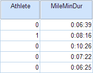
In the sample data, we will use two variables: Athlete and MileMinDur . The variable Athlete has values of either “0” (non-athlete) or "1" (athlete). It will function as the independent variable in this T test. The variable MileMinDur is a numeric duration variable (h:mm:ss), and it will function as the dependent variable. In SPSS, the first few rows of data look like this:
Before the Test
Before running the Independent Samples t Test, it is a good idea to look at descriptive statistics and graphs to get an idea of what to expect. Running Compare Means ( Analyze > Compare Means > Means ) to get descriptive statistics by group tells us that the standard deviation in mile time for non-athletes is about 2 minutes; for athletes, it is about 49 seconds. This corresponds to a variance of 14803 seconds for non-athletes, and a variance of 2447 seconds for athletes 1 . Running the Explore procedure ( Analyze > Descriptives > Explore ) to obtain a comparative boxplot yields the following graph:

If the variances were indeed equal, we would expect the total length of the boxplots to be about the same for both groups. However, from this boxplot, it is clear that the spread of observations for non-athletes is much greater than the spread of observations for athletes. Already, we can estimate that the variances for these two groups are quite different. It should not come as a surprise if we run the Independent Samples t Test and see that Levene's Test is significant.
Additionally, we should also decide on a significance level (typically denoted using the Greek letter alpha, α ) before we perform our hypothesis tests. The significance level is the threshold we use to decide whether a test result is significant. For this example, let's use α = 0.05.
1 When computing the variance of a duration variable (formatted as hh:mm:ss or mm:ss or mm:ss.s), SPSS converts the standard deviation value to seconds before squaring.
Running the Test
To run the Independent Samples t Test:
- Click Analyze > Compare Means > Independent-Samples T Test .
- Move the variable Athlete to the Grouping Variable field, and move the variable MileMinDur to the Test Variable(s) area. Now Athlete is defined as the independent variable and MileMinDur is defined as the dependent variable.
- Click Define Groups , which opens a new window. Use specified values is selected by default. Since our grouping variable is numerically coded (0 = "Non-athlete", 1 = "Athlete"), type “0” in the first text box, and “1” in the second text box. This indicates that we will compare groups 0 and 1, which correspond to non-athletes and athletes, respectively. Click Continue when finished.
- Click OK to run the Independent Samples t Test. Output for the analysis will display in the Output Viewer window.
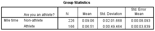
Two sections (boxes) appear in the output: Group Statistics and Independent Samples Test . The first section, Group Statistics , provides basic information about the group comparisons, including the sample size ( n ), mean, standard deviation, and standard error for mile times by group. In this example, there are 166 athletes and 226 non-athletes. The mean mile time for athletes is 6 minutes 51 seconds, and the mean mile time for non-athletes is 9 minutes 6 seconds.
The second section, Independent Samples Test , displays the results most relevant to the Independent Samples t Test. There are two parts that provide different pieces of information: (A) Levene’s Test for Equality of Variances and (B) t-test for Equality of Means.
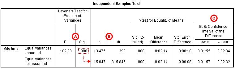
A Levene's Test for Equality of of Variances : This section has the test results for Levene's Test. From left to right:
- F is the test statistic of Levene's test
- Sig. is the p-value corresponding to this test statistic.
The p -value of Levene's test is printed as ".000" (but should be read as p < 0.001 -- i.e., p very small), so we we reject the null of Levene's test and conclude that the variance in mile time of athletes is significantly different than that of non-athletes. This tells us that we should look at the "Equal variances not assumed" row for the t test (and corresponding confidence interval) results . (If this test result had not been significant -- that is, if we had observed p > α -- then we would have used the "Equal variances assumed" output.)
B t-test for Equality of Means provides the results for the actual Independent Samples t Test. From left to right:
- t is the computed test statistic, using the formula for the equal-variances-assumed test statistic (first row of table) or the formula for the equal-variances-not-assumed test statistic (second row of table)
- df is the degrees of freedom, using the equal-variances-assumed degrees of freedom formula (first row of table) or the equal-variances-not-assumed degrees of freedom formula (second row of table)
- Sig (2-tailed) is the p-value corresponding to the given test statistic and degrees of freedom
- Mean Difference is the difference between the sample means, i.e. x 1 − x 2 ; it also corresponds to the numerator of the test statistic for that test
- Std. Error Difference is the standard error of the mean difference estimate; it also corresponds to the denominator of the test statistic for that test
Note that the mean difference is calculated by subtracting the mean of the second group from the mean of the first group. In this example, the mean mile time for athletes was subtracted from the mean mile time for non-athletes (9:06 minus 6:51 = 02:14). The sign of the mean difference corresponds to the sign of the t value. The positive t value in this example indicates that the mean mile time for the first group, non-athletes, is significantly greater than the mean for the second group, athletes.
The associated p value is printed as ".000"; double-clicking on the p-value will reveal the un-rounded number. SPSS rounds p-values to three decimal places, so any p-value too small to round up to .001 will print as .000. (In this particular example, the p-values are on the order of 10 -40 .)
C Confidence Interval of the Difference : This part of the t -test output complements the significance test results. Typically, if the CI for the mean difference contains 0 within the interval -- i.e., if the lower boundary of the CI is a negative number and the upper boundary of the CI is a positive number -- the results are not significant at the chosen significance level. In this example, the 95% CI is [01:57, 02:32], which does not contain zero; this agrees with the small p -value of the significance test.
Decision and Conclusions
Since p < .001 is less than our chosen significance level α = 0.05, we can reject the null hypothesis, and conclude that the that the mean mile time for athletes and non-athletes is significantly different.
Based on the results, we can state the following:
- There was a significant difference in mean mile time between non-athletes and athletes ( t 315.846 = 15.047, p < .001).
- The average mile time for athletes was 2 minutes and 14 seconds lower than the average mile time for non-athletes.
- << Previous: Paired Samples t Test
- Next: One-Way ANOVA >>
- Last Updated: Jun 14, 2024 11:54 AM
- URL: https://libguides.library.kent.edu/SPSS
Street Address
Mailing address, quick links.
- How Are We Doing?
- Student Jobs
Information
- Accessibility
- Emergency Information
- For Our Alumni
- For the Media
- Jobs & Employment
- Life at KSU
- Privacy Statement
- Technology Support
- Website Feedback
Runs Test SPSS
SPSS Tutorial (for Beginners): Intro to SPSS >
The runs test ((also called the Wald-Wolfowitz one-sample runs test) will tell you if the order of a binary variable is random or not. A “run” is a sequence of observations that change in a similar direction. For example, you might have a sequence of days when stock market values change in a positive direction (this is one run); this might be followed by a sequence of days when the stock market experiences negative price changes (this is a second run).
Although the runs test is based on binary sequences , it is usually applied to non-binary observations. SPSS will transform data into a binary sequence before calculating the results; the cut off point will be the median of the values unless you specify a cut off point (see Step 3 below).
According to IBM, the runs test can be performed quickly when your sample size is less than 30. Larger sample sizes may be very slow to compute [1].
Null Hypothesis for the Runs Test
Suppose you had a binary sequence with seven runs {1, 1, 0, 0, 0, 1, 0, 0, 0, 0, 1, 1, 1, 0, 0, 1, 1}.
The runs test tests the null hypothesis that the sequence of 1s and 0s was generated by N independent Bernoulli trials , each with probability p of generating a 1 and a probability 1 – p of generating a 0.
Runs Test SPSS: Steps
Step 1: Click Analyze, choose “Non Parametric Tests” and then “Legacy Dialogs”. Choose the Runs Test from the list.
Step 2: Move the variable you want to test over to the Test Variable box: click on the variable to highlight it, then click the blue center arrow to move the variable. Click “Options” and then place a check mark next to “Descriptive Statistics”.

Step 3: (Optional): If you want to specify your own cut off point, place a checkmark in the “Custom” box in the Cut Point section at the bottom of the Runs Test Window. This is where you will specify a cut point that separates your “ups” from “downs” (or highs to lows, or whatever else it is you are measuring.
If you don’t specify this, the Runs Test will use the default “median” of the scores for the cut-off to transform the data into a sequence of binary variables for the test. You can also choose to base the analysis of the mean or mode by checking that box. Usually, you would choose only one of these (mean, median, mode, or a specified cut point).
Step 4: Read the two-sided p-value for your result. If the p-value is small, this indicates a departure from randomness. For large p-values, the order is random.
Runs Test SPSS: References
[1] IBM SPSS Exact Tests . Retrieved February 18, 2022 from: http://bayes.acs.unt.edu:8083/BayesContent/class/Jon/SPSS_SC/Manuals/v19/IBM%20SPSS%20Exact%20Tests.pdf
EZ SPSS Tutorials
Calculate Sample Size for a Pearson Correlation in SPSS
In this tutorial, we show you how to calculate a minimum sample size for a Pearson correlation coefficient using SPSS power analysis. It is important to perform this calculation before you collect data for your study (although you may wish to carry out a pilot study beforehand).
Quick Steps
- Click Analyze -> Power Analysis -> Correlations -> Pearson Product Moment
- Click Reset (recommended)
- For Estimate , ensure that Sample size is selected
- In the Single power value box, enter your desired power value (typically .80 or higher)
- In the Pearson correlation parameter box, enter the expected correlation between your variables of interest
- In the Null value box, you will typically leave the value as 0
- Ensure that the Use bias-correction formula in the power estimate box is checked
- Under Test direction , select Nondirectional (two-sided) analysis or Directional (one-sided) analysis as applicable
- In the Significance level box, overtype the default value of 0.05 if applicable
- Click OK
What do we Need to Calculate Sample Size for a Pearson Correlation?
Imagine that we want to conduct a study to find out whether there is an association between the scores that students receive on their Spanish language exam and the number of minutes that they report studying for the exam. We plan to collect data from a sample of students, and then calculate a Pearson correlation coefficient to analyze this data. Before we collect any data, however, we want to estimate the minimum sample size that we need for our study.
To calculate the minimum sample size for a Pearson correlation test, we need the following:
- the power value
- the expected correlation between the variables of interest
- the correlation for the null hypothesis
- a decision about whether the alternative hypothesis is directional or non-directional
- the alpha level
Power Value
Power refers to the probability that a statistical test will detect an effect, difference, or correlation if that effect, difference, or correlation exists. If the test does not detect an effect when an effect does, in fact, exist, researchers will incorrectly fail to reject the null hypothesis, thereby committing a Type II error.
The standard convention is to use a power value of .80 (or higher). This means that we will detect a statistically significant effect 80% of the time if an effect exists.
In our example, this means that a Pearson correlation coefficient test will detect a significant correlation between students’ Spanish language exam scores and the number of minutes they report studying for the exam 80% of the time if these two variables are, in fact, correlated.
If all the other factors used to calculate sample size are held constant, the higher the power value, the larger the minimum sample size.
Expected Correlation Between the Variables of Interest
We need an estimate of the expected correlation between the two variables of interest. That is, we need to know the expected r value. You can base this estimate on: a pilot study; or one or more previous studies that are similar to yours.
If you can’t run a pilot study, and there are no previous studies that are similar to yours, however, you can use Cohen’s (1988) effect size recommendations to make an educated guess about the likely correlation coefficient between your variables: r = .10 (small effect), r = .30 (medium effect), and r = .50 (large effect)
For our example, we will use r = .34 based on the findings of a previous (fictitious) study that was similar to ours.
If all the other factors used to calculate sample size are held constant, the higher the expected correlation for the variables of interest, the smaller the minimum sample size.
Correlation for the Null Hypothesis
When we calculate a minimum sample size, we need to enter a correlation coefficient for our null hypothesis. For most studies, t he null hypothesis is that there is no correlation between the variables of interest (r = .00).
Directional or Non-Directional Alternative Hypothesis?
You will need to determine whether the alternative hypothesis for your study is directional (one-tailed) or non-directional (two-tailed). Since a previous study that was very similar to ours found a positive correlation between these two variables, we have opted for a directional hypothesis as follows:
- Students’ Spanish language exam scores are positively correlated with the number of minutes that they report studying for the exam (the more time they report studying for the exam, the higher their score).
If you cannot justify a directional hypothesis, you should use a non-directional hypothesis.
If all the other factors used to calculate sample size are held constant, you will need a larger sample size for a non-directional hypothesis than for a directional hypothesis.
Alpha Level
The alpha level (also known as the significance level or p value) refers to the probability that a statistical test will find an effect, difference, or correlation when, in fact, that effect, difference, or correlation does not exist. In other words, it is the probability that we will incorrectly reject the null hypothesis, thereby committing a Type I error.
The standard convention is to set the alpha level at .05 (or less), which means that there is a 5% probability that we will reject the null hypothesis when, in fact, that effect, difference, or correlation does not exist.
If all the other factors used to calculate sample size are held constant, the lower the alpha level, the larger the minimum sample size.
Calculating Sample Size for a Pearson Correlation Using SPSS Power Analysis
To calculate a sample size for a Pearson Correlation, first click Analyze -> Power Analysis -> Correlations -> Pearson Product Moment

This brings up the Power Analysis: Pearson Correlation dialog box .
We recommend clicking the Reset button to clear any previous settings.

Under Test Assumptions , for Estimate , ensure that Sample size is selected.
Then, in the Single power value box, enter your desired power value. For our example, we will enter .80 following the standard convention.
In the Pearson correlation parameter box, enter the expected correlation between your variables of interest. We enter a value of .34 on the basis of a previous (fictitious) study that was similar to ours.
In the Null value box, we leave the default value of 0 unchanged. We rarely need to change this.
Ensure that the Use-bias correction formula in the power estimate box is checked.
Under Test direction , the Nondirectional (two-sided) analysis option is selected by default. You should only select the Directional (one-sided) analysis option if you can justify this decision. In our example, we select the the Directional (one-sided) analysis option on the basis of the results of a previous similar (fictitious) study.
By default, the Significance level box is set to a value of 0.05. if you intend to use an alpha level other than .05, overtype this value with your chosen alpha level.
The screenshot below shows the Power Analysis: Pearson Correlation dialog box populated with our example values:

The Minimum Sample Size
The SPSS Output Viewer will pop up with the results of your minimum sample size calculation. As you can see, the minimum sample size for our example Pearson correlation test is 52. If you don’t think that the minimum sample size calculated for your study is feasible, consider running the calculation again with different values.

***************
That’s it for this tutorial. You should now be able to calculate the minimum sample size for a Pearson correlation coefficient using SPSS power analysis.

Snapsolve any problem by taking a picture. Try it in the Numerade app?
IMAGES
VIDEO
COMMENTS
By Ruben Geert van den Berg under Statistics A-Z. A null hypothesis is a precise statement about a population that we try to reject with sample data. We don't usually believe our null hypothesis (or H 0) to be true. However, we need some exact statement as a starting point for statistical significance testing.
This section and the "Graphics" section provide a quick tutorial for a few common functions in SPSS, primarily to provide the reader with a feel for the SPSS user interface. This is not a comprehensive tutorial, but SPSS itself provides comprehensive tutorials and case studies through it's help menu. SPSS's help menu is more than a quick reference.
This video demonstrates how to test the null hypothesis with ANOVA in SPSS. In the case of ANOVA, the null hypothesis states the mean score for each group is...
We cannot change the null hypothesis of a t test in SPSS, but we can use the confidence interval to test this null hypothesis as explained in Section 4.6.1. In SPSS, the analyst has to specify the null hypothesis in tests on one variable, namely tests on one proportion, one mean, or one categorical variable.
Created by the ITS Training Program at CSULA for students. Hypothesis Testing: SPSS (2.1): The null hypothesis (H0) represents a theory that has been presented, either because it is believed to be true or because it is to be used as a basis for an argument. It is a statement that has not been proven. It is also important to realize that t….
Review. In a hypothesis test, sample data is evaluated in order to arrive at a decision about some type of claim.If certain conditions about the sample are satisfied, then the claim can be evaluated for a population. In a hypothesis test, we: Evaluate the null hypothesis, typically denoted with \(H_{0}\).The null is not rejected unless the hypothesis test shows otherwise.
In SPSS we can load that file and then run the following procedure: Once in the appropriate dialog, you would select Success as your variable (it's the only one) and then select Exact Binomial as the test type: Click on OK and you'll get something like this: Right now, this output looks pretty unfamiliar to you, but you can see that it's ...
SPSS & Hypothesis Testing. Hypothesis testing is a decision making process for evaluating claims about a population. Q1: Give at least three examples of a population. Q2: For the population listed in 1), give an example of a sample from the population. Q3: Can you make up some hypothesis about the population in 1).
The actual test begins by considering two hypotheses.They are called the null hypothesis and the alternative hypothesis.These hypotheses contain opposing viewpoints. H 0, the —null hypothesis: a statement of no difference between sample means or proportions or no difference between a sample mean or proportion and a population mean or proportion. In other words, the difference equals 0.
A null hypothesis does not make a resolute claim of no relationship. But, rather, says there's a lack of proof. That, we cannot statistically measure a significant relationship between the variables.
Null hypothesis (H 0): Independent variable does not affect dependent variable. Alternative hypothesis (H a): Independent variable affects dependent variable. Test-specific template sentences. Once you know the statistical test you'll be using, you can write your hypotheses in a more precise and mathematical way specific to the test you chose ...
H 0 (Null Hypothesis): Population parameter =, ≤, ≥ some value. H A (Alternative Hypothesis): Population parameter <, >, ≠ some value. Note that the null hypothesis always contains the equal sign. We interpret the hypotheses as follows: Null hypothesis: The sample data provides no evidence to support some claim being made by an individual.
8.5: The p value of a Test. In one sense, our hypothesis test is complete; we've constructed a test statistic, figured out its sampling distribution if the null hypothesis is true, and then constructed the critical region for the test. Nevertheless, we've actually omitted the most important number of all: the p value.
Statistical significance is the probability of finding a given deviation from the null hypothesis -or a more extreme one- in a sample. Statistical significance is often referred to as the p-value (short for "probability value") or simply p in research papers. A small p-value basically means that your data are unlikely under some null ...
The significance for this test SPSS calculated as 0.608 which is quite high and consequently the recommendation is to retain the null hypothesis (as the significance level is 0.05), which in this case means that the proportions male and female are about equal. Written by Johan Osterberg who lives and works in Gothenburg, Sweden as a developer ...
The null hypothesis (H 0) and (two-tailed) alternative hypothesis ... To run a One Sample t Test in SPSS, click Analyze > Compare Means > One-Sample T Test. The One-Sample T Test window opens where you will specify the variables to be used in the analysis. All of the variables in your dataset appear in the list on the left side.
Let's return finally to the question of whether we reject or fail to reject the null hypothesis. If our statistical analysis shows that the significance level is below the cut-off value we have set (e.g., either 0.05 or 0.01), we reject the null hypothesis and accept the alternative hypothesis. Alternatively, if the significance level is above ...
The null hypothesis (H 0) and alternative hypothesis (H 1) of the Independent Samples t Test can be expressed in two different but equivalent ways:H 0: µ 1 = µ 2 ("the two population means are equal") H 1: µ 1 ≠ µ 2 ("the two population means are not equal"). OR. H 0: µ 1 - µ 2 = 0 ("the difference between the two population means is equal to 0") H 1: µ 1 - µ 2 ≠ 0 ("the difference ...
The general procedure for testing the null hypothesis is as follows: State the null and alternative hypotheses. Specify α and the sample size. Select an appropriate statistical test. Collect data (note that the previous steps should be done before collecting data) Compute the test statistic based on the sample data.
Runs Test SPSS: Steps. Step 1: Click Analyze, choose "Non Parametric Tests" and then "Legacy Dialogs". Choose the Runs Test from the list. Step 2: Move the variable you want to test over to the Test Variable box: click on the variable to highlight it, then click the blue center arrow to move the variable. Click "Options" and then ...
To perform a Chi-Square test of Independence, click the Analyze tab, then click Descriptive Statistics, then click Crosstabs: In the new window that appears, drag Gender into the Rows panel, then drag Party into the Columns panel: Next, click the Cells button. Then check the boxes next to Observed and Expected: Then click Continue.
To calculate a sample size for a Pearson Correlation, first click Analyze -> Power Analysis -> Correlations -> Pearson Product Moment. This brings up the Power Analysis: Pearson Correlation dialog box. We recommend clicking the Reset button to clear any previous settings. Under Test Assumptions, for Estimate, ensure that Sample size is selected.
Then click the Plots button. Check the box next to Histogram and Normality plots with tests: Then click Continue. Then click OK. The following output will be generated that shows the results of the Shapiro-Wilk test along with a histogram that displays the distribution of exam scores: From the output we can see that the p-value of the Shapiro ...
Specifically, the four steps involved in using the critical value approach to conducting any hypothesis test are: Specify the null and alternative hypotheses. Using the sample data and assuming the null hypothesis is true, calculate the value of the test statistic.
Calculate the t-statistic using the computer program SPSS, include effect size Write the t-statistic using proper APA format Decide whether or not you would reject the null hypothesis Interpret this result Independent Sample T-Test: A researcher is interested in the difference in rural and urban people's attitudes towards gun control.