hypothesis on regression

Statistics Made Easy

Understanding the Null Hypothesis for Linear Regression

Linear regression is a technique we can use to understand the relationship between one or more predictor variables and a response variable .

If we only have one predictor variable and one response variable, we can use simple linear regression , which uses the following formula to estimate the relationship between the variables:

ŷ = β 0 + β 1 x

ŷ: The estimated response value.
β 0 : The average value of y when x is zero.
β 1 : The average change in y associated with a one unit increase in x.
x: The value of the predictor variable.

Simple linear regression uses the following null and alternative hypotheses:

H 0 : β 1 = 0
H A : β 1 ≠ 0

The null hypothesis states that the coefficient β 1 is equal to zero. In other words, there is no statistically significant relationship between the predictor variable, x, and the response variable, y.

The alternative hypothesis states that β 1 is not equal to zero. In other words, there is a statistically significant relationship between x and y.

If we have multiple predictor variables and one response variable, we can use multiple linear regression , which uses the following formula to estimate the relationship between the variables:

ŷ = β 0 + β 1 x 1 + β 2 x 2 + … + β k x k

β 0 : The average value of y when all predictor variables are equal to zero.
β i : The average change in y associated with a one unit increase in x i .
x i : The value of the predictor variable x i .

Multiple linear regression uses the following null and alternative hypotheses:

H 0 : β 1 = β 2 = … = β k = 0
H A : β 1 = β 2 = … = β k ≠ 0

The null hypothesis states that all coefficients in the model are equal to zero. In other words, none of the predictor variables have a statistically significant relationship with the response variable, y.

The alternative hypothesis states that not every coefficient is simultaneously equal to zero.

The following examples show how to decide to reject or fail to reject the null hypothesis in both simple linear regression and multiple linear regression models.

Example 1: Simple Linear Regression

Suppose a professor would like to use the number of hours studied to predict the exam score that students will receive in his class. He collects data for 20 students and fits a simple linear regression model.

The following screenshot shows the output of the regression model:

Output of simple linear regression in Excel

The fitted simple linear regression model is:

Exam Score = 67.1617 + 5.2503*(hours studied)

To determine if there is a statistically significant relationship between hours studied and exam score, we need to analyze the overall F value of the model and the corresponding p-value:

Overall F-Value: 47.9952
P-value: 0.000

Since this p-value is less than .05, we can reject the null hypothesis. In other words, there is a statistically significant relationship between hours studied and exam score received.

Example 2: Multiple Linear Regression

Suppose a professor would like to use the number of hours studied and the number of prep exams taken to predict the exam score that students will receive in his class. He collects data for 20 students and fits a multiple linear regression model.

Multiple linear regression output in Excel

The fitted multiple linear regression model is:

Exam Score = 67.67 + 5.56*(hours studied) – 0.60*(prep exams taken)

To determine if there is a jointly statistically significant relationship between the two predictor variables and the response variable, we need to analyze the overall F value of the model and the corresponding p-value:

Overall F-Value: 23.46
P-value: 0.00

Since this p-value is less than .05, we can reject the null hypothesis. In other words, hours studied and prep exams taken have a jointly statistically significant relationship with exam score.

Note: Although the p-value for prep exams taken (p = 0.52) is not significant, prep exams combined with hours studied has a significant relationship with exam score.

Additional Resources

Understanding the F-Test of Overall Significance in Regression How to Read and Interpret a Regression Table How to Report Regression Results How to Perform Simple Linear Regression in Excel How to Perform Multiple Linear Regression in Excel

Featured Posts

5 Regularization Techniques You Should Know

Hey there. My name is Zach Bobbitt. I have a Masters of Science degree in Applied Statistics and I’ve worked on machine learning algorithms for professional businesses in both healthcare and retail. I’m passionate about statistics, machine learning, and data visualization and I created Statology to be a resource for both students and teachers alike. My goal with this site is to help you learn statistics through using simple terms, plenty of real-world examples, and helpful illustrations.

2 Replies to “Understanding the Null Hypothesis for Linear Regression”

Thank you Zach, this helped me on homework!

Great articles, Zach.

I would like to cite your work in a research paper.

Could you provide me with your last name and initials.

Join the Statology Community

Sign up to receive Statology's exclusive study resource: 100 practice problems with step-by-step solutions. Plus, get our latest insights, tutorials, and data analysis tips straight to your inbox!

By subscribing you accept Statology's Privacy Policy.

Want to create or adapt books like this? Learn more about how Pressbooks supports open publishing practices.

13.6 Testing the Regression Coefficients

Learning objectives.

Conduct and interpret a hypothesis test on individual regression coefficients.

Previously, we learned that the population model for the multiple regression equation is

[latex]\begin{eqnarray*} y & = & \beta_0+\beta_1x_1+\beta_2x_2+\cdots+\beta_kx_k +\epsilon \end{eqnarray*}[/latex]

where [latex]x_1,x_2,\ldots,x_k[/latex] are the independent variables, [latex]\beta_0,\beta_1,\ldots,\beta_k[/latex] are the population parameters of the regression coefficients, and [latex]\epsilon[/latex] is the error variable. In multiple regression, we estimate each population regression coefficient [latex]\beta_i[/latex] with the sample regression coefficient [latex]b_i[/latex].

In the previous section, we learned how to conduct an overall model test to determine if the regression model is valid. If the outcome of the overall model test is that the model is valid, then at least one of the independent variables is related to the dependent variable—in other words, at least one of the regression coefficients [latex]\beta_i[/latex] is not zero. However, the overall model test does not tell us which independent variables are related to the dependent variable. To determine which independent variables are related to the dependent variable, we must test each of the regression coefficients.

Testing the Regression Coefficients

For an individual regression coefficient, we want to test if there is a relationship between the dependent variable [latex]y[/latex] and the independent variable [latex]x_i[/latex].

No Relationship . There is no relationship between the dependent variable [latex]y[/latex] and the independent variable [latex]x_i[/latex]. In this case, the regression coefficient [latex]\beta_i[/latex] is zero. This is the claim for the null hypothesis in an individual regression coefficient test: [latex]H_0: \beta_i=0[/latex].
Relationship. There is a relationship between the dependent variable [latex]y[/latex] and the independent variable [latex]x_i[/latex]. In this case, the regression coefficients [latex]\beta_i[/latex] is not zero. This is the claim for the alternative hypothesis in an individual regression coefficient test: [latex]H_a: \beta_i \neq 0[/latex]. We are not interested if the regression coefficient [latex]\beta_i[/latex] is positive or negative, only that it is not zero. We only need to find out if the regression coefficient is not zero to demonstrate that there is a relationship between the dependent variable and the independent variable. This makes the test on a regression coefficient a two-tailed test.

In order to conduct a hypothesis test on an individual regression coefficient [latex]\beta_i[/latex], we need to use the distribution of the sample regression coefficient [latex]b_i[/latex]:

The mean of the distribution of the sample regression coefficient is the population regression coefficient [latex]\beta_i[/latex].
The standard deviation of the distribution of the sample regression coefficient is [latex]\sigma_{b_i}[/latex]. Because we do not know the population standard deviation we must estimate [latex]\sigma_{b_i}[/latex] with the sample standard deviation [latex]s_{b_i}[/latex].
The distribution of the sample regression coefficient follows a normal distribution.

Steps to Conduct a Hypothesis Test on a Regression Coefficient

[latex]\begin{eqnarray*} H_0: & & \beta_i=0 \\ \\ \end{eqnarray*}[/latex]

[latex]\begin{eqnarray*} H_a: & & \beta_i \neq 0 \\ \\ \end{eqnarray*}[/latex]

Collect the sample information for the test and identify the significance level [latex]\alpha[/latex].

[latex]\begin{eqnarray*}t & = & \frac{b_i-\beta_i}{s_{b_i}} \\ \\ df & = & n-k-1 \\ \\ \end{eqnarray*}[/latex]

The results of the sample data are significant. There is sufficient evidence to conclude that the null hypothesis [latex]H_0[/latex] is an incorrect belief and that the alternative hypothesis [latex]H_a[/latex] is most likely correct.
The results of the sample data are not significant. There is not sufficient evidence to conclude that the alternative hypothesis [latex]H_a[/latex] may be correct.
Write down a concluding sentence specific to the context of the question.

The required [latex]t[/latex]-score and p -value for the test can be found on the regression summary table, which we learned how to generate in Excel in a previous section.

The human resources department at a large company wants to develop a model to predict an employee’s job satisfaction from the number of hours of unpaid work per week the employee does, the employee’s age, and the employee’s income. A sample of 25 employees at the company is taken and the data is recorded in the table below. The employee’s income is recorded in $1000s and the job satisfaction score is out of 10, with higher values indicating greater job satisfaction.

Previously, we found the multiple regression equation to predict the job satisfaction score from the other variables:

[latex]\begin{eqnarray*} \hat{y} & = & 4.7993-0.3818x_1+0.0046x_2+0.0233x_3 \\ \\ \hat{y} & = & \mbox{predicted job satisfaction score} \\ x_1 & = & \mbox{hours of unpaid work per week} \\ x_2 & = & \mbox{age} \\ x_3 & = & \mbox{income (\$1000s)}\end{eqnarray*}[/latex]

At the 5% significance level, test the relationship between the dependent variable “job satisfaction” and the independent variable “hours of unpaid work per week”.

Hypotheses:

[latex]\begin{eqnarray*} H_0: & & \beta_1=0 \\ H_a: & & \beta_1 \neq 0 \end{eqnarray*}[/latex]

The regression summary table generated by Excel is shown below:

The p -value for the test on the hours of unpaid work per week regression coefficient is in the bottom part of the table under the P-value column of the Hours of Unpaid Work per Week row . So the p -value=[latex]0.0082[/latex].

Conclusion:

Because p -value[latex]=0.0082 \lt 0.05=\alpha[/latex], we reject the null hypothesis in favour of the alternative hypothesis. At the 5% significance level there is enough evidence to suggest that there is a relationship between the dependent variable “job satisfaction” and the independent variable “hours of unpaid work per week.”

The null hypothesis [latex]\beta_1=0[/latex] is the claim that the regression coefficient for the independent variable [latex]x_1[/latex] is zero. That is, the null hypothesis is the claim that there is no relationship between the dependent variable and the independent variable “hours of unpaid work per week.”
The alternative hypothesis is the claim that the regression coefficient for the independent variable [latex]x_1[/latex] is not zero. The alternative hypothesis is the claim that there is a relationship between the dependent variable and the independent variable “hours of unpaid work per week.”
When conducting a test on a regression coefficient, make sure to use the correct subscript on [latex]\beta[/latex] to correspond to how the independent variables were defined in the regression model and which independent variable is being tested. Here the subscript on [latex]\beta[/latex] is 1 because the “hours of unpaid work per week” is defined as [latex]x_1[/latex] in the regression model.
The p -value for the tests on the regression coefficients are located in the bottom part of the table under the P-value column heading in the corresponding independent variable row.
Because the alternative hypothesis is a [latex]\neq[/latex], the p -value is the sum of the area in the tails of the [latex]t[/latex]-distribution. This is the value calculated out by Excel in the regression summary table.
The p -value of 0.0082 is a small probability compared to the significance level, and so is unlikely to happen assuming the null hypothesis is true. This suggests that the assumption that the null hypothesis is true is most likely incorrect, and so the conclusion of the test is to reject the null hypothesis in favour of the alternative hypothesis. In other words, the regression coefficient [latex]\beta_1[/latex] is not zero, and so there is a relationship between the dependent variable “job satisfaction” and the independent variable “hours of unpaid work per week.” This means that the independent variable “hours of unpaid work per week” is useful in predicting the dependent variable.

At the 5% significance level, test the relationship between the dependent variable “job satisfaction” and the independent variable “age”.

[latex]\begin{eqnarray*} H_0: & & \beta_2=0 \\ H_a: & & \beta_2 \neq 0 \end{eqnarray*}[/latex]

The p -value for the test on the age regression coefficient is in the bottom part of the table under the P-value column of the Age row . So the p -value=[latex]0.8439[/latex].

Because p -value[latex]=0.8439 \gt 0.05=\alpha[/latex], we do not reject the null hypothesis. At the 5% significance level there is not enough evidence to suggest that there is a relationship between the dependent variable “job satisfaction” and the independent variable “age.”

The null hypothesis [latex]\beta_2=0[/latex] is the claim that the regression coefficient for the independent variable [latex]x_2[/latex] is zero. That is, the null hypothesis is the claim that there is no relationship between the dependent variable and the independent variable “age.”
The alternative hypothesis is the claim that the regression coefficient for the independent variable [latex]x_2[/latex] is not zero. The alternative hypothesis is the claim that there is a relationship between the dependent variable and the independent variable “age.”
When conducting a test on a regression coefficient, make sure to use the correct subscript on [latex]\beta[/latex] to correspond to how the independent variables were defined in the regression model and which independent variable is being tested. Here the subscript on [latex]\beta[/latex] is 2 because “age” is defined as [latex]x_2[/latex] in the regression model.
The p -value of 0.8439 is a large probability compared to the significance level, and so is likely to happen assuming the null hypothesis is true. This suggests that the assumption that the null hypothesis is true is most likely correct, and so the conclusion of the test is to not reject the null hypothesis. In other words, the regression coefficient [latex]\beta_2[/latex] is zero, and so there is no relationship between the dependent variable “job satisfaction” and the independent variable “age.” This means that the independent variable “age” is not particularly useful in predicting the dependent variable.

At the 5% significance level, test the relationship between the dependent variable “job satisfaction” and the independent variable “income”.

[latex]\begin{eqnarray*} H_0: & & \beta_3=0 \\ H_a: & & \beta_3 \neq 0 \end{eqnarray*}[/latex]

The p -value for the test on the income regression coefficient is in the bottom part of the table under the P-value column of the Income row . So the p -value=[latex]0.0060[/latex].

Because p -value[latex]=0.0060 \lt 0.05=\alpha[/latex], we reject the null hypothesis in favour of the alternative hypothesis. At the 5% significance level there is enough evidence to suggest that there is a relationship between the dependent variable “job satisfaction” and the independent variable “income.”

The null hypothesis [latex]\beta_3=0[/latex] is the claim that the regression coefficient for the independent variable [latex]x_3[/latex] is zero. That is, the null hypothesis is the claim that there is no relationship between the dependent variable and the independent variable “income.”
The alternative hypothesis is the claim that the regression coefficient for the independent variable [latex]x_3[/latex] is not zero. The alternative hypothesis is the claim that there is a relationship between the dependent variable and the independent variable “income.”
When conducting a test on a regression coefficient, make sure to use the correct subscript on [latex]\beta[/latex] to correspond to how the independent variables were defined in the regression model and which independent variable is being tested. Here the subscript on [latex]\beta[/latex] is 3 because “income” is defined as [latex]x_3[/latex] in the regression model.
The p -value of 0.0060 is a small probability compared to the significance level, and so is unlikely to happen assuming the null hypothesis is true. This suggests that the assumption that the null hypothesis is true is most likely incorrect, and so the conclusion of the test is to reject the null hypothesis in favour of the alternative hypothesis. In other words, the regression coefficient [latex]\beta_3[/latex] is not zero, and so there is a relationship between the dependent variable “job satisfaction” and the independent variable “income.” This means that the independent variable “income” is useful in predicting the dependent variable.

Concept Review

The test on a regression coefficient determines if there is a relationship between the dependent variable and the corresponding independent variable. The p -value for the test is the sum of the area in tails of the [latex]t[/latex]-distribution. The p -value can be found on the regression summary table generated by Excel.

The hypothesis test for a regression coefficient is a well established process:

Write down the null and alternative hypotheses in terms of the regression coefficient being tested. The null hypothesis is the claim that there is no relationship between the dependent variable and independent variable. The alternative hypothesis is the claim that there is a relationship between the dependent variable and independent variable.
Collect the sample information for the test and identify the significance level.
The p -value is the sum of the area in the tails of the [latex]t[/latex]-distribution. Use the regression summary table generated by Excel to find the p -value.
Compare the p -value to the significance level and state the outcome of the test.

Save 10% on All AnalystPrep 2024 Study Packages with Coupon Code BLOG10 .

Payment Plans
Product List
Partnerships

Try Free Trial
Study Packages
Levels I, II & III Lifetime Package
Video Lessons
Study Notes
Practice Questions
Levels II & III Lifetime Package
About the Exam
About your Instructor
Part I Study Packages
Part I & Part II Lifetime Package
Part II Study Packages
Exams P & FM Lifetime Package
Quantitative Questions
Verbal Questions
Data Insight Questions
Live Tutoring
About your Instructors
EA Practice Questions
Data Sufficiency Questions
Integrated Reasoning Questions

Hypothesis Testing in Regression Analysis

Hypothesis testing is used to confirm if the estimated regression coefficients bear any statistical significance. Either the confidence interval approach or the t-test approach can be used in hypothesis testing. In this section, we will explore the t-test approach.

The t-test Approach

The following are the steps followed in the performance of the t-test:

Set the significance level for the test.
Formulate the null and the alternative hypotheses.

$$t=\frac{\widehat{b_1}-b_1}{s_{\widehat{b_1}}}$$

$b_1$ = True slope coefficient.

$\widehat{b_1}$ = Point estimate for $b_1$

$b_1 s_{\widehat{b_1\ }}$ = Standard error of the regression coefficient.

Compare the absolute value of the t-statistic to the critical t-value (t_c). Reject the null hypothesis if the absolute value of the t-statistic is greater than the critical t-value i.e., $t\ >\ +\ t_{critical}\ or\ t\ <\ –t_{\text{critical}}$.

Example: Hypothesis Testing of the Significance of Regression Coefficients

An analyst generates the following output from the regression analysis of inflation on unemployment:

$$\small{\begin{array}{llll}\hline{}& \textbf{Regression Statistics} &{}&{}\\ \hline{}& \text{Multiple R} & 0.8766 &{} \\ {}& \text{R Square} & 0.7684 &{} \\ {}& \text{Adjusted R Square} & 0.7394 & {}\\ {}& \text{Standard Error} & 0.0063 &{}\\ {}& \text{Observations} & 10 &{}\\ \hline {}& & & \\ \hline{} & \textbf{Coefficients} & \textbf{Standard Error} & \textbf{t-Stat}\\ \hline \text{Intercept} & 0.0710 & 0.0094 & 7.5160 \\\text{Forecast (Slope)} & -0.9041 & 0.1755 & -5.1516\\ \hline\end{array}}$$

At the 5% significant level, test the null hypothesis that the slope coefficient is significantly different from one, that is,

$$ H_{0}: b_{1} = 1\ vs. \ H_{a}: b_{1}≠1 $$

The calculated t-statistic, $\text{t}=\frac{\widehat{b_{1}}-b_1}{\widehat{S_{b_{1}}}}$ is equal to:

$$\begin{align*}\text{t}& = \frac{-0.9041-1}{0.1755}\\& = -10.85\end{align*}$$

The critical two-tail t-values from the table with $n-2=8$ degrees of freedom are:

$$\text{t}_{c}=±2.306$$

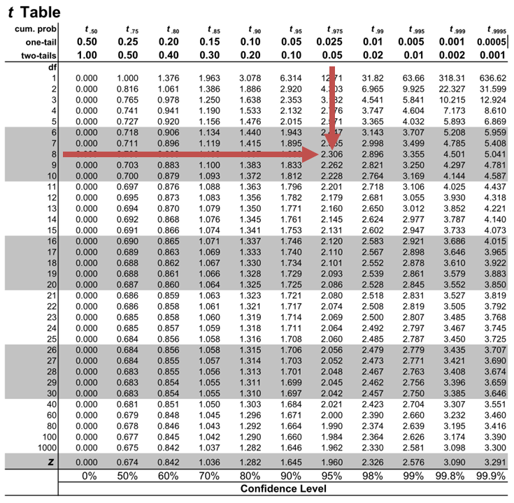
Notice that $|t|>t_{c}$ i.e., ($10.85>2.306$)

Therefore, we reject the null hypothesis and conclude that the estimated slope coefficient is statistically different from one.

Note that we used the confidence interval approach and arrived at the same conclusion.

Question Neeth Shinu, CFA, is forecasting price elasticity of supply for a certain product. Shinu uses the quantity of the product supplied for the past 5months as the dependent variable and the price per unit of the product as the independent variable. The regression results are shown below. $$\small{\begin{array}{lccccc}\hline \textbf{Regression Statistics} & & & & & \\ \hline \text{Multiple R} & 0.9971 & {}& {}&{}\\ \text{R Square} & 0.9941 & & & \\ \text{Adjusted R Square} & 0.9922 & & & & \\ \text{Standard Error} & 3.6515 & & & \\ \text{Observations} & 5 & & & \\ \hline {}& \textbf{Coefficients} & \textbf{Standard Error} & \textbf{t Stat} & \textbf{P-value}\\ \hline\text{Intercept} & -159 & 10.520 & (15.114) & 0.001\\ \text{Slope} & 0.26 & 0.012 & 22.517 & 0.000\\ \hline\end{array}}$$ Which of the following most likely reports the correct value of the t-statistic for the slope and most accurately evaluates its statistical significance with 95% confidence? A. $t=21.67$; slope is significantly different from zero. B. $t= 3.18$; slope is significantly different from zero. C. $t=22.57$; slope is not significantly different from zero. Solution The correct answer is A . The t-statistic is calculated using the formula: $$\text{t}=\frac{\widehat{b_{1}}-b_1}{\widehat{S_{b_{1}}}}$$ Where: $b_{1}$ = True slope coefficient $\widehat{b_{1}}$ = Point estimator for $b_{1}$ $\widehat{S_{b_{1}}}$ = Standard error of the regression coefficient $$\begin{align*}\text{t}&=\frac{0.26-0}{0.012}\\&=21.67\end{align*}$$ The critical two-tail t-values from the t-table with $n-2 = 3$ degrees of freedom are: $$t_{c}=±3.18$$ Notice that $|t|>t_{c}$ (i.e $21.67>3.18$). Therefore, the null hypothesis can be rejected. Further, we can conclude that the estimated slope coefficient is statistically different from zero.

Offered by AnalystPrep

Analysis of Variance (ANOVA)

Predicted value of a dependent variable, uses of the t-test and the z-test.

The z-test The z-test is the ideal hypothesis test to conduct in a... Read More

Solving Counting Problems through Labe ...

Counting problems involve determination of the exact number of ways two or more... Read More

Continuous Uniform Distribution

The continuous uniform distribution is such that the random variable X takes values... Read More

Parametric and Non-Parametric Test

Parametric versus Non-parametric Tests of Independence A parametric test is a hypothesis test... Read More

Linear regression - Hypothesis testing

by Marco Taboga , PhD

This lecture discusses how to perform tests of hypotheses about the coefficients of a linear regression model estimated by ordinary least squares (OLS).

Table of contents

Normal vs non-normal model

The linear regression model, matrix notation, tests of hypothesis in the normal linear regression model, test of a restriction on a single coefficient (t test), test of a set of linear restrictions (f test), tests based on maximum likelihood procedures (wald, lagrange multiplier, likelihood ratio), tests of hypothesis when the ols estimator is asymptotically normal, test of a restriction on a single coefficient (z test), test of a set of linear restrictions (chi-square test), learn more about regression analysis.

The lecture is divided in two parts:

in the first part, we discuss hypothesis testing in the normal linear regression model , in which the OLS estimator of the coefficients has a normal distribution conditional on the matrix of regressors;

in the second part, we show how to carry out hypothesis tests in linear regression analyses where the hypothesis of normality holds only in large samples (i.e., the OLS estimator can be proved to be asymptotically normal).

How to choose which test to carry out after estimating a linear regression model.

We also denote:

We now explain how to derive tests about the coefficients of the normal linear regression model.

It can be proved (see the lecture about the normal linear regression model ) that the assumption of conditional normality implies that:

How the acceptance region is determined depends not only on the desired size of the test , but also on whether the test is:

one-tailed (only one of the two things, i.e., either smaller or larger, is possible).

For more details on how to determine the acceptance region, see the glossary entry on critical values .

The F test is one-tailed .

A critical value in the right tail of the F distribution is chosen so as to achieve the desired size of the test.

Then, the null hypothesis is rejected if the F statistics is larger than the critical value.

In this section we explain how to perform hypothesis tests about the coefficients of a linear regression model when the OLS estimator is asymptotically normal.

As we have shown in the lecture on the properties of the OLS estimator , in several cases (i.e., under different sets of assumptions) it can be proved that:

These two properties are used to derive the asymptotic distribution of the test statistics used in hypothesis testing.

The test can be either one-tailed or two-tailed . The same comments made for the t-test apply here.

Like the F test, also the Chi-square test is usually one-tailed .

The desired size of the test is achieved by appropriately choosing a critical value in the right tail of the Chi-square distribution.

The null is rejected if the Chi-square statistics is larger than the critical value.

Want to learn more about regression analysis? Here are some suggestions:

R squared of a linear regression ;

Gauss-Markov theorem ;

Generalized Least Squares ;

Multicollinearity ;

Dummy variables ;

Selection of linear regression models

Partitioned regression ;

Ridge regression .

How to cite

Please cite as:

Taboga, Marco (2021). "Linear regression - Hypothesis testing", Lectures on probability theory and mathematical statistics. Kindle Direct Publishing. Online appendix. https://www.statlect.com/fundamentals-of-statistics/linear-regression-hypothesis-testing.

Most of the learning materials found on this website are now available in a traditional textbook format.

F distribution
Beta distribution
Conditional probability
Central Limit Theorem
Binomial distribution
Mean square convergence
Delta method
Almost sure convergence
Mathematical tools
Fundamentals of probability
Probability distributions
Asymptotic theory
Fundamentals of statistics
About Statlect
Cookies, privacy and terms of use
Loss function
Almost sure
Type I error
Precision matrix
Integrable variable
To enhance your privacy,
we removed the social buttons,
but don't forget to share .

H 0 : β = 0 (Null hypothesis)
H A : β ≠ 0 (Alternative hypothesis)

Part of Dr. Doug Elrod 's A (Brief) Theory of Regression Talk

Remember the regression equation for predicting y from x is: y = bx + a (a is also indicated as "e" at times)

b , or the slope, is simply (r xy * S.D. y )/S.D. x a , or the intercept, is simply the value of y when x is 0:

[Why?: the point, a, where the line crosses the Y axis for X being 0 is the distance from the mean of Y predicted for the X value of 0: Remember: D y = b * D x a = D y + mean of y so:

] Example: Let's say we knew that the average UCLA student experiences a moderate level of anxiety on a 100 point scale, = 36.8, S.D. = 12.2. Also, that students average a course load of about 13 or so units, = 13.4, S.D. = 3.7. And finally, that the correlation between units taken and anxiety levels is a stunning r = .4. You might ask as you plan your schedule for next quarter, how much anxiety can I expect to experience if I take 20 units? Treat units as x and anxiety as y. Then The slope of the line predicting anxiety from units taken is (.4 * 12.2)/3.7 = (4.88)/3.7 = 1.32 The intercept is 36.8 - 1.32*13.4 = 36.8 - 17.67 = 19.13 So the predicted anxiety score when taking 20 units is: y (or anxiety) = 1.32 * (20 units) + 19.13 = 45.53

The method of least squares

The r.m.s. error for the regression line of y on x is:

The regression equation is the equation for the line that produces the least r.m.s. error or standard error of the estimate If x and y are perfectly related, that is all points lie on the regression line, the standard error of estimate is zero (the square root of 1 - 1 2 = 0), there is no deviation from the line. If x and y are not associated at all, the standard error of the estimate is the S.D. of y (the square root of 1 - 0 2 = 1) and slope is 0. So the regression line is simply a line parallel to the x axis that intercepts y at the mean of y.

Interpretation

Regression is appropriate when the relationship between two variables is linear Although we commonly think of x as causing y, this is dependent upon the research design and logic GIGO--garbage in-garbage out--you can always create regression lines predicting one variable from another. The math is the same whether or not the analysis is appropriate

Example: Calculate a regression line predicting height of the surf at Venice beach from the number of floors in the math building.

So far we have learned how to take raw data, combine it, and create statistics that allow us to describe the data in a brief summary form.

We have used statistics to describe our samples. These are called descriptive statistics. We have used our statistics to say something about the population that our samples were drawn from--this is inferential statistics. Now we are going to learn another way in which statistics can be use inferentially--hypothesis testing

At the beginning of this course, we said that an important aspect of doing research is to specify our research question

The first step in conducting research is to translate our inclinations, hunches, suspicions, beliefs into a precise question.

Example: Is this drug effective?, Does lowering the interest rate cause inflation?

The second step is to look closely at the question we have asked and assure ourselves that we know what an answer to the question would look like

Example: Is this drug effective? Do we know exactly what drug we are referring to, how big a dose, given to whom? Can we define what we mean by effective? Do we mean effective for everyone? Is it a cure? What about side effects?

Now, we are going to add one more layer to this--the third step is to translate our question into a hypothesis that we can test by using statistical methods.

Example: Is this drug effective? Does it reduce symptoms? Do people report higher average pain before they take the drug than after they have taken it for a while? Statistically, what we are saying is, perhaps, that the mean pain at time 1 is greater than the mean pain at time 2. But how much greater does it have to be?

Remember every observation is potentially made up of three components: true or expected score + bias + chance error. Things vary from being exactly the same every time we measure them for one of three possible reasons:

The true score could in fact be different from what we expect There is bias Random variation or chance

Generally, we are interested in only whether or not the true score is different. We design our studies to minimize bias as much as possible. But no matter what we do there is always random variation

This means that whenever we evaluate a change or difference between two things, we have, even with a perfect design eliminating bias, two possible causes. This is like try a solve a problem with two unknowns. If I tell you x + y = 5, you cannot tell me what x is or what y is. There are two strategies to solving this dilemma Set one of the unknowns to a value, such as 0 by use of logic Get two estimates for one of the unknowns from two different sources and divide one by the other. On average this should equal 1. Combine these two strategies

Statistical tests use these approaches to try to evaluate how much of the difference between two things can be attributed to a difference in the true score.
Now for the mind twist

To evaluate a research question, we translate the question into logical alternatives One is a mathematical statement that says there is no difference. Or essentially, all the difference that we observe is due to chance alone. This is called the null hypothesis . Null meaning nothing. And the hypothesis is that nothing is there in our data, no differences from what we expect except chance variation or chance error. Example: Does this drug reduce pain? The null hypothesis is that any change in mean levels of pain from time 1 to time 2 is simply random (explained by chance error) and the true score does not vary from time 1 to time 2. Or mathematically the truth is: 1 = 2 , in the population

Because the hypothesis does not refer to what we observe in our sample, but rather what is true in the population, the null hypothesis is typically written:

H 0 : m 1 = [some value such as 0, or any number we expect the true score to be]

There are two other possible alternatives. That pain is in fact reduced at time 2

Or mathematically: 1 < 2 in the population

That pain is in fact increased at time 2

Or mathematically: 1 > 2 in the population

Each one of these is referred to as a tail (for reasons we'll find out later). If we only predict that time 2 pain will be less that time 1 pain, then our alternative hypothesis (which is our research hypothesis) is considered one-tailed With one-tailed hypotheses, the other tail is simply added to the original null hypothesis, for the following statement: 1 � 2 If either possibility is consistent with our research hypothesis, then our statistical hypothesis that restates the research hypothesis is two-tailed or: 1 � 2

Again, our hypothesis refers to what is true in the population and so is formally written:

H 1 : m 1 � [the same value as we specified above for our null hypothesis]

Notice that if we combine the two hypotheses we have logically included all possibilities (they are mutually exclusive and exhaustive ) So if one is absolutely correct, the other must be false If one is highly unlikely to be true, the other just might possibly be true If one is perhaps correct, we have not really reduced our uncertainty at all about the other.

Because of the problems of too many unknowns, we end up only being able to evaluate the possible truth about the null hypothesis. We're not interested in the null hypothesis. But because it is related by logic to the alternative hypothesis which is a statistical restatement of our research hypothesis, if we can conclude something definitive about the null hypothesis, then we can make a judgment about the possibility of the alternative being true.

Prompt Library
DS/AI Trends
Stats Tools
Interview Questions
Generative AI
Machine Learning
Deep Learning

Linear regression hypothesis testing: Concepts, Examples

In relation to machine learning , linear regression is defined as a predictive modeling technique that allows us to build a model which can help predict continuous response variables as a function of a linear combination of explanatory or predictor variables. While training linear regression models, we need to rely on hypothesis testing in relation to determining the relationship between the response and predictor variables. In the case of the linear regression model, two types of hypothesis testing are done. They are T-tests and F-tests . In other words, there are two types of statistics that are used to assess whether linear regression models exist representing response and predictor variables. They are t-statistics and f-statistics. As data scientists , it is of utmost importance to determine if linear regression is the correct choice of model for our particular problem and this can be done by performing hypothesis testing related to linear regression response and predictor variables. Many times, it is found that these concepts are not very clear with a lot many data scientists. In this blog post, we will discuss linear regression and hypothesis testing related to t-statistics and f-statistics . We will also provide an example to help illustrate how these concepts work.

Table of Contents

What are linear regression models?

A linear regression model can be defined as the function approximation that represents a continuous response variable as a function of one or more predictor variables. While building a linear regression model, the goal is to identify a linear equation that best predicts or models the relationship between the response or dependent variable and one or more predictor or independent variables.

There are two different kinds of linear regression models. They are as follows:

Simple or Univariate linear regression models : These are linear regression models that are used to build a linear relationship between one response or dependent variable and one predictor or independent variable. The form of the equation that represents a simple linear regression model is Y=mX+b, where m is the coefficients of the predictor variable and b is bias. When considering the linear regression line, m represents the slope and b represents the intercept.
Multiple or Multi-variate linear regression models : These are linear regression models that are used to build a linear relationship between one response or dependent variable and more than one predictor or independent variable. The form of the equation that represents a multiple linear regression model is Y=b0+b1X1+ b2X2 + … + bnXn, where bi represents the coefficients of the ith predictor variable. In this type of linear regression model, each predictor variable has its own coefficient that is used to calculate the predicted value of the response variable.

While training linear regression models, the requirement is to determine the coefficients which can result in the best-fitted linear regression line. The learning algorithm used to find the most appropriate coefficients is known as least squares regression . In the least-squares regression method, the coefficients are calculated using the least-squares error function. The main objective of this method is to minimize or reduce the sum of squared residuals between actual and predicted response values. The sum of squared residuals is also called the residual sum of squares (RSS). The outcome of executing the least-squares regression method is coefficients that minimize the linear regression cost function .

The residual e of the ith observation is represented as the following where [latex]Y_i[/latex] is the ith observation and [latex]\hat{Y_i}[/latex] is the prediction for ith observation or the value of response variable for ith observation.

[latex]e_i = Y_i – \hat{Y_i}[/latex]

The residual sum of squares can be represented as the following:

[latex]RSS = e_1^2 + e_2^2 + e_3^2 + … + e_n^2[/latex]

The least-squares method represents the algorithm that minimizes the above term, RSS.

Once the coefficients are determined, can it be claimed that these coefficients are the most appropriate ones for linear regression? The answer is no. After all, the coefficients are only the estimates and thus, there will be standard errors associated with each of the coefficients. Recall that the standard error is used to calculate the confidence interval in which the mean value of the population parameter would exist. In other words, it represents the error of estimating a population parameter based on the sample data. The value of the standard error is calculated as the standard deviation of the sample divided by the square root of the sample size. The formula below represents the standard error of a mean.

[latex]SE(\mu) = \frac{\sigma}{\sqrt(N)}[/latex]

Thus, without analyzing aspects such as the standard error associated with the coefficients, it cannot be claimed that the linear regression coefficients are the most suitable ones without performing hypothesis testing. This is where hypothesis testing is needed . Before we get into why we need hypothesis testing with the linear regression model, let’s briefly learn about what is hypothesis testing?

Train a Multiple Linear Regression Model using R

Before getting into understanding the hypothesis testing concepts in relation to the linear regression model, let’s train a multi-variate or multiple linear regression model and print the summary output of the model which will be referred to, in the next section.

The data used for creating a multi-linear regression model is BostonHousing which can be loaded in RStudioby installing mlbench package. The code is shown below:

install.packages(“mlbench”) library(mlbench) data(“BostonHousing”)

Once the data is loaded, the code shown below can be used to create the linear regression model.

attach(BostonHousing) BostonHousing.lm <- lm(log(medv) ~ crim + chas + rad + lstat) summary(BostonHousing.lm)

Executing the above command will result in the creation of a linear regression model with the response variable as medv and predictor variables as crim, chas, rad, and lstat. The following represents the details related to the response and predictor variables:

log(medv) : Log of the median value of owner-occupied homes in USD 1000’s
crim : Per capita crime rate by town
chas : Charles River dummy variable (= 1 if tract bounds river; 0 otherwise)
rad : Index of accessibility to radial highways
lstat : Percentage of the lower status of the population

The following will be the output of the summary command that prints the details relating to the model including hypothesis testing details for coefficients (t-statistics) and the model as a whole (f-statistics)

linear regression model summary table r.png

Hypothesis tests & Linear Regression Models

Hypothesis tests are the statistical procedure that is used to test a claim or assumption about the underlying distribution of a population based on the sample data. Here are key steps of doing hypothesis tests with linear regression models:

Hypothesis formulation for T-tests: In the case of linear regression, the claim is made that there exists a relationship between response and predictor variables, and the claim is represented using the non-zero value of coefficients of predictor variables in the linear equation or regression model. This is formulated as an alternate hypothesis. Thus, the null hypothesis is set that there is no relationship between response and the predictor variables . Hence, the coefficients related to each of the predictor variables is equal to zero (0). So, if the linear regression model is Y = a0 + a1x1 + a2x2 + a3x3, then the null hypothesis for each test states that a1 = 0, a2 = 0, a3 = 0 etc. For all the predictor variables, individual hypothesis testing is done to determine whether the relationship between response and that particular predictor variable is statistically significant based on the sample data used for training the model. Thus, if there are, say, 5 features, there will be five hypothesis tests and each will have an associated null and alternate hypothesis.
Hypothesis formulation for F-test : In addition, there is a hypothesis test done around the claim that there is a linear regression model representing the response variable and all the predictor variables. The null hypothesis is that the linear regression model does not exist . This essentially means that the value of all the coefficients is equal to zero. So, if the linear regression model is Y = a0 + a1x1 + a2x2 + a3x3, then the null hypothesis states that a1 = a2 = a3 = 0.
F-statistics for testing hypothesis for linear regression model : F-test is used to test the null hypothesis that a linear regression model does not exist, representing the relationship between the response variable y and the predictor variables x1, x2, x3, x4 and x5. The null hypothesis can also be represented as x1 = x2 = x3 = x4 = x5 = 0. F-statistics is calculated as a function of sum of squares residuals for restricted regression (representing linear regression model with only intercept or bias and all the values of coefficients as zero) and sum of squares residuals for unrestricted regression (representing linear regression model). In the above diagram, note the value of f-statistics as 15.66 against the degrees of freedom as 5 and 194.
Evaluate t-statistics against the critical value/region : After calculating the value of t-statistics for each coefficient, it is now time to make a decision about whether to accept or reject the null hypothesis. In order for this decision to be made, one needs to set a significance level, which is also known as the alpha level. The significance level of 0.05 is usually set for rejecting the null hypothesis or otherwise. If the value of t-statistics fall in the critical region, the null hypothesis is rejected. Or, if the p-value comes out to be less than 0.05, the null hypothesis is rejected.
Evaluate f-statistics against the critical value/region : The value of F-statistics and the p-value is evaluated for testing the null hypothesis that the linear regression model representing response and predictor variables does not exist. If the value of f-statistics is more than the critical value at the level of significance as 0.05, the null hypothesis is rejected. This means that the linear model exists with at least one valid coefficients.
Draw conclusions : The final step of hypothesis testing is to draw a conclusion by interpreting the results in terms of the original claim or hypothesis. If the null hypothesis of one or more predictor variables is rejected, it represents the fact that the relationship between the response and the predictor variable is not statistically significant based on the evidence or the sample data we used for training the model. Similarly, if the f-statistics value lies in the critical region and the value of the p-value is less than the alpha value usually set as 0.05, one can say that there exists a linear regression model.

Why hypothesis tests for linear regression models?

The reasons why we need to do hypothesis tests in case of a linear regression model are following:

By creating the model, we are establishing a new truth (claims) about the relationship between response or dependent variable with one or more predictor or independent variables. In order to justify the truth, there are needed one or more tests. These tests can be termed as an act of testing the claim (or new truth) or in other words, hypothesis tests.
One kind of test is required to test the relationship between response and each of the predictor variables (hence, T-tests)
Another kind of test is required to test the linear regression model representation as a whole. This is called F-test.

While training linear regression models, hypothesis testing is done to determine whether the relationship between the response and each of the predictor variables is statistically significant or otherwise. The coefficients related to each of the predictor variables is determined. Then, individual hypothesis tests are done to determine whether the relationship between response and that particular predictor variable is statistically significant based on the sample data used for training the model. If at least one of the null hypotheses is rejected, it represents the fact that there exists no relationship between response and that particular predictor variable. T-statistics is used for performing the hypothesis testing because the standard deviation of the sampling distribution is unknown. The value of t-statistics is compared with the critical value from the t-distribution table in order to make a decision about whether to accept or reject the null hypothesis regarding the relationship between the response and predictor variables. If the value falls in the critical region, then the null hypothesis is rejected which means that there is no relationship between response and that predictor variable. In addition to T-tests, F-test is performed to test the null hypothesis that the linear regression model does not exist and that the value of all the coefficients is zero (0). Learn more about the linear regression and t-test in this blog – Linear regression t-test: formula, example .

Ajitesh Kumar

One response.

Very informative

ChatGPT Prompts (250+)

Generate Design Ideas for App
Expand Feature Set of App
Create a User Journey Map for App
Generate Visual Design Ideas for App
Generate a List of Competitors for App
Pricing Analytics in Banking: Strategies, Examples
How to Learn Effectively: A Holistic Approach
How to Choose Right Statistical Tests: Examples
Data Lakehouses Fundamentals & Examples
Machine Learning Lifecycle: Data to Deployment Example

Data Science / AI Trends

• Prepend any arxiv.org link with talk2 to load the paper into a responsive chat application
• Custom LLM and AI Agents (RAG) On Structured + Unstructured Data - AI Brain For Your Organization
• Guides, papers, lecture, notebooks and resources for prompt engineering
• Common tricks to make LLMs efficient and stable
• Machine learning in finance

Free Online Tools

Create Scatter Plots Online for your Excel Data
Histogram / Frequency Distribution Creation Tool
Online Pie Chart Maker Tool
Z-test vs T-test Decision Tool
Independent samples t-test calculator

Hypothesis Test for Regression Slope

This lesson describes how to conduct a hypothesis test to determine whether there is a significant linear relationship between an independent variable X and a dependent variable Y .

The test focuses on the slope of the regression line

Y = Β 0 + Β 1 X

where Β 0 is a constant, Β 1 is the slope (also called the regression coefficient), X is the value of the independent variable, and Y is the value of the dependent variable.

If we find that the slope of the regression line is significantly different from zero, we will conclude that there is a significant relationship between the independent and dependent variables.

Test Requirements

The approach described in this lesson is valid whenever the standard requirements for simple linear regression are met.

The dependent variable Y has a linear relationship to the independent variable X .
For each value of X, the probability distribution of Y has the same standard deviation σ.
The Y values are independent.
The Y values are roughly normally distributed (i.e., symmetric and unimodal ). A little skewness is ok if the sample size is large.

The test procedure consists of four steps: (1) state the hypotheses, (2) formulate an analysis plan, (3) analyze sample data, and (4) interpret results.

State the Hypotheses

If there is a significant linear relationship between the independent variable X and the dependent variable Y , the slope will not equal zero.

H o : Β 1 = 0

H a : Β 1 ≠ 0

The null hypothesis states that the slope is equal to zero, and the alternative hypothesis states that the slope is not equal to zero.

Formulate an Analysis Plan

The analysis plan describes how to use sample data to accept or reject the null hypothesis. The plan should specify the following elements.

Significance level. Often, researchers choose significance levels equal to 0.01, 0.05, or 0.10; but any value between 0 and 1 can be used.
Test method. Use a linear regression t-test (described in the next section) to determine whether the slope of the regression line differs significantly from zero.

Analyze Sample Data

Using sample data, find the standard error of the slope, the slope of the regression line, the degrees of freedom, the test statistic, and the P-value associated with the test statistic. The approach described in this section is illustrated in the sample problem at the end of this lesson.

SE = s b 1 = sqrt [ Σ(y i - ŷ i ) 2 / (n - 2) ] / sqrt [ Σ(x i - x ) 2 ]

Slope. Like the standard error, the slope of the regression line will be provided by most statistics software packages. In the hypothetical output above, the slope is equal to 35.

t = b 1 / SE

P-value. The P-value is the probability of observing a sample statistic as extreme as the test statistic. Since the test statistic is a t statistic, use the t Distribution Calculator to assess the probability associated with the test statistic. Use the degrees of freedom computed above.

Interpret Results

If the sample findings are unlikely, given the null hypothesis, the researcher rejects the null hypothesis. Typically, this involves comparing the P-value to the significance level , and rejecting the null hypothesis when the P-value is less than the significance level.

Test Your Understanding

The local utility company surveys 101 randomly selected customers. For each survey participant, the company collects the following: annual electric bill (in dollars) and home size (in square feet). Output from a regression analysis appears below.

Is there a significant linear relationship between annual bill and home size? Use a 0.05 level of significance.

The solution to this problem takes four steps: (1) state the hypotheses, (2) formulate an analysis plan, (3) analyze sample data, and (4) interpret results. We work through those steps below:

H o : The slope of the regression line is equal to zero.

H a : The slope of the regression line is not equal to zero.

Formulate an analysis plan . For this analysis, the significance level is 0.05. Using sample data, we will conduct a linear regression t-test to determine whether the slope of the regression line differs significantly from zero.

We get the slope (b 1 ) and the standard error (SE) from the regression output.

b 1 = 0.55 SE = 0.24

We compute the degrees of freedom and the t statistic, using the following equations.

DF = n - 2 = 101 - 2 = 99

t = b 1 /SE = 0.55/0.24 = 2.29

where DF is the degrees of freedom, n is the number of observations in the sample, b 1 is the slope of the regression line, and SE is the standard error of the slope.

Interpret results . Since the P-value (0.0242) is less than the significance level (0.05), we cannot accept the null hypothesis.

Search Search Please fill out this field.
Macroeconomics

Regression: Definition, Analysis, Calculation, and Example

What Is Regression?

Regression is a statistical method used in finance, investing, and other disciplines that attempts to determine the strength and character of the relationship between one dependent variable (usually denoted by Y) and a series of other variables (known as independent variables).

Also called simple regression or ordinary least squares (OLS), linear regression is the most common form of this technique. Linear regression establishes the linear relationship between two variables based on a line of best fit . Linear regression is thus graphically depicted using a straight line with the slope defining how the change in one variable impacts a change in the other. The y-intercept of a linear regression relationship represents the value of one variable when the value of the other is zero. Nonlinear regression models also exist, but are far more complex.

Regression analysis is a powerful tool for uncovering the associations between variables observed in data, but cannot easily indicate causation. It is used in several contexts in business, finance, and economics. For instance, it is used to help investment managers value assets and understand the relationships between factors such as commodity prices and the stocks of businesses dealing in those commodities.

Regression as a statistical technique should not be confused with the concept of regression to the mean ( mean reversion ).

Key Takeaways

A regression is a statistical technique that relates a dependent variable to one or more independent (explanatory) variables.
A regression model is able to show whether changes observed in the dependent variable are associated with changes in one or more of the explanatory variables.
It does this by essentially fitting a best-fit line and seeing how the data is dispersed around this line.
Regression helps economists and financial analysts in things ranging from asset valuation to making predictions.
For regression results to be properly interpreted, several assumptions about the data and the model itself must hold.

Joules Garcia / Investopedia

Understanding Regression

Regression captures the correlation between variables observed in a data set and quantifies whether those correlations are statistically significant or not.

The two basic types of regression are simple linear regression and multiple linear regression , although there are nonlinear regression methods for more complicated data and analysis. Simple linear regression uses one independent variable to explain or predict the outcome of the dependent variable Y, while multiple linear regression uses two or more independent variables to predict the outcome (while holding all others constant). Analysts can use stepwise regression to examine each independent variable contained in the linear regression model.

Regression can help finance and investment professionals as well as professionals in other businesses. Regression can also help predict sales for a company based on weather, previous sales, gross domestic product (GDP) growth, or other types of conditions. The capital asset pricing model (CAPM) is an often-used regression model in finance for pricing assets and discovering the costs of capital.

Regression and Econometrics

Econometrics is a set of statistical techniques used to analyze data in finance and economics. An example of the application of econometrics is to study the income effect using observable data. An economist may, for example, hypothesize that as a person increases their income , their spending will also increase.

If the data show that such an association is present, a regression analysis can then be conducted to understand the strength of the relationship between income and consumption and whether or not that relationship is statistically significant—that is, it appears to be unlikely that it is due to chance alone.

Note that you can have several explanatory variables in your analysis—for example, changes to GDP and inflation in addition to unemployment in explaining stock market prices. When more than one explanatory variable is used, it is referred to as multiple linear regression . This is the most commonly used tool in econometrics.

Econometrics is sometimes criticized for relying too heavily on the interpretation of regression output without linking it to economic theory or looking for causal mechanisms. It is crucial that the findings revealed in the data are able to be adequately explained by a theory, even if that means developing your own theory of the underlying processes.

Calculating Regression

Linear regression models often use a least-squares approach to determine the line of best fit. The least-squares technique is determined by minimizing the sum of squares created by a mathematical function. A square is, in turn, determined by squaring the distance between a data point and the regression line or mean value of the data set.

Once this process has been completed (usually done today with software), a regression model is constructed. The general form of each type of regression model is:

Simple linear regression:

Y = a + b X + u \begin{aligned}&Y = a + bX + u \\\end{aligned} Y = a + b X + u

Multiple linear regression:

Y = a + b 1 X 1 + b 2 X 2 + b 3 X 3 + . . . + b t X t + u where: Y = The dependent variable you are trying to predict or explain X = The explanatory (independent) variable(s) you are using to predict or associate with Y a = The y-intercept b = (beta coefficient) is the slope of the explanatory variable(s) u = The regression residual or error term \begin{aligned}&Y = a + b_1X_1 + b_2X_2 + b_3X_3 + ... + b_tX_t + u \\&\textbf{where:} \\&Y = \text{The dependent variable you are trying to predict} \\&\text{or explain} \\&X = \text{The explanatory (independent) variable(s) you are } \\&\text{using to predict or associate with Y} \\&a = \text{The y-intercept} \\&b = \text{(beta coefficient) is the slope of the explanatory} \\&\text{variable(s)} \\&u = \text{The regression residual or error term} \\\end{aligned} Y = a + b 1 X 1 + b 2 X 2 + b 3 X 3 + ... + b t X t + u where: Y = The dependent variable you are trying to predict or explain X = The explanatory (independent) variable(s) you are using to predict or associate with Y a = The y-intercept b = (beta coefficient) is the slope of the explanatory variable(s) u = The regression residual or error term

Example of How Regression Analysis Is Used in Finance

Regression is often used to determine how many specific factors such as the price of a commodity, interest rates, particular industries, or sectors influence the price movement of an asset. The aforementioned CAPM is based on regression, and is utilized to project the expected returns for stocks and to generate costs of capital. A stock’s returns are regressed against the returns of a broader index, such as the S&P 500, to generate a beta for the particular stock.

Beta is the stock’s risk in relation to the market or index and is reflected as the slope in the CAPM. The return for the stock in question would be the dependent variable Y, while the independent variable X would be the market risk premium.

Additional variables such as the market capitalization of a stock, valuation ratios, and recent returns can be added to the CAPM to get better estimates for returns. These additional factors are known as the Fama-French factors, named after the professors who developed the multiple linear regression model to better explain asset returns.

Why Is It Called Regression?

Although there is some debate about the origins of the name, the statistical technique described above most likely was termed “regression” by Sir Francis Galton in the 19th century to describe the statistical feature of biological data (such as heights of people in a population) to regress to some mean level. In other words, while there are shorter and taller people, only outliers are very tall or short, and most people cluster somewhere around (or “regress” to) the average.

What Is the Purpose of Regression?

In statistical analysis, regression is used to identify the associations between variables occurring in some data. It can show the magnitude of such an association and determine its statistical significance (i.e., whether or not the association is likely due to chance). Regression is a powerful tool for statistical inference and has been used to try to predict future outcomes based on past observations.

How Do You Interpret a Regression Model?

A regression model output may be in the form of Y = 1.0 + (3.2) X 1 - 2.0( X 2 ) + 0.21.

Here we have a multiple linear regression that relates some variable Y with two explanatory variables X 1 and X 2 . We would interpret the model as the value of Y changes by 3.2× for every one-unit change in X 1 (if X 1 goes up by 2, Y goes up by 6.4, etc.) holding all else constant (all else equal). That means controlling for X 2 , X 1 has this observed relationship. Likewise, holding X1 constant, every one unit increase in X 2 is associated with a 2× decrease in Y. We can also note the y-intercept of 1.0, meaning that Y = 1 when X 1 and X 2 are both zero. The error term (residual) is 0.21.

What Are the Assumptions That Must Hold for Regression Models?

To properly interpret the output of a regression model, the following main assumptions about the underlying data process of what you are analyzing must hold:

The relationship between variables is linear.
There must be homoskedasticity , or the variance of the variables and error term must remain constant.
All explanatory variables are independent of one another.
All variables are normally distributed .

The Bottom Line

Regression is a statistical method that tries to determine the strength and character of the relationship between one dependent variable (usually denoted by Y) and a series of other variables (known as independent variables). It is used in finance, investing, and other disciplines.

Regression analysis uncovers the associations between variables observed in data, but cannot easily indicate causation.

Margo Bergman. “ Quantitative Analysis for Business: 12. Simple Linear Regression and Correlation .” University of Washington Pressbooks, 2022.

Margo Bergman. “ Quantitative Analysis for Business: 13. Multiple Linear Regression .” University of Washington Pressbooks, 2022.

Eugene F. Fama and Kenneth R. French, via Wiley Online Library. “ The Cross-Section of Expected Stock Returns .” The Journal of Finance , Vol. 47, No. 2 (June 1992), Pages 427–465.

Jeffrey M. Stanton, via Taylor & Francis Online. “ Galton, Pearson, and the Peas: A Brief History of Linear Regression for Statistics Instructors .” Journal of Statistics Education , vol. 9, no. 3, 2001, .

CFA Institute. “ Basics of Multiple Regression and Underlying Assumptions .”

Terms of Service
Editorial Policy
Privacy Policy
Your Privacy Choices

User Preferences

Content preview.

Arcu felis bibendum ut tristique et egestas quis:

Ut enim ad minim veniam, quis nostrud exercitation ullamco laboris
Duis aute irure dolor in reprehenderit in voluptate
Excepteur sint occaecat cupidatat non proident

Keyboard Shortcuts

Minitab quick guide.

Minitab ®

Access Minitab Web , using Google Chrome .

Click on the section to view the Minitab procedures.

After saving the Minitab File to your computer or cloud location, you must first open Minitab .

To open a Minitab project (.mpx file): File > Open > Project
To open a data file (.mtw, .csv or .xlsx): File > Open > Worksheet

Descriptive, graphical

Bar Chart : Graph > Bar Chart > Counts of unique values > One Variable
Pie Chart : Graph > Pie Chart > Counts of unique values > Select Options > Under Label Slices With choose Percent

Descriptive, numerical

Frequency Tables : Stat > Tables > Tally Individual Variables

Inference (one proportion)

Hypothesis Test

With raw data : Stat > Basic Statistics > 1 Proportion > Select variable > Check Perform hypothesis test and enter null value > Select Options tab > Choose correct alternative > Under method , choose Normal approximation
With summarized data : Stat > Basic Statistics > 1 Proportion > Choose Summarized data from the dropdown menu > Enter data > Check Perform hypothesis test and enter null value > Select Options tab > Choose correct alternative > Under method, choose Normal approximation

Confidence Interval

With raw data : Stat > Basic Statistics > 1 Proportion > Select variable > Select Options tab > Enter correct confidence level, make sure the alternative is set as not-equal, and choose Normal approximation method
Histogram : Graph > Histogram > Simple
Dotplot : Graph > Dotplot > One Y, Simple
Boxplot : Graph > Boxplot > One Y, Simple
Mean, Std. Dev., 5-number Summary, etc .: Stat > Basic Statistics > Display Descriptive Statistics > Select Statistics tab to choose exactly what you want to display

Inference (one mean)

With raw data : Stat > Basic Statistics > 1-Sample t > Select variable > Check Perform hypothesis test and enter null value > Select Options tab > Choose the correct alternative
With summarized data : Stat > Basic Statistics > 1-Sample t > Select Summarized data from the dropdown menu > Enter data (n, x-bar, s) > Check Perform hypothesis test and enter null value > Select Options tab > Choose correct alternative
With raw data : Stat > Basic Statistics > 1-Sample t > Select variable > Select Options tab > Enter correct confidence level and make sure the alternative is set as not-equal
With summarized data : Stat > Basic Statistics > 1-Sample t > Select Summarized data from the dropdown menu > Enter data (n, x-bar, s) > Select Options tab > Enter correct confidence level and make sure the alternative is set as not-equal
Side-by-side Histograms : Graph > Histogram > Under One Y Variable , select Groups Displayed Separately > Enter the categorical variable under Group Variables > Choose In separate panels of one graph under Display Groups
Side-by-side Dotplots : Graph > Dotplot > One Y Variable , Groups Displayed on the Scale
Side-by-side Boxplots : Graph > Boxplot > One Y, With Categorical Variables
Mean, Std. Dev., 5-number Summary, etc .: Stat > Basic Statistics > Display Descriptive Statistics > Select variables (enter the categorical variable under By variables ) > Select Statistics tab to choose exactly what you want to display

Inference (independent samples)

With raw data : Stat > Basic Statistics > 2-Sample t > Select variables (response/quantitative as Samples and explanatory/categorical as Sample IDs ) > Select Options tab > Choose correct alternative
With summarized data : Stat > Basic Statistics > 2-Sample t > Select Summarized data from the dropdown menu > Enter data > Select Options tab > Choose correct alternative
Same as above, choose confidence level and make sure the alternative is set as not-equal

Inference (paired difference)

Stat > Basic Statistics > Paired t > Enter correct columns in Sample 1 and Sample 2 boxes > Select Options tab > Choose correct alternative
Scatterplot : Graph > Scatterplot > Simple > Enter the response variable under Y variables and the explanatory variable under X variables
Fitted Line Plot : Stat > Regression > Fitted Line Plot > Enter the response variable under Response (y) and the explanatory variable under Predictor (x)
Correlation : Stat > Basic Statistics > Correlation > Select Graphs tab > Click Statistics to display on plot and select Correlations
Correlation : Stat > Basic Statistics > Correlation > Select Graphs tab > Click Statistics to display on plot and select Correlations and p-values
Regression Line : Stat > Regression > Regression > Fit Regression Model > Enter the response variable under Responses and the explanatory variable under Continuous predictors > Select Results tab > Click Display of results and select Basic tables ( Note : if you want the confidence interval for the population slope, change “display of results” to “expanded table.” With the expanded table, you will get a lot of information on the output that you will not understand.)
Side-by-side Bar Charts with raw data : Graph > Bar Chart > Counts of unique values > Multiple Variables
Side-by-side Bar Charts with a two-way table : Graph > Bar Chart > Summarized Data in a Table > Under Two-Way Table choose Clustered or Stacked > Enter the columns that contain the data under Y-variables and enter the column that contains your row labels under Row labels
Two-way Table : Stat > Tables > Cross Tabulation and Chi-square

Inference (difference in proportions)

Using a dataset : Stat > Basic Statistics > 2 Proportions > Select variables (enter response variable as Samples and explanatory variable as Sample IDs ) > Select Options tab > Choose correct alternative
Using a summary table : Stat > Basic Statistics > 2 Proportions > Select Summarized data from the dropdown menu > Enter data > Select Options tab > Choose correct alternative
Same as above, choose confidence level and make sure the alternative is set as not equal

Inference (Chi-squared test of association)

Stat > Tables > Chi-Square Test for Association > Choose correct data option (raw or summarized) > Select variables > Select Statistics tab to choose the statistics you want to display
Fit multiple regression model : Stat > Regression > Regression > Fit Regression Model > Enter the response variable under Responses , the quantitative explanatory variables under Continuous predictors , and any categorical explanatory variables under Categorical predictors > Select Results tab > Click Display of results and select Basic tables ( Note : if you want the confidence intervals for the coefficients, change display of results to expanded table . You will get a lot of information on the output that you will not understand.)
Make a prediction or prediction interval using a fitted model : Stat > Regression > Regression > Predict > Enter values for each explanatory variable

school Campus Bookshelves
menu_book Bookshelves
perm_media Learning Objects
login Login
how_to_reg Request Instructor Account
hub Instructor Commons

Margin Size

Download Page (PDF)
Download Full Book (PDF)
Periodic Table
Physics Constants
Scientific Calculator
Reference & Cite
Tools expand_more
Readability

selected template will load here

This action is not available.

9.1: Hypothesis Tests for Regression Coefficients

Last updated
Save as PDF
Page ID 7243

Jenkins-Smith et al.
University of Oklahoma via University of Oklahoma Libraries

$ \newcommand{\vecs}[1]{\overset { \scriptstyle \rightharpoonup} {\mathbf{#1}} } $

$ \newcommand{\vecd}[1]{\overset{-\!-\!\rightharpoonup}{\vphantom{a}\smash {#1}}} $

$ \newcommand{\id}{\mathrm{id}}$ $ \newcommand{\Span}{\mathrm{span}}$

( \newcommand{\kernel}{\mathrm{null}\,}\) $ \newcommand{\range}{\mathrm{range}\,}$

$ \newcommand{\RealPart}{\mathrm{Re}}$ $ \newcommand{\ImaginaryPart}{\mathrm{Im}}$

$ \newcommand{\Argument}{\mathrm{Arg}}$ $ \newcommand{\norm}[1]{\| #1 \|}$

$ \newcommand{\inner}[2]{\langle #1, #2 \rangle}$

$ \newcommand{\Span}{\mathrm{span}}$

$ \newcommand{\id}{\mathrm{id}}$

$ \newcommand{\kernel}{\mathrm{null}\,}$

$ \newcommand{\range}{\mathrm{range}\,}$

$ \newcommand{\RealPart}{\mathrm{Re}}$

$ \newcommand{\ImaginaryPart}{\mathrm{Im}}$

$ \newcommand{\Argument}{\mathrm{Arg}}$

$ \newcommand{\norm}[1]{\| #1 \|}$

$ \newcommand{\Span}{\mathrm{span}}$ $ \newcommand{\AA}{\unicode[.8,0]{x212B}}$

$ \newcommand{\vectorA}[1]{\vec{#1}} % arrow$

$ \newcommand{\vectorAt}[1]{\vec{\text{#1}}} % arrow$

$ \newcommand{\vectorB}[1]{\overset { \scriptstyle \rightharpoonup} {\mathbf{#1}} } $

$ \newcommand{\vectorC}[1]{\textbf{#1}} $

$ \newcommand{\vectorD}[1]{\overrightarrow{#1}} $

$ \newcommand{\vectorDt}[1]{\overrightarrow{\text{#1}}} $

$ \newcommand{\vectE}[1]{\overset{-\!-\!\rightharpoonup}{\vphantom{a}\smash{\mathbf {#1}}}} $

Hypothesis testing is the key to theory building. This chapter is focused on empirical hypothesis testing using OLS regression, with examples drawn from the accompanying class dataset. Here we will use the responses to the political ideology question (ranging from 1=strong liberal to 7=strong conservative), as well as responses to a question concerning the survey respondents’ level of risk that global warming poses for people and the environment. 15

Using the data from these questions, we posit the following hypothesis:

H1H1: On average, as respondents become more politically conservative, they will be less likely to express increased risk associated with global warming.

The null hypothesis, H0H0, is β=0β=0, posits that a respondent’s ideology has no relationship with their views about the risks of global warming for people and the environment. Our working hypothesis, H1H1, is β<0β<0. We expect ββ to be less than zero because we expect a negative slope between our measures of ideology and levels of risk associated with global warming, given that a larger numeric value for ideology indicates a more conservative respondent. Note that this is a directional hypothesis since we are posting a negative relationship. Typically, a directional hypothesis implies a one-tailed test where the critical value is 0.05 on one side of the distribution. A non-directional hypothesis, β≠0β≠0 does not imply a particular direction, it only implies that there is a relationship. This requires a two-tailed test where the critical value is 0.025 on both sides of the distribution.

To test this hypothesis, we run the following code in R .

Before we begin, for this chapter we will need to make a special data set that just contains the variables glbcc_risk and ideol with their missing values removed.

To know whether to accept the rejecting of the null hypothesis, we need to first understand the standard error associated with the model and our coefficients. We start, therefore, with consideration of the residual standard error of the regression model.

9.1.1 Residual Standard Error

The residual standard error (or standard error of the regression) measures the spread of our observations around the regression line. As will be discussed below, the residual standard error is used to calculate the standard errors of the regression coefficients, AA and BB.

The formula for the residual standard error is as follows:

SE=√ΣE2in−2(9.1)(9.1)SE=ΣEi2n−2

To calculate this in R , based on the model we just ran, we create an object called Se and use the sqrt and sum commands.

Note that this result matches the result provided by the summary function in R , as shown above.

For our model, the results indicate that: Yi=10.8186624−1.0463463Xi+EiYi=10.8186624−1.0463463Xi+Ei. Another sample of 2513 observations would almost certainly lead to different estimates for AA and BB. If we drew many such samples, we’d get the sample distribution of the estimates. Because we typically cannot draw many samples, we need to estimate the sample distribution, based on our sample size and variance. To do that, we calculate the standard error of the slope and intercept coefficients, SE(B)SE(B) and SE(A)SE(A). These standard errors are our estimates of how much variation we would expect in the estimates of BB and AA across different samples. We use them to evaluate whether BB and AA are larger than would be expected to occur by chance if the real values of BB and/or AA are zero (the null hypotheses).

The standard error for BB, SE(B)SE(B) is:

SE(B)=SE√TSSX(9.2)(9.2)SE(B)=SETSSX

where SESE is the residual standard error of the regression, (as shown earlier in equation 9.1). TSSXTSSX is the total sum of squares for XX, that is the total sum of the squared deviations (residuals) of XX from its mean ¯XX¯; ∑(Xi−¯X)2∑(Xi−X¯)2. Note that the greater the deviation of XX around its mean as a proportion of the standard error of the model, the smaller the SE(B)SE(B). The smaller SE(B)SE(B) is, the less variation we would expect in repeated estimates of BB across multiple samples.

The standard error for AA, SE(A)SE(A), is defined as:

SE(A)=SE∗√1n+¯X2TSSX(9.3)(9.3)SE(A)=SE∗1n+X¯2TSSX

Again, the SESE is the residual standard error, as shown in equation 9.1.

For AA, the larger the data set, and the larger the deviation of XX around its mean, the more precise our estimate of AA (i.e., the smaller SE(A)SE(A) will be).

We can calculate the SESE of AA and BB in R in a few steps. First, we create an object TSSx that is the total sum of squares for the XX variable.

Then, we create an object called SEa .

Finally, we create SEb .

Using the standard errors, we can determine how likely it is that our estimate of ββ differs from 00; that is how many standard errors our estimate is away from 00. To determine this we use the tt value. The tt score is derived by dividing the regression coefficient by its standard error. For our model, the tt value for ββ is as follows:

The tt value for our BB is 36.6334214, meaning that BB is 36.6334214 standard errors away from zero. We can then ask: What is the probability, pp value , of obtaining this result if β=0β=0? According to the results shown earlier, p=2e−16p=2e−16. That is remarkably close to zero. This result indicates that we can reject the null hypothesis that β=0β=0.

In addition, we can calculate the confidence interval (CI) for our estimate of BB. This means that in 95 out of 100 repeated applications, the confidence interval will contain ββ.

In the following example, we calculate a 95%95% CI. The CI is calculated as follows:

B±1.96(SE(B))(9.4)(9.4)B±1.96(SE(B))

We can easily calculate this in R . First, we calculate the upper limit then the lower limit and then we use the confint function to check.

As shown, the upper limit of our estimated BB is -0.9903636, which is far below 00, providing further support for rejecting H0H0.

So, using our example data, we tested the working hypothesis that political ideology is negatively related to the perceived risk of global warming to people and the environment. Using simple OLS regression, we find support for this working hypothesis and can reject the null.

COMMENTS

12.2.1: Hypothesis Test for Linear Regression
The two test statistic formulas are algebraically equal; however, the formulas are different and we use a different parameter in the hypotheses. The formula for the t-test statistic is t = b1 (MSE SSxx)√ t = b 1 ( M S E S S x x) Use the t-distribution with degrees of freedom equal to n − p − 1 n − p − 1.
Understanding the Null Hypothesis for Linear Regression
x: The value of the predictor variable. Simple linear regression uses the following null and alternative hypotheses: H0: β1 = 0. HA: β1 ≠ 0. The null hypothesis states that the coefficient β1 is equal to zero. In other words, there is no statistically significant relationship between the predictor variable, x, and the response variable, y.
13.6 Testing the Regression Coefficients
The hypothesis test for a regression coefficient is a well established process: Write down the null and alternative hypotheses in terms of the regression coefficient being tested. The null hypothesis is the claim that there is no relationship between the dependent variable and independent variable.
Hypothesis Testing in Regression Analysis
Reject the null hypothesis if the absolute value of the t-statistic is greater than the critical t-value i.e., $t\ >\ +\ t_{critical}\ or\ t\ <\ -t_{\text{critical}}$. Example: Hypothesis Testing of the Significance of Regression Coefficients. An analyst generates the following output from the regression analysis of inflation on unemployment:
5.2
5.2 - Writing Hypotheses. The first step in conducting a hypothesis test is to write the hypothesis statements that are going to be tested. For each test you will have a null hypothesis ( H 0) and an alternative hypothesis ( H a ). When writing hypotheses there are three things that we need to know: (1) the parameter that we are testing (2) the ...
Linear regression
The lecture is divided in two parts: in the first part, we discuss hypothesis testing in the normal linear regression model, in which the OLS estimator of the coefficients has a normal distribution conditional on the matrix of regressors; in the second part, we show how to carry out hypothesis tests in linear regression analyses where the ...
PDF Chapter 9 Simple Linear Regression
218 CHAPTER 9. SIMPLE LINEAR REGRESSION 9.2 Statistical hypotheses For simple linear regression, the chief null hypothesis is H 0: β 1 = 0, and the corresponding alternative hypothesis is H 1: β 1 6= 0. If this null hypothesis is true, then, from E(Y) = β 0 + β 1x we can see that the population mean of Y is β 0 for
The Regression Hypothesis Test
Particular Hypotheses Tested by Linear Regression. H 0: β = 0 (Null hypothesis) H A: β ≠ 0 (Alternative hypothesis) The "true regression line" relates μ Y.X (the mean of Y for particular X) to X. In linear regression, this relationship is always a straight line, which has a slope equal to β.
Simple Linear Regression
Simple linear regression example. You are a social researcher interested in the relationship between income and happiness. You survey 500 people whose incomes range from 15k to 75k and ask them to rank their happiness on a scale from 1 to 10. Your independent variable (income) and dependent variable (happiness) are both quantitative, so you can ...
Regression/Hypothesis testing
REGRESSION CONTINUED. Remember the regression equation for predicting y from x is: y = bx + a (a is also indicated as "e" at times) b, or the slope, is simply (r xy * S.D. y)/S.D. x. ... The null hypothesis is that any change in mean levels of pain from time 1 to time 2 is simply random (explained by chance error) and the true score does not ...
Lesson 1: Simple Linear Regression
Objectives. Upon completion of this lesson, you should be able to: Distinguish between a deterministic relationship and a statistical relationship. Understand the concept of the least squares criterion. Interpret the intercept b 0 and slope b 1 of an estimated regression equation. Know how to obtain the estimates b 0 and b 1 from Minitab's ...
Linear regression hypothesis testing: Concepts, Examples
In relation to machine learning, linear regression is defined as a predictive modeling technique that allows us to build a model which can help predict continuous response variables as a function of a linear combination of explanatory or predictor variables.While training linear regression models, we need to rely on hypothesis testing in relation to determining the relationship between the ...
PDF Lecture 5 Hypothesis Testing in Multiple Linear Regression
know this through hypothesis testing as confounders may not test signiﬁcant but would still be necessary in the regression model). • Adding an unimportant predictor may increase the residual mean square thereby reducing the usefulness of the model.
Hypothesis Test for Regression Slope
Hypothesis Test for Regression Slope. This lesson describes how to conduct a hypothesis test to determine whether there is a significant linear relationship between an independent variable X and a dependent variable Y.. The test focuses on the slope of the regression line Y = Β 0 + Β 1 X. where Β 0 is a constant, Β 1 is the slope (also called the regression coefficient), X is the value of ...
Hypothesis Testing On Linear Regression
Steps to Perform Hypothesis testing: Step 1: We start by saying that β₁ is not significant, i.e., there is no relationship between x and y, therefore slope β₁ = 0. Step 2: Typically, we set ...
Regression analysis
In statistical modeling, regression analysis is a set of statistical processes for estimating the relationships between a dependent variable ... Commonly used checks of goodness of fit include the R-squared, analyses of the pattern of residuals and hypothesis testing. Statistical significance can be checked by an F-test of the overall fit, ...
6.4
For the simple linear regression model, there is only one slope parameter about which one can perform hypothesis tests. For the multiple linear regression model, there are three different hypothesis tests for slopes that one could conduct. They are: Hypothesis test for testing that all of the slope parameters are 0.
Regression: Definition, Analysis, Calculation, and Example
Regression is a statistical measure used in finance, investing and other disciplines that attempts to determine the strength of the relationship between one dependent variable (usually denoted by ...
Hypothesis Testing's Role in BI Regression Analysis
In Business Intelligence (BI), regression analysis is a powerful statistical tool that helps you understand the relationship between dependent and independent variables. Hypothesis testing plays a ...
15.5: Hypothesis Tests for Regression Models
15.5: Hypothesis Tests for Regression Models. So far we've talked about what a regression model is, how the coefficients of a regression model are estimated, and how we quantify the performance of the model (the last of these, incidentally, is basically our measure of effect size). The next thing we need to talk about is hypothesis tests.
Minitab Quick Guide
Hypothesis Test. With raw data: ... Stat > Regression > Fitted Line Plot > Enter the response variable under Response (y) and the explanatory variable under Predictor (x) Descriptive, numerical. Correlation: Stat > Basic Statistics > Correlation > Select Graphs tab > Click Statistics to display on plot and select Correlations;
9.1: Hypothesis Tests for Regression Coefficients
9.1.1 Residual Standard Error; Hypothesis testing is the key to theory building. This chapter is focused on empirical hypothesis testing using OLS regression, with examples drawn from the accompanying class dataset.